Stochastic waves in a Brusselator model with nonlocal interaction

Abstract

We show that intrinsic noise can induce spatio-temporal phenomena such as Turing patterns and travelling waves in a Brusselator model with nonlocal interaction terms. In order to predict and to characterize these stochastic waves we analyze the nonlocal model using a system-size expansion. The resulting theory is used to calculate the power spectra of the stochastic waves analytically, and the outcome is tested successfully against simulations. We discuss the possibility that nonlocal models in other areas, such as epidemic spread or social dynamics, may contain similar stochastically-induced patterns.

I Introduction

The underlying idea of the theory of complex systems is that complex patterns or structures can be generated from simple models; one of the key papers leading to this insight was the classic paper of Turing Turing (1952) on what are now known as reaction-diffusion equations. Most of the theoretical studies of pattern formation have followed Turing and used partial differential equations (pdes) to specify the model describing the system Cross and Greenside (2009). However there is a potential problem with this approach: the parameter range for which the patterns exist in the model can be very restricted, in contrast with what is seen in real systems. For instance, to observe Turing patterns in simple reaction-diffusion systems described by pdes requires that the diffusivities of the species be of different orders Murray (1993); Cross and Greenside (2009). The limited range of parameters for which patterns are seen could be attributed to the simplicity of the model chosen to describe the process, however for systems with an underlying molecular basis another explanation has recently been put forward Butler and Goldenfeld (2009); Biancalani et al. (2010); Scott et al. (2011). These authors have observed that Turing-like patterns exist for a much greater range of parameter values if the discrete nature of the molecules comprising the system is taken into account. The resulting patterns are sometimes referred to as stochastic Turing patterns Biancalani et al. (2010) or quasi-Turing patterns Butler and Goldenfeld (2011), and they may be analyzed using the theory of stochastic processes, appropriate given the noise is created as a consequence of the discreteness of the system.

In this paper we investigate a model which not only shows Turing and stochastic Turing patterns, but also travelling waves and stochastic travelling waves (referred to as stochastic waves in the following), the latter having the same relation to travelling waves as Turing patterns have to stochastic Turing patterns. One interesting aspect of stochastic waves is that they can clearly be seen in computer simulations of the model. In contrast, while there is unambiguous evidence for the existence of stochastic Turing patterns from, for instance, the form of the power-spectrum of the fluctuations, direct visual evidence is less clear due to the noisy nature of the patterns. The model we study is a Brusselator with a non-local interaction term; this choice is largely made on the grounds that the model is simple, and so allows the effect to be clearly demonstrated. The non-locality seems to be an important ingredient in finding stochastic waves, similar to the observation that travelling waves disappear in deterministic models when interactions are made more local Nicola et al. (2006). Travelling waves have been observed in chemical reaction systems in Zaikin and Zhabotinsky (1970); Field and Burger (1985); Noszticzius et al. (1987), and also in other types of population-based systems Hassell et al. (1991); Ranta and Kaitala (1997); Grenfell et al. (2001); Cummings et al. (2004).

The description of patterns through an analysis of pdes of the reaction-diffusion type is well-developed Cross and Greenside (2009), but the analogous stochastic systems have received very little attention. The common starting point of the work that has been carried out Butler and Goldenfeld (2009); Biancalani et al. (2010); Scott et al. (2011) has been the master equation (continuous-time Markov chain), although the details of the techniques used to analyze this equation have differed. However the whole idea of stochastic patterns, and the methods which may be used to analyze them, follows on from the idea of stochastic cycles, or quasi-cycles, and their detailed study over the last few years. Since the essential idea behind stochastic patterns can be clarified with reference to the well-studied mechanism behind stochastic cycles, we turn to their description.

The context in which stochastic cycles appear is in the relation between stochastic individual-based models and the corresponding deterministic descriptions of their dynamics. Interacting many-particle systems are typically defined by a set of stochastic rules at the microscopic level. Such systems are common in chemistry and in biology van Kampen (2007), but they are also used to model stochastic dynamics in epidemiology Alonso et al. (2007); Rozhnova and Nunes (2009), in population dynamics McKane and Newman (2005); Traulsen et al. (2005) and in the social sciences Castellano et al. (2009). Frequently in formulating descriptions of these systems intrinsic noise, due to the discrete nature of the constituents, is treated as a negligible perturbation to the dominant deterministic dynamics. It has been known for many years that neglecting such fluctuations is not always justified, on the contrary, intrinsic noise can fundamentally change the temporal evolution of these systems. The activity in this area over the last few years is due to the realization that a method imported from statistical physics — the van Kampen system-size expansion van Kampen (2007) — can be used to quantitatively understand the deviations to the deterministic dynamics caused by these stochastic effects. Effectively one uses some measure of the inverse system size, for instance its inverse volume $V^{-1}$, as a perturbation parameter to investigate the stochastic dynamics.

If truncated after the lowest order, the system-size expansion provides a systematic path from stochastic microscopic interacting-particle models to a deterministic description in terms of differential equations. This truncation effectively corresponds to taking the thermodynamic limit, i.e. to considering the limiting case of infinite systems. If carried out to next-to-leading order the system-size expansion can successfully characterize stochastic effects in the limit of large, but finite systems. Of particular interest is the case where the deterministic model has a stable fixed point, which is a spiral, so that perturbations away from the fixed point decay in an oscillatory manner. The effect of the stochasticity is to excite this decaying mode and create sustained oscillations, which have an amplitude larger than might naively be expected — stochastic amplification McKane and Newman (2005). These are the stochastic cycles.

In this description of stochastic cycles no mention has been made of the spatial degrees of freedom, and indeed most of the studies of stochastic cycles have been confined to well-mixed systems where spatial effects are ignored. However, in a similar way, intrinsic fluctuations can excite more complicated spatio-temporal modes in spatially extended systems, as seen for example in a predator-prey model of the Volterra type Lugo and McKane (2008). In this spatially-extended model the intrinsic noise leads to spatially uniform temporal oscillations, i.e. at zero wavenumber. Stochastic Turing patterns, just like stochastic cycles, are triggered by internal fluctuations, but they occur at non-zero wavenumber. To date they have been found in a spatial version of the Levin-Segel predator-prey model Butler and Goldenfeld (2009), in the spatial Brusselator model Biancalani et al. (2010) and in a model of embryonic patterning Scott et al. (2011). What does not change is the ability of the system-size expansion to accurately predict the features of the excitations.

The main purpose of the present paper is to show that in addition to uniform spatial oscillations and time-independent Turing patterns, intrinsic noise can also trigger travelling waves, i.e. phenomena which are both spatial and temporal simultaneously. To show that such effects may occur we study a variation of the Brusselator model with a nonlocal interaction term, mediated by an exponential kernel in space. We believe that the existence of stochastic travelling waves is widespread, and we choose the Brusselator model because it is probably the most widely used model to illustrate such phenomena, and so is familiar to a wide number of researchers in the field. A disadvantage is that nonlocal interactions which seem to be required to see the effect are less easy to motivate in a chemical model such as the Brusselator, but we believe that this is outweighed by the advantage of using a simple model to illustrate the idea. So while several physical mechanisms for nonlocal interactions are given in Nicola et al. (2006), and in biological and social systems such effects are far easier to describe and motivate, our desire in this paper to avoid specific mechanisms and extraneous details, leads us to formulate the nonlocal interaction in a simple and generic way.

We show that the presence of such a nonlocal term promotes travelling waves, and that stochasticity can bring about stochastic travelling waves in situations where the deterministic system has a stable uniform fixed point. All this is carried out analytically through use of the system-size expansion — extended to deal with the non-local interaction — and checked numerically using the Gillespie algorithm Gillespie (1976, 1977).

The remainder of the paper is structured as follows. In Section II we introduce the model and discuss its behavior on the deterministic level. In Section III we carry out a detailed analysis of the stochastic dynamics by means of an expansion in the inverse system size. Section IV then contains our main results, including an analytical characterization of stochastic waves and confirmation through numerical simulations. Our findings are summarized in Section V where we also discuss possible future lines of research. Two appendices contain mathematical details: the first a summary of the conditions under which Turing and wave instabilities occur and the second aspects of the calculations and results from the system-size expansion.

II Model definition

The stochastic model is defined as a collection of uniform cells, indexed by $i$, each of which has volume $V$. For convenience these can be thought of as cubes in three dimensions, but other regular shapes in other dimensions can also be considered. In fact, since our main aim here is to illustrate the idea of stochastic waves and their characterization, our results will largely apply to a one-dimensional system, i.e. a chain of cells. Simulations are then less time-consuming, but the model still exhibits all features we are interested in studying. Generalization of the analytic results to higher-dimensional models is straightforward. Unlike previous work Lugo and McKane (2008), we will assume that the number of cells is infinite, that is, the underlying space is of infinite extent. This avoids technical complications when nonlocal interactions are present.

In every cell molecules of two species, $X$ and $Y$, interact through the reactions of the Brusselator model Glansdorff and Prigogine (1971):

$$\begin{split}\quad\emptyset_{i}&\overset{a}{\rightarrow}X_{i},\\ \quad X_{i}&\overset{b}{\rightarrow}Y_{i},\\ \quad 2X_{i}+Y_{i}&\overset{c}{\rightarrow}3X_{i},\\ \quad X_{i}&\overset{d}{\rightarrow}\emptyset_{i}.\end{split}$$ (1)

The rates at which the reactions occur are denoted by $a,b,c$ and $d$, and $X_{i}$ and $Y_{i}$ are molecules which are in cell $i$ at the time the reaction occurs. The third reaction may occur between an $X$-molecule in cell $i$ and a $Y$-molecule in any other cell (with rates depending on the distance between the two cells), but the effect is to reduce the number of $Y$ molecules in cell $i$ by $1$. This constitutes the nonlocal interaction; other choices are possible, but this was made on grounds of simplicity. The notation used to describe the chemical types and the rates in the Brusselator model in the literature is not standard, but we follow most closely Boland et al. (2009). The number of $X$ and $Y$ molecules in cell $i$ will be denoted by $n_{i}$ and $m_{i}$ respectively. We will also use $\mathbf{n}$ and $\mathbf{m}$ to represent the spatial vectors with components $n_{i}$ and $m_{i}$ respectively.

The transition rate from the state $(\mathbf{n},\mathbf{m})$ to the state $(\mathbf{n}^{\prime},\mathbf{m}^{\prime})$ will be denoted by $T(\mathbf{n}^{\prime},\mathbf{m}^{\prime}|\mathbf{n},\mathbf{m})$, but to lighten the notation we will only list the variables which have changed in a given reaction. These functions are found by invoking mass action:

$$\begin{split}T_{1}(n_{i}+1,m_{i}|n_{i},m_{i})&=\;a,\\ T_{2}(n_{i}-1,m_{i}+1|n_{i},m_{i})&=b\;\frac{n_{i}}{V},\\ T_{3}(n_{i}+1,m_{i}-1|n_{i},m_{i})&=c\;\frac{{n_{i}}^{2}}{V^{2}}\;\Lambda\sum_{j=-\infty}^{\infty}e^{-\sigma|i-j|}\;\frac{m_{j}}{V},\\ T_{4}(n_{i}-1,m_{i}|n_{i},m_{i})&=d\;\frac{n_{i}}{V},\end{split}$$ (2)

where the subscripts on the rates refer to the four reactions in Eq. (1). These transition rates are as in the usual Brusselator model Boland et al. (2009), except for the third which has the nonlocal character mentioned earlier. We stress again that it is the influence of the $Y$ molecule in cell $j$ that causes the reaction, but that the effect is in cell $i$ which is at a distance $|i-j|$ away. The effect is to increase the number of $X$ molecules in cell $i$ by one and to decrease the number of $Y$ molecules in cell $i$ by one. The form of interaction was taken to be exponential because this is a frequent choice, but once again on grounds of simplicity. The constant $\sigma$ expresses the range of the interaction and $\Lambda$ is a normalization constant whose choice will be discussed later. As a technical aside, the third transition rate should also have a factor of $\theta(m_{i})$ — the Heaviside step function — present to prevent the number of $Y$ molecules in cell $i$ becoming negative, but given we will be looking at a regime far from $m_{i}=0$, this condition is irrelevant.

In addition to the reactions given in Eq. (1), “migration” reactions which describe molecular diffusion from one cell to another, have to be specified. For a given cell $i$, molecules of the two species $X$ and $Y$ may diffuse into or diffuse out of a neighboring cell $j$:

$$\begin{split}X_{i}&\overset{\alpha}{\rightarrow}X_{j},\quad X_{j}\overset{\alpha}{\rightarrow}X_{i},\\ Y_{i}&\overset{\beta}{\rightarrow}Y_{j},\quad Y_{j}\overset{\beta}{\rightarrow}Y_{i}.\\ \end{split}$$ (3)

These reactions have transition rates given by

$$\begin{split}T_{5}(n_{i}-1,n_{j}+1|n_{i},n_{j})&=\alpha\;\frac{n_{i}}{Vz},\\ T_{6}(n_{i}+1,n_{j}-1|n_{i},n_{j})&=\alpha\;\frac{n_{j}}{Vz},\\ T_{7}(m_{i}-1,m_{j}+1|m_{i},m_{j})&=\beta\;\frac{m_{i}}{Vz},\\ T_{8}(m_{i}+1,m_{j}-1|m_{i},m_{j})&=\beta\;\frac{m_{j}}{Vz}.\end{split}$$ (4)

Here $z$ is the number of nearest neighbors of a cell and the index $j$ denotes a nearest neighbor of cell $i$. For the one-dimensional model $z=2$ and $j\in\{i-1,i+1\}$. It is also worth remarking that we have not imposed a fixed limit on the number of molecules permitted in a cell (in contrast with some previous work Lugo and McKane (2008); Biancalani et al. (2010); this is reflected in the fact we use the inverse volume, $V^{-1}$, rather than the inverse total number of molecules, as the expansion parameter).

Since we have assumed that the transition rates only depend on the current state of the system, the stochastic process is Markov, and so the probability distribution for the system being in state $(\textbf{n},\textbf{m})$ at time $t$, $P_{\textbf{n},\textbf{m}}(t)$, satisfies the master equation van Kampen (2007):

$${d\over dt}P_{\textbf{n},\textbf{m}}(t) = \sum_{{(\mathbf{n}^{\prime},\mathbf{m}^{\prime})\neq\choose(\mathbf{n},\mathbf{m})}}\Biggl{[}T(\mathbf{n},\mathbf{m}|\mathbf{n}^{\prime},\mathbf{m}^{\prime})P_{\textbf{n}^{\prime},\textbf{m}^{\prime}}(t)$$ (5)

$$- T(\mathbf{n}^{\prime},\mathbf{m}^{\prime}|\mathbf{n},\mathbf{m})P_{\textbf{n},\textbf{m}}(t)\Biggr{]}.$$

In what follows we will write discrete variables as subscripts and continuous variables as arguments of functions (such as in $P_{\textbf{n},\textbf{m}}(t)$). The sole exception is for the transition rates $T(\mathbf{n}^{\prime},\mathbf{m}^{\prime}|\mathbf{n},\mathbf{m})$, where for the sake of clarity we have written the discrete variables as arguments of the function $T$.

We will discuss the analysis of the master equation (5) using the system-size expansion in the next section. For the rest of this section we will obtain the deterministic equation which holds in the limit $V\to\infty$ directly, without using the system-size expansion, and then study the stability of the homogeneous state.

We begin by defining the concentrations of the $X$ and $Y$ molecules in cell $i$ in the infinite volume limit by

$$\phi_{i}(t)=\lim_{V\to\infty}\frac{\langle n_{i}\rangle}{V}\ \ ,\ \ \psi_{i}(t)=\lim_{V\to\infty}\frac{\langle m_{i}\rangle}{V},$$ (6)

where $\langle\ldots\rangle$ is the mean with respect to the probability distribution $P_{\textbf{n},\textbf{m}}(t)$. Multiplying Eq. (5) by $n_{i}$ and $m_{i}$ respectively, and using the fact that in the deterministic limit the probability distribution is a delta-function so that $\langle n^{\ell}_{i}\rangle=\langle n_{i}\rangle^{\ell}$ etc, one finds the following ordinary differential equations:

$${d\over d\tau}\phi_{i} = a-(b+d)\phi_{i}$$

$$+c\>\phi_{i}^{2}\>\Lambda\sum_{j=-\infty}^{\infty}e^{-\sigma|j|}\>\psi_{i-j}+\alpha\>\Delta\phi_{i},$$

$${d\over d\tau}\psi_{i} = b\>\phi_{i}-c\>\phi_{i}^{2}\>\Lambda\sum_{j=-\infty}^{\infty}e^{-\sigma|j|}\>\psi_{i-j}$$ (7)

$$+\beta\>\Delta\psi_{i},$$

where $\tau=t/V$ is a rescaled time and where $\Delta f_{i}=f_{i+1}-2f_{i}+f_{i-1}$ is the discrete one-dimensional Laplacian.

We choose the normalization constant $\Lambda$ so as to satisfy

$$\Lambda\sum_{j=-\infty}^{\infty}e^{-\sigma|j|}=1.$$ (8)

By doing so, the deterministic equations (II) have the homogeneous solution:

$$\phi_{i}=\phi^{*}=\dfrac{a}{d},\qquad\psi_{i}=\psi^{*}=\dfrac{bd}{ac},$$ (9)

which are the same as those of the conventional Brusselator model (obtained from our model by replacing the non-local interaction by a local term). The expression for $\Lambda$ can be summed to yield

$$\Lambda=\frac{e^{\sigma}-1}{e^{\sigma}+1}.$$ (10)

Eqs. (II) are a set of reaction-diffusion equations of the type usually defining the starting point for finding Turing patterns. The analysis starts by examining if the homogeneous solution (9) is unstable to spatially inhomogeneous small perturbations. To do this we introduce small perturbations

$$\delta\phi_{i}(t)=\phi_{i}(t)-\phi^{*}\ \ ,\ \ \delta\psi_{i}(t)=\psi_{i}(t)-\psi^{*},$$ (11)

into the deterministic equations (II) and keep only linear terms in $\delta\phi_{i}(t)$ and $\delta\psi_{i}(t)$. This gives

$${d\over d\tau}\delta\phi_{i} = -(b+d)\delta\phi_{i}+c\>\phi^{*2}\>\Lambda\sum_{j=-\infty}^{\infty}e^{-\sigma|j|}\>\delta\psi_{i-j}$$ (12)

$$+2\>c\>\phi^{*}\psi^{*}\delta\phi_{i}+\alpha\>\Delta\>\delta\phi_{i},$$

$${d\over d\tau}\delta\psi_{i} = b\>\delta\phi_{i}-c\>\phi^{*2}\>\Lambda\sum_{j=-\infty}^{\infty}e^{-\sigma|j|}\>\delta\psi_{i-j}$$ (13)

$$-2\>c\>\phi^{*}\psi^{*}\delta\phi_{i}+\beta\>\Delta\>\delta\psi_{i}.$$

The structure of these equations makes it clear that they will simplify considerably if we go over to a Fourier representation. We therefore introduce the spatial Fourier transform for the infinite discrete system of cells:

$$\tilde{f}(k)=\sum_{j=-\infty}^{\infty}e^{-\mathrm{i}jk}\>f_{j},\quad f_{j}=\frac{1}{2\pi}\int^{2\pi}_{0}dk\,e^{\mathrm{i}kj}\>\tilde{f}(k).$$ (14)

Note that $k$ is a continuous variable which takes values in the first Brillouin zone, $[0,2\pi]$. Fourier transforming the equations (12) gives:

$${\partial\over\partial\tau}\delta\tilde{\phi} = -(b+d)\delta\tilde{\phi}+c\>\phi^{*2}\>\Lambda\>\tilde{\mathrm{e}}(k)\>\delta\tilde{\psi}$$ (15)

$$+2\>c\>\phi^{*}\psi^{*}\delta\tilde{\phi}+\alpha\>\tilde{\Delta}\>\delta\tilde{\phi},$$

$${\partial\over\partial\tau}\delta\tilde{\psi} = b\>\delta\tilde{\phi}-c\>\phi^{*2}\>\Lambda\>\tilde{\mathrm{e}}(k)\>\delta\tilde{\psi}$$ (16)

$$-2\>c\>\phi^{*}\psi^{*}\delta\tilde{\phi}+\beta\>\tilde{\Delta}\>\delta\tilde{\psi},$$

where $\delta\tilde{\phi}=\delta\tilde{\phi}(k,\tau)$ and similarly for $\delta\tilde{\psi}$. The two functions $\tilde{\mathrm{e}}(k)$ and $\tilde{\Delta}\equiv\tilde{\Delta}(k)$ are respectively the Fourier transform of the exponential function and of the Laplacian, i.e.

$$\begin{split}\widetilde{\Delta f}(k)&=\sum_{j=-\infty}^{\infty}e^{-\mathrm{i}kj}\left(f_{i+1}-2f_{i}+f_{i-1}\right)=\\ &=2\left[\cos(k)-1\right]\tilde{f}(k)\Rightarrow\tilde{\Delta}\equiv 2\left[\cos(k)-1\right],\\ \tilde{\mathrm{e}}(k)&=\sum_{j=-\infty}^{\infty}e^{-\sigma|j|}\>e^{-\mathrm{i}kj}=\frac{\mbox{sinh}(\sigma)}{\mbox{cosh}(\sigma)-\cos(k)}.\end{split}$$ (17)

The system (15) may be written in a more compact form:

$${\partial\over\partial\tau}\binom{\delta\tilde{\phi}}{\delta\tilde{\psi}}=\mathcal{J}^{*}(k)\cdot\binom{\delta\tilde{\phi}}{\delta\tilde{\psi}}$$ (18)

where

$$\begin{split}&{\mathcal{J}}^{*}(k)=\\ &\left(\begin{array}[]{cc}-(b+d)+2\>c\>\phi^{*}\psi^{*}+\alpha\>\tilde{\Delta}&c\>\Lambda\>\phi^{*2}\>\tilde{\mathrm{e}}(k)\\ b-2\>c\>\phi^{*}\psi^{*}&-c\>\Lambda\>\phi^{*2}\>\tilde{\mathrm{e}}(k)+\beta\>\tilde{\Delta}\end{array}\right).\\ \end{split}$$ (19)

The eigenvalues of the Jacobian matrix (19), $\lambda_{1}(k)$ and $\lambda_{2}(k)$, yield information about whether perturbing the homogeneous solution leads to pattern formation. If both $\lambda_{1}$ and $\lambda_{2}$ have negative real part (i.e. $\mbox{Re}[\lambda_{i}(k)]<0,\;\forall k,\;i=1,2$), the homogeneous state is stable: every perturbation will eventually die out and no pattern will develop. If, on the other hand, there is an eigenvalue at a non-zero $k$ with a positive real part, then a spatially modulated instability occurs: a perturbation will grow in magnitude taking the system from the homogeneous state to one with wavenumber defined by $k$. This growth will eventually be saturated by the non-linear terms leading to a pattern of characteristic wave number $k$.

This linear analysis of the homogeneous state is also able to determine whether the resulting pattern is steady or oscillatory, by looking at the imaginary part of the eigenvalues $\omega_{i}\equiv\mbox{Im}[\lambda_{i}]$. Steady patterns correspond to $\mbox{Im}[\lambda_{i}(k)]=0$, for all unstable modes $k$, the case in which the instability is called a “Turing instability”. When $\mbox{Im}[\lambda_{i}(k)]\neq 0$, for an unstable mode at a non-zero $k$, the system is said to undergo a “wave instability” as the resulting pattern will consist of travelling waves Cross and Greenside (2009).

When multiple instabilities occur simultaneously, say of the Turing type for some $k_{1}$ and the wave type for some $k_{2}$, it becomes harder to predict if the final pattern will be steady or oscillatory. However, for model parameters sufficiently close to the region in which the homogeneous state is stable, only a single instability occurs. We will therefore study the instabilities at the border of the stable region, saying that there is a Turing instability (resp. wave instability) when the instability near the border is of the Turing type (resp. wave type). The criteria we use to determine the stability boundaries are discussed in Appendix A.

The above analysis when applied to Eq. (19) is discussed in Section IV. However, as explained in the Introduction we wish to go beyond this deterministic approximation, and examine patterns which emerge from stochastic effects which are a consequence of the underlying discreteness of the system. We therefore now go on to discuss the stochastic analysis of the model, before collecting results on the determinstic and stochastic regimes in Sec. IV.

III Stochastic Analysis

The analysis of the model, without making the deterministic approximation, begins by writing down the master equation (5) in a form which is more amenable to application of the system-size expansion. This is done by introducing step-operators van Kampen (2007):

$$\begin{split}\epsilon_{X,i}^{\pm}f(\mathbf{n},\mathbf{m})&=f(\ldots,n_{i}\pm 1,\ldots,\mathbf{m}),\\ \epsilon_{Y,i}^{\pm}f(\mathbf{n},\mathbf{m})&=f(\mathbf{n},\ldots,m_{i}\pm 1,\ldots).\end{split}$$ (20)

For example, the term in the master equation which involves the first reaction in Eq. (1), and so corresponds to the function $T_{1}$ in Eq. (2), would be given by

$$\sum_{i}(\epsilon_{X,i}^{-}-1)\;T_{1}(n_{i}+1,m_{i}|n_{i},m_{i})P_{\textbf{n},\textbf{m}}(t)$$

$$=\sum_{i}(\epsilon_{X,i}^{-}-1)\;a\,P_{\textbf{n},\textbf{m}}(t).$$ (21)

The master equation rewritten in this way, with all eight terms present, is given by Eq. (35) in Appendix B.

We will now carry out the system-size expansion. It is important to realize that, for our model, this is an expansion in powers of $V^{-1/2}$, where $V$ is the volume per cell. The expansion therefore captures stochastic effects at large, but finite cell volumes. This limit should not be confused with the limit of a infinite number of cells. When we use the term ‘system-size expansion’, we always refer to an expansion in the size (volume) of a single cell. Even if the volume per cell is finite, the total number of molecules in the system (summed over all cells) may well be infinite, if the system is composed of an infinite number of cells.

The system-size expansion itself involves making the time-dependent change of variables $(\mathbf{n},\mathbf{m})\mapsto(\bm{\xi},\bm{\eta})$:

$$\mathbf{n}\mapsto V\bm{\phi}(t)+\sqrt{V}\bm{\xi},\;\mathbf{m}\mapsto V\bm{\psi}(t)+\sqrt{V}\bm{\eta},$$ (22)

where $\bm{\phi}(t)$ and $\bm{\psi}(t)$ are two time-dependent vectors defined by Eq. (6), each of these vectors having as many components as there are different cells in the system. From the leading-order term in the expansion one finds that these quantities satisfy the deterministic equation (II).

We now change the degrees of freedom of the stochastic system to $\bm{\xi}$ and $\bm{\eta}$ and consider the probability distribution in terms of these variables as

$$\Pi(\bm{\xi},\bm{\eta},t)=P_{\mathbf{n},\mathbf{m}}(t).$$ (23)

The left-hand side of the master equation (5) has the form van Kampen (2007)

$$\frac{dP}{dt}=\partial_{t}\Pi-\sqrt{V}\>\nabla_{\bm{\xi}}\Pi\cdot\partial_{t}\bm{\phi}-\sqrt{V}\>\nabla_{\bm{\eta}}\Pi\cdot\partial_{t}\bm{\psi},$$ (24)

where $\partial_{t}=\partial/\partial t$.

To determine the nature of the expansion of the right-hand side of the master equation we begin with the form (35) given in terms of the step operators. This is because the step operators have a natural expansion in $V^{-\frac{1}{2}}$ given in Eq. (36) of Appendix B. The introduction of a rescaled time, $\tau=t/V$ brings the master equation into the general form (see Appendix B)

$$\begin{split}\frac{1}{V}&\partial_{\tau}\Pi-\frac{1}{\sqrt{V}}\left(\nabla_{\bm{\xi}}\Pi\cdot\partial_{\tau}\bm{\phi}-\>\nabla_{\bm{\eta}}\Pi\cdot\partial_{\tau}\bm{\psi}\right)\\ &=\left\{-\frac{1}{\sqrt{V}}\left[\bm{f}(\bm{\phi},\bm{\psi})\cdot\nabla_{\bm{\xi}}+\bm{g}(\bm{\phi},\bm{\psi})\cdot\nabla_{\bm{\eta}}\right]+\frac{\mathbf{L}}{V}\right\}\Pi,\end{split}$$ (25)

where $\mathbf{L}$ is a linear operator containing various derivatives in $\eta$ and $\xi$ and $\bm{f}$ and $\bm{g}$ are functions of $\bm{\phi}$ and $\bm{\psi}$.

It is now possible to match terms on both sides of the transformed master equation (25). The order $1/\sqrt{V}$ contributions lead to

$${d\over d\tau}\phi_{i} = f_{i}(\bm{\phi},\bm{\psi}),$$

$${d\over d\tau}\psi_{i} = g_{i}(\bm{\phi},\bm{\psi}),$$ (26)

which are just the deterministic equations for the concentrations in cell $i$ derived in a more direct fashion earlier, and given explicitly by Eq. (II). Matching the order $1/V$ contributions leads to an equation for the probability distribution $\Pi$ which describes the fluctuations:

$$\begin{split}\partial_{\tau}\Pi(\bm{\xi},\bm{\eta},t)&=\mathbf{L}\>\Pi(\bm{\xi},\bm{\eta},t).\\ \end{split}$$ (27)

We have analyzed the leading order result (26) in Section II; our aim in this Section is to study the stochastic corrections given by Eq. (27). The explicit form of the operator $\mathbf{L}$ given in Appendix B shows Eq. (27) to be a Fokker-Planck equation describing a linear stochastic process. It is more convenient for our purposes to use the equivalent description of the process in terms of a linear stochastic differential equation, or Langevin equation, since this allows us to take the spatial and temporal Fourier transforms. If we carry out a Fourier transform only with respect to the spatial variable, one has the form Gardiner (2009); Risken (1989)

$$\frac{\partial\tilde{\bm{\zeta}}}{\partial\tau}=\tilde{\mathcal{A}}(\tilde{\bm{\zeta}})+\tilde{\bm{\mu}}(k,\tau),$$ (28)

where $\tilde{\bm{\mu}}(k,\tau)$ is a Gaussian noise with zero mean and correlator

$$\langle\tilde{\bm{\mu}}(k,\tau)\tilde{\bm{\mu}}^{\rm T}(k^{\prime},\tau^{\prime})\rangle=\tilde{\mathcal{B}}(k)\,2\pi\,\delta(k-k^{\prime})\delta(\tau-\tau^{\prime}),$$ (29)

and where we have introduced the convenient notation $\bm{\zeta}=(\bm{\xi},\bm{\eta})$.

The explicit forms for $\tilde{\mathcal{A}}$ and $\tilde{\mathcal{B}}$ are given in Appendix B. Since the stochastic process is linear, $\tilde{\mathcal{A}}$ is a linear function of $\tilde{\bm{\zeta}}$ and $\tilde{\mathcal{B}}$ is independent of it. Both $\tilde{\mathcal{A}}$ and $\tilde{\mathcal{B}}$ are explicit functions of $\tau$ through their dependence on the solutions of the deterministic equations $\bm{\phi}(\tau)$ and $\bm{\psi}(\tau)$. However we are interested in fluctuations about the homogeneous state, and so we may take its values for these solutions. In this case both $\tilde{\mathcal{A}^{*}}$ and $\tilde{\mathcal{B}^{*}}$ lose their explicit time dependence. If the noise term $\tilde{\bm{\mu}}$ is omitted from Eq. (28) (effectively by taking $\mathcal{B}=0$; see Eq. (29)), then $\tilde{\bm{\zeta}}$ is nothing else than a deterministic perturbation of the deterministic dynamics. So it is not surprising that $\tilde{\mathcal{A}^{*}}$ is related to the elements of the Jacobian in the homogeneous state given by Eq. (19):

$$\tilde{\mathcal{A}}^{*}_{r}(k,\tau)=\sum^{2}_{s=1}{\mathcal{J}}_{rs}^{*}(k)\tilde{\zeta}_{s}(k,\tau).$$ (30)

Of course $\tilde{\mathcal{A}}$ retains an implicit dependence on time through $\tilde{\bm{\zeta}}(k,\tau)$. The form for $\tilde{\mathcal{B}}(k)$ is given by Eq. (45). The Langevin equation (28) can now be solved by taking the temporal Fourier transform and determining the Fourier-transformed fluctuations $\tilde{\xi}(k,\omega)$ and $\tilde{\eta}(k,\omega)$ Lugo and McKane (2008).

For parameter values for which the homogeneous state is stable no pattern arises in the deterministic description. However, as discussed in the Introduction, we can ask if in this region of parameters the spatial system exhibits ordered structures once fluctuations are taken into account. To probe this possible fluctuationally-induced order, a useful tool is the power spectrum of the fluctuations about the homogeneous state, defined by

$$P_{X}(k,\omega)=\left\langle\left|\tilde{\xi}(k,\omega)\right|^{2}\right\rangle\ ,\ P_{Y}(k,\omega)=\left\langle\left|\tilde{\eta}(k,\omega)\right|^{2}\right\rangle.$$ (31)

In absence of order the spectra will show an almost flat profile. If instead some type of order is present, the power spectra will typically have a characteristic peak. The position of the peak in combined $(k,\omega)$-space determines the type of structure that is present. For example, a global oscillation in time will correspond to a peak of $P(k,\omega)$ at a non-zero value of $\omega$ and at $k=0$, whereas the power spectrum peaks at $\omega=0$ and at a non-zero value of $k$ for stochastic Turing patterns. As we are looking for stochastic waves we shall seek parameter values for which the power spectra display a peak at values of $(k,\omega)$ where both $k\neq 0$ and $\omega\neq 0$. The spectra are found both through simulations and analytically from the form of $\tilde{\xi}(k,\omega)$ and $\tilde{\eta}(k,\omega)$, derived from Eq. (28). The analytical calculations required to determine the power spectra are similar to those discussed in Lugo and McKane (2008), but with different forms for the matrices ${\cal J}^{*}(k)$ and $\tilde{\cal B}^{*}(k)$. One finds

$$P_{X}(\omega,k) = \frac{{\cal C}_{X}+\tilde{\cal B}_{11}^{*}\;\omega^{2}}{\left(\omega^{2}-\Omega_{0}^{2}\right)+\Gamma^{2}\>\omega^{2}},$$

$$P_{Y}(\omega,k) = \frac{{\cal C}_{Y}+\tilde{\cal B}_{22}^{*}\;\omega^{2}}{\left(\omega^{2}-\Omega_{0}^{2}\right)+\Gamma^{2}\>\omega^{2}},$$ (32)

where $\Omega_{0}=\sqrt{{\rm det}\leavevmode\nobreak\ {\cal J}^{*}(k)}$, $\Gamma=-{\rm tr}\leavevmode\nobreak\ {\cal J}^{*}(k)$ and where ${\cal C}_{X}(k)$ and ${\cal C}_{Y}(k)$ are given in Appendix B. Expressions (III) constitute a full analytical characterization of the spatio-temporal power spectra of fluctuations, or equivalently of their spatio-temporal correlation properties. This completes the mathematical analysis within the van Kampen formalism. The form of the spectra obtained, and their interpretation will be discussed in the next section.

Figure 1: Phase diagram in the $(c,\beta)$ plane for the deterministic equations (II) obtained with a linear analysis of the homogeneous state (9) for $a=d=\alpha=1$, $\sigma=2$ and $b=10$. The model exhibits a phase in which the homogeneous fixed point is stable, along with phases with Turing patterns and travelling-waves. The two lines in the diagram, $\beta_{W}(c)$ and $\beta_{T}(c)$, indicate the onset of these instabilities. Far from these lines simultaneous instabilities may occur (e.g. travelling waves and Turing patterns).

IV Results

The main purpose of this paper is to investigate how intrinsic fluctuations can bring about stochastic waves. Before we turn to the stochastic dynamics it is convenient to characterize the behavior of the nonlocal Brusselator model in the deterministic approximation. Having derived analytical expressions for the homogeneous state of the deterministic system (see Eq. (9)), as well as for the corresponding Jacobian, Eq. (19), it is straightforward to obtain the stability properties of the system as a function of the model parameters. This is discussed at the end of Sec. II and in Appendix A. Given the comparatively large number of parameters, we focus on a representative selection of phase diagrams.

The properties of the deterministic dynamics at varying values of the parameters $\beta$ and $c$ (and keeping all other parameters fixed) are illustrated in Fig. 1. For a fixed value of $c$ we find a phase at intermediate values of $\beta\in[\beta_{W},\beta_{T}]$ in which the homogeneous state is stable against fluctuations of any wave number. At a critical value $\beta=\beta_{T}(c)$ a Turing instability sets in, i.e. an unstable mode occurs at a nonzero wave number, with the corresponding eigenvalue being real. At values of $\beta$ lower than some second critical value, $\beta_{W}(c)$, the instability occurs again at a non-zero wave number, but now the corresponding eigenvalue is complex, indicating a wave instability. We have thus established that the nonlocal Brusselator model exhibits Turing instabilities, as well as travelling-wave instabilities in the deterministic limit.

Figure 2: Phase diagram for the deterministic dynamics, obtained from Eqs. (II) for $a=d=\alpha=1$, $\beta=0.1$ and $b=10$. The solid line marks the onset of a wave instability, $c=c_{W}(\sigma)$. The diagram illustrates the role of the nonlocal interaction in generating a wave instability.

In order to illustrate the role of the nonlocal interaction term we show a second phase diagram, now in the $(\sigma,c)$-plane, in Fig. 2. Recall that the model parameter $\sigma$ characterizes the range of the nonlocal interaction: for small values of $\sigma$ the interaction kernel in Eqs. (II) decays slowly with distance, and the interaction is therefore long range. For large $\sigma$ the interaction range is small, in the limit $\sigma\to\infty$ one recovers the standard Brusselator model with purely local interactions. This is clear from Eq. (2); the only term in the sum which is independent of $\sigma$ is the $j=0$ term, all the others exponentially decay with $\sigma$, and so vanish as $\sigma\to\infty$. Thus the sum tends to $m_{i}/V$ as $\sigma\to\infty$.

As seen in Fig. 2, the long-range nature of the interactions can promote the occurrence of travelling waves in the deterministic system. Varying $\sigma$ at fixed value of $c$ (and all other model parameters fixed as indicated in the caption of Fig. 2) one finds that the homogeneous state is stable at large values of $\sigma$, i.e. when interactions are localized. As $\sigma$ is reduced (the interaction range is increased) a wave instability sets in.

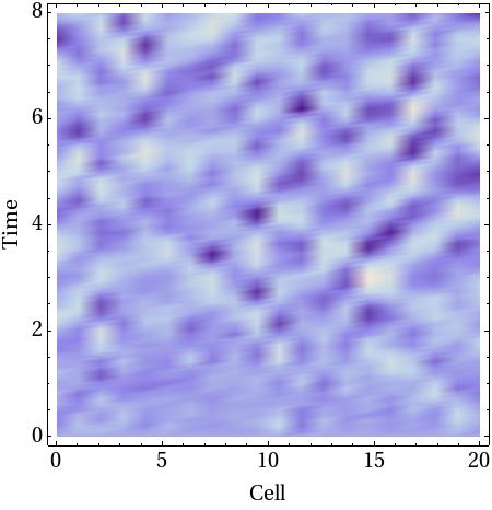
Figure 3: (Color online) Spatio-temporal dynamics of the concentration of $Y$-molecules in the stochastic waves regime. The number of particles, obtained from a single run of the stochastic dynamics, is reported on a scale of shades (with lighter shades indicating a larger number of $Y_{i}$-particles per cell, and dark shades representing low concentrations). Stochastic waves are seen as diagonal structures in the figure, representing both right-moving and left-moving waves. The system considered is a one-dimensional ring of $20$ cells, each of which has a volume $V=5000$. Parameter values are $a=d=\alpha=1$, $\sigma=2$, $c=b=10$ and $\beta=0.1$.

We now turn to the stochastic system and show the spatio-temporal behavior of the concentration of $Y$-molecules in Fig. 3. It is important to stress that we have chosen values of the model parameters such that the deterministic system has a stable homogeneous state. More specifically, for the parameters chosen in Fig. 3, the system is in the stable phase of Fig. 2, but near the line along which a wave instability occurs in the deterministic model. As demonstrated by the diagonal structures in the space-time representation of Fig. 3, the stochastic system displays travelling stochastic waves for this choice of parameters, even if such waves are absent in the deterministic system. In order to illustrate the mechanism producing these stochastic waves we plot the dispersion relations of modes near the wave instability of the deterministic system in Fig. 4 (model parameters other than $c$ are as in the simulations shown in Fig. 3). For $c\gtrsim 9.35$ all modes are stable, and the least stable mode (i.e. the mode for which the real part of the corresponding eigenvalue is maximal among all modes) has an eigenvalue with non-zero imaginary part and negative real part. At $c\approx 9.35$ the wave instability line is crossed, one mode is now marginally stable, and the corresponding eigenvalue is purely imaginary. Crucially, the instability occurs at a non-zero wave number, and with a non-zero imaginary part of the corresponding eigenvalue (see inset). For $c\lesssim 9.35$ the deterministic system has unstable modes and it exhibits travelling waves.

Figure 4: Real part (solid line) and imaginary part (inset, dashed line) of $\lambda(k)$, one of eigenvalues of the Jacobian matrix (19) (the other is its complex conjugate). Model parameters are $a=d=\alpha=1$, $\sigma=2$, $b=10$ and $\beta=0.1$. Using symmetry, we restrict the range of $k$ to a half of the Brillouin zone, $[0,\pi]$. The onset of the travelling wave instability occurs at $c\approx 9.35$.

Figure 5: Upper panel: Temporal evolution of the $Y$-concentration in selected cell in the stochastic waves regime. Data is obtained from one run of the stochastic dynamics, with parameter values as in Fig. 3. Lower panel: Snapshot of the concentration of $Y$-molecules as a function of position at a fixed time $t$.

The stochastic simulations of Fig. 3 are carried out at $c=10$. Here all modes are stable in the deterministic system, the least stable mode has a non-zero wavenumber and a complex eigenvalue. In the absence of intrinsic stochasticity the system would converge to the deterministic homogeneous state. Fluctuations, due to demographic noise at finite cell volumes, however constantly cause random motion about the homogeneous state. At large, but finite cell volumes, a linear approximation is in order and the fluctuations can be decomposed into their Fourier modes. The fluctuations corresponding to the least stable mode decay the slowest, on a time scale set by the real part of the corresponding eigenvalue. This effect, along with fluctuations persistently occurring, conspire due to the mechanism now known as coherent stochastic amplification McKane and Newman (2005). Modes which are stable in the deterministic model can effectively be excited by random fluctuations, and are observed with sizeable amplitude in the stochastic system. In our model this amplitude scales as $V^{-1/2}$ in the cell volume, but the prefactor multiplying this factor can be significant, resulting in stochastic waves with appreciable amplitude even at large cell volumes.

To illustrate the occurrence of stochastic waves further, we show a time-series of the (re-scaled) concentration of Y molecules in a fixed cell in the upper panel of Fig. 5. Coherent stochastic oscillations are clearly visible, their amplitude is seen to scale as $V^{-1/2}$ with the cell volume. Plotting the time series of the Y-concentration in one cell we have effectively disregarded the spatial structure of the system, and focused instead on the temporal dynamics only. In this sense the upper panel of Fig. 5 is similar to observations of amplified stochastic oscillations in the time series of non-spatial systems (see for example McKane and Newman (2005)). The lower panel of Fig. 5 shows the concentration of Y molecules as a function of position at a fixed time. Spatial modulations, again with an amplitude scaling as $V^{-1/2}$, are seen, even though of a lower coherence than the temporal oscillations shown in the upper panel. In this lower panel we have effectively disregarded the temporal dynamics of the system, and have instead focused on its spatial character. The modulations of the concentration of Y molecules as a function of position therefore constitutes the analog of stochastically-driven Turing patterns reported in Butler and Goldenfeld (2009); Biancalani et al. (2010); Scott et al. (2011). The novelty of our model is that it combines the spatial and the temporal aspect; the stochastic waves seen in the nonlocal Brusselator model are noise-driven patterns with structure both as a function of position and as a function of time.

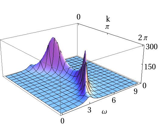
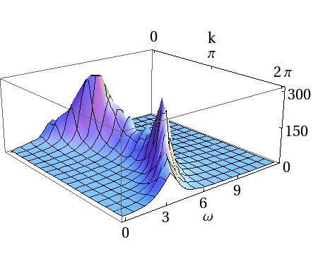
Figure 6: (Color online) Power spectrum of the fluctuations of the $Y$ species obtained analytically (upper panel) from Eq. (III) and numerically (lower panel) by simulating the stochastic process using the Gillespie algorithm. The agreement between the two power spectra is clearly very good. The system is in the stochastic wave regime with $a=d=\alpha=1$, $\sigma=2$, $c=b=10$ and $\beta=0.05$. The spectra show a peaked profile which corresponds to spatio-temporal organization despite the deterministic prediction of a stable homogeneous state. The numerical spectrum is obtained by averaging $200$ realizations of a finite system of $28$ cells each of which has volume $V=1500$.

The theory developed in Sec. III allows us to characterize the observed stochastic waves further. Based on the results of Eqs. (III) we are able to predict the power spectra of spatio-temporal fluctuations about the homogeneous state for any choice of model parameters. Stochastic waves are to be expected whenever the highest peak of these power spectra is found simultaneously at a non-zero wavenumber $k$ (indicating non-trivial spatial structure) and at a non-zero angular frequency $\omega$ (indicating a complex eigenvalue, and hence oscillatory behavior as a function of time). An example of a power spectrum with these properties, obtained from the theory of Sec. III, is shown in the upper panel of Fig. 6; for comparison we show measurements from direct numerical simulations in the lower panel. As seen from this Figure, the agreement between theory and simulations is excellent.

V Conclusion

This paper has been concerned with the investigation of stochastic effects in a nonlocal extension of the Brusselator model. An analysis of this model on the deterministic level reveals that nonlocal interactions can promote the occurrence of travelling wave instabilities, similar to what has been seen before in other chemical reaction models with long-range interactions Nicola et al. (2006). As the main result of our work we show that the nonlocal Brusselator model can also exhibit travelling waves driven by internal fluctuations in parameter regimes in which the deterministic system converges to a homogeneous state. Based on a stochastic formulation of the model in terms of a chemical master equation, and a subsequent expansion in the inverse system size, we derived analytical expressions for the power spectra of these spatio-temporal patterns, in excellent agreement with direct numerical simulations.

These findings extend previous results on noise-driven instabilities. In McKane and Newman (2005) non-spatial systems were considered, and it was shown that intrinsic fluctuations can generate coherent stochastic oscillations for parameters for which the deterministic system spirals into a fixed point. The work of Butler and Goldenfeld (2009); Biancalani et al. (2010); Scott et al. (2011) instead focused on spatial systems, and it was shown that intrinsic noise can generate stochastic Turing patterns, i.e. spatial structures with a constant amplitude in time. Our model combines both aspects, and produces stochastic patterns with a full spatio-temporal dynamics.

These stochastic waves are seen in the power spectra of fluctuations, computed from the theoretical approach, as isolated peaks at non-zero wave number and non-zero angular frequency. While in the past it has been rather difficult to observe spatial stochastic patterns directly, and while most of the previous work was limited to an indirect identification in Fourier space, we have also been able to obtain direct visual confirmation of the stochastic waves in the Brusselator model with nonlocal interaction. Criteria which distinguish stochastic cycles or stochastic patterns from their deterministic analogs (limit cycles and Turing-like patterns) have been proposed Pineda-Krch et al. (2007); Butler and Goldenfeld (2009, 2011). However these are not applicable to systems with nonlocal interactions of the type we have considered here, due to the extra $k$-dependence which comes about because of the nonlocality. It would be interesting to devise criteria which encompass nonlocal models as well.

The purpose of the current work is to illustrate a generic phenomenon which is expected to occur in a wide class of systems; the Brusselator model was chosen to illustrate the basic idea because it is simple and widely studied. The effects of noise on travelling waves has been investigated in the past, but most of these studies depended on the properties of the specific system under consideration. For example, a simple reaction diffusion equation displaying travelling waves is the Fisher equation Fisher (1937). For this system it is known that noise may alter the properties of the waves (see for instance Moro (2001)) and may also be responsible of the emergence of noise-driven travelling waves Hallatschek (2011). However, these waves are different to those we have discussed here, as they do not arise from an underlying unstable homogeneous state. A related point is that the Fisher equation has only one species, whereas we need at least two interacting species, since we require complex eigenvalues to trigger the wave instability Cross and Greenside (2009).

We expect that the mechanism of coherent amplification, applies to more complicated linear instabilities as well Cross and Greenside (2009) and that the concept of stochastic waves is relevant in other models with travelling fronts. We also expect that the analytical formalism we have developed here for spatial systems with nonlocal interaction can successfully be employed to study broader classes of individual-based models. This may include models of the spread of epidemics, in which infection can occur at a distance; deterministic models of such processes have been considered Keeling and Rohani (2008); Wang and Wu (2010). As stochastic patterns are found in more and more model systems, we expect the search for them in real systems to intensify and the understanding of the underlying causes of pattern formation in physical, biological and social systems to broaden.

Appendix A Turing and Wave Instabilities

In this Appendix we derive the conditions which allow the onset of Turing or wave instabilities to be located. Such criteria exist in the literature Turing (1952); Murray (1993); Cross and Greenside (2009), but most of them rely on the standard reaction-diffusion paradigm and will not be applicable in our case which includes a nonlocal kernel, and so an extra $k$-dependence over and above that coming from the diffusion terms. We need therefore a more general approach, described below, which closely follows Nicola (2001).

We start by defining the region of parameter space in which the homogeneous state is stable. Its borders delimitate the instabilities whose type can be determined from the analysis below. The stability condition, $\mbox{Re}[\lambda_{i}(k)]<0$ for all $k$, can be conveniently rewritten using the trace and determinant if the Jacobian is a $2\times 2$ matrix as

$$\mbox{det}\,\mathcal{J}^{*}(k)>0,\quad\mbox{tr}\,\mathcal{J}^{*}(k)<0,\quad\forall k.$$ (33)

The stability region is the set of parameters in which the above inequalities hold. Plotting $\mbox{det}\,\mathcal{J}^{*}(k_{c})$ against $\mbox{tr}\,\mathcal{J}^{*}(k_{c})$ we see that we may leave the stability region by violating one of these inequalities. That is, when

• There exists a $k_{C}\neq 0$ such as $\mbox{det}\,\mathcal{J}^{*}(k_{C})=0$ whereas $\mbox{tr}\,\mathcal{J}^{*}(k)<0\;\forall k$.

• There exists a $k_{C}\neq 0$ such as $\mbox{tr}\,\mathcal{J}^{*}(k_{C})=0$ whereas $\mbox{det}\,\mathcal{J}^{*}(k)>0\;\forall k$.

It is also possible that determinant and trace become simultaneously zero, but this is a degenerate case which we do not consider here.

Now recall that the eigenvalues of the Jacobian are given by

$$\lambda_{1,2}=\frac{1}{2}\left(\mbox{tr}\,\mathcal{J}^{*}\pm\sqrt{\left(\mbox{tr}\,\mathcal{J}^{*}\right)^{2}-4\,\mbox{det}\,\mathcal{J}^{*}}\right),$$ (34)

from which the imaginary part of the eigenvalues may be found. From the discussion at the end of Sec. II we can see that the above conditions defining the boundaries of the stability region correspond respectively to a Turing instability (the former) and to a wave instability (the latter).

The stability conditions as given are not so convenient to deal with directly, because of the presence of inequalities which must be solved for every $k$. To overcome this, we suppose that $\mbox{tr}\,\mathcal{J}^{*}(k)$ has a global maximum at $k_{M}$ and $\mbox{det}\,\mathcal{J}^{*}(k)$ a global minimum at $k_{m}$, a hypothesis that will be discussed further below. In this case the two conditions may be rewritten as:

• (Turing instability) $\mbox{det}\,\mathcal{J}^{*}(k_{m})=0$ and $\mbox{tr}\,\mathcal{J}^{*}(k_{M})<0$.

• (Wave instability) $\mbox{tr}\,\mathcal{J}^{*}(k_{M})=0$ and $\mbox{det}\,\mathcal{J}^{*}(k_{m})>0$.

These are the conditions we have used to obtain Fig. 1 and Fig. 2.

We can now check that the specific forms of $\mbox{tr}\,\mathcal{J}^{*}(k)$ and $\mbox{det}\,\mathcal{J}^{*}(k)$ in our model have the required extrema. Finding the extremal points of $\mbox{tr}\,\mathcal{J}^{*}(k_{M})$ can easily be achieved analytically; for $\mbox{det}\,\mathcal{J}^{*}(k_{m})$ it is a little more difficult. However checking the existence of a global maximum or minimum numerically is straightforward, and we have verified that for the range of parameters of interest to us in this paper such extrema always exist and moreover give the boundaries shown in Fig. 1 and Fig. 2.

Appendix B The van Kampen System-Size Expansion

A description of the general structure and methodology behind the system-size expansion, as applied to the system under consideration, is given in Section III. In this Appendix we give some of the technical details which would otherwise disrupt the flow of the arguments in the main text.

The application of the method is facilitated by writing down the master equation (5) in terms of the step operators (20). An example is given in Eq. (21) for the first reaction of the set of reactions given by Eq. (1). When all eight reactions are included the master equation is given by

$${d\over dt}P_{\textbf{n},\textbf{m}}(t)=$$ (35)

$$= \sum_{i=-\infty}^{\infty}\Biggl{[}(\epsilon_{X,i}^{-}-1)\;T(n_{i}+1,m_{i}|n_{i},m_{i})$$

$$+(\epsilon_{X,i}^{+}-1)\;T(n_{i}-1,m_{i},|n_{i},m_{i})$$

$$+(\epsilon_{X,i}^{+}\>\epsilon_{Y,i}^{-}-1)\;T(n_{i}-1,m_{i}+1|n_{i},m_{i})$$

$$+(\epsilon_{X,i}^{-}\>\epsilon_{Y,i}^{+}-1)\;T(n_{i}+1,m_{i}-1|n_{i},m_{i})$$

$$+\sum_{j\in\{i-1,i+1\}}\biggl{(}(\epsilon_{X,i}^{+}\>\epsilon_{X,j}^{-}-1)\;T(n_{i}-1,n_{j}+1|n_{i},n_{j})$$

$$+(\epsilon_{X,j}^{+}\>\epsilon_{X,i}^{-}-1)\;T(n_{i}+1,n_{j}-1|n_{i},n_{j})$$

$$+(\epsilon_{Y,j}^{+}\>\epsilon_{Y,i}^{-}-1)\;T(m_{i}+1,m_{j}-1|m_{i},m_{j})$$

$$+(\epsilon_{Y,i}^{+}\>\epsilon_{Y,j}^{-}-1)\;T(m_{i}-1,m_{j}+1|m_{i},m_{j})\biggr{)}\Biggr{]}$$

$$\times P_{\textbf{n},\textbf{m}}(t).$$

The fundamental ansatz of the system-size expansion is given by Eq. (22) in the main text. It leads to the expression (24) for the left-hand side of the master equation. The right-hand side can be evaluated by observing that the step operators (20) can be expanded in the inverse of the square root of the system size, $V^{-\frac{1}{2}}$, giving rise to the following expressions van Kampen (2007):

$$\epsilon_{X,i}^{\pm}\approx 1\pm\frac{1}{\sqrt{V}}\partial_{\xi_{i}}+\frac{1}{2V}\partial^{2}_{\xi_{i}},\quad\epsilon_{Y,i}^{\pm}\approx 1\pm\frac{1}{\sqrt{V}}\partial_{\eta_{i}}+\frac{1}{2V}\partial^{2}_{\eta_{i}}.$$ (36)

This together with the substitution of the ansatz (22) into the transition rates (2), and the replacement of $P_{\mathbf{n},\mathbf{m}}(t)$ by $\Pi(\bm{\xi},\bm{\eta},t)$, allows us to expand the right-hand side in powers of $V^{-\frac{1}{2}}$.

Equating the left- and right-hand sides of the master equation gives the general form

$$\begin{split}&\partial_{t}\Pi-\sqrt{V}\>\nabla_{\bm{\xi}}\Pi\cdot\partial_{t}\bm{\phi}-\sqrt{V}\>\nabla_{\bm{\eta}}\Pi\cdot\partial_{t}\bm{\psi}\\ &=\left\{-\frac{1}{\sqrt{V}}\left[\bm{f}(\bm{\phi},\bm{\psi})\cdot\nabla_{\bm{\xi}}+\bm{g}(\bm{\phi},\bm{\psi})\cdot\nabla_{\bm{\eta}}\right]+\frac{\mathbf{L}}{V}\right\}\Pi,\end{split}$$ (37)

where $\mathbf{L}$ is a linear operator containing various derivatives in $\eta$ and $\xi$ and $\bm{f}$ and $\bm{g}$ are functions of $\bm{\phi}$ and $\bm{\psi}$. After the introduction of a re-scaled time $\tau=t/V$, Eq. (25) of the main text is obtained. This is now in a form where the various terms on both sides of the equation can be balanced.

Equating the leading order terms in Eq. (25) gives equations whose general structure is displayed in Eq. (26) and whose specific form in Eq. (II). Equating the next-to-leading order terms gives an equation with general structure (27) and specific form

$$\partial_{\tau}\Pi = \sum_{i=-\infty}^{\infty}\left(-\sum_{r=1}^{2}\partial_{\zeta_{r,i}}\left(\mathcal{A}_{r,i}\Pi\right)\right.$$ (38)

$$\left.+\frac{1}{2}\sum_{r,s=1}^{2}\sum_{j=i-1}^{i+1}\partial_{\zeta_{s,i}}\partial_{\zeta_{r,j}}\left[\mathcal{B}_{rs,ij}\Pi\right]\right),$$

where for convenience we have introduced the notation $\zeta_{1}\equiv\xi$ and $\zeta_{2}\equiv\eta$. The precise forms of $\mathcal{A}_{r,i}$ and of $\mathcal{B}_{rs,ij}$ will be discussed below, but as mentioned in the main text it is easier for our purposes to work with the equivalent Langevin equation Gardiner (2009); Risken (1989)

$$\frac{d\bm{\zeta}_{i}}{d\tau}=\mathcal{A}_{i}(\bm{\zeta})+\bm{\mu}_{i}(\tau),$$ (39)

where $\bm{\mu_{i}}$ is a Gaussian noise with zero mean and correlator

$$\langle\bm{\mu}_{i}(\tau)\bm{\mu}_{j}^{\rm T}(\tau^{\prime})\rangle=\mathcal{B}_{ij}\,\delta(\tau-\tau^{\prime}).$$ (40)

We are then able to take the Fourier transform of this equation in both space and time to give Eq. (28).

The Langevin equation (28) is defined by two matricies: the drift matrix and the diffusion matrix. Since the drift matrix is identical to the Jacobian of the system, as presented in Eq. (30), we will only give the expression for the diffusion matrix.

The diffusion matrix $\mathcal{B}$ has elements $\mathcal{B}_{rs,ij}$ where $r$ and $s$ index the species and $i$ and $j$ the cell. In the following the expressions are given for each $r$ and $s$ and for a given cell $i$. The only non-zero values of $\mathcal{B}_{rs,ij}$ occur when $j=i-1,i$ or $i+1$, and these are given respectively as the first, second and third entries of a row vector:

$${\mathcal{B}}_{11,i}=\Biggl{(}-\alpha\Bigl{(}\phi_{i}+\phi_{i-1}\Bigr{)},\quad a+(b+d)\>\phi_{i}$$

$$+c\>\Lambda\sum_{j=-\infty}^{\infty}e^{-\sigma|j|}\>\phi_{i}^{2}\psi_{i-j}+\alpha\Bigl{(}\phi_{i-1}+2\phi_{i}+\phi_{i+1}\Bigr{)},$$

$$\quad-\alpha\Bigl{(}\phi_{i}+\phi_{i+1}\Bigr{)}\Biggr{)},$$

$${\mathcal{B}}_{12,i}={\mathcal{B}}_{21,i}=$$

$$=\Biggl{(}0,\quad-b\phi_{i}-c\>\Lambda\sum_{j=-\infty}^{\infty}e^{-\sigma|j|}\>\phi_{i}^{2}\psi_{i-j},\quad 0\Biggr{)},$$

$${\mathcal{B}}_{22,i}=\Biggl{(}-\beta\Bigl{(}\psi_{i}+\psi_{i-1}\Bigr{)},\quad b\>\phi_{i}$$

$$+c\>\Lambda\sum_{j=-\infty}^{\infty}e^{-\sigma|j|}\>\phi_{i}^{2}\psi_{i-j}+\beta\Bigl{(}\psi_{i-1}+2\psi_{i}+\psi_{i+1}\Bigr{)},$$

$$\quad-\;\beta\Bigl{(}\psi_{i}+\psi_{i+1}\Bigr{)}\Biggr{)}.$$

Evaluating them in the homogeneous state gives

$$\begin{split}{\mathcal{B}}^{*}_{11,i}&=\left[\begin{array}[]{r}-\dfrac{2a\alpha}{d},\quad 2a+\dfrac{2ab}{d}+\dfrac{4a\alpha}{d},\quad-\dfrac{2a\alpha}{d}\end{array}\right],\\ {\mathcal{B}}^{*}_{12,i}&={\mathcal{B}}^{*}_{21,i}=\left[\begin{array}[]{r}0,\quad-\dfrac{2ab}{d},\quad 0\end{array}\right],\\ {\mathcal{B}}^{*}_{22,i}&=\left[\begin{array}[]{r}-\dfrac{2bd\beta}{ac},\quad\dfrac{2ab}{d}+\dfrac{4bd\beta}{ac},\quad-\dfrac{2bd\beta}{ac}\end{array}\right].\end{split}$$ (42)

The structure of ${\cal B}_{rs,ij}^{*}$ can be seen from Eq. (42) to be

$${\cal B}^{*}_{rs,ij}=b^{(0)}_{rs}\delta_{i-j,0}+b^{(1)}_{rs}\delta_{|i-j|,1},$$ (43)

where the two matrices $b^{(0)}$ and $b^{(1)}$ can be read off from Eq. (42). It is then straightforward Lugo and McKane (2008) to calculate the spatial Fourier transform, $\tilde{\cal B}_{rs}\equiv\tilde{\cal B}_{rs}(k)$, of the matrices (42) with respect to the variable $i-j$:

$$\tilde{\cal B}_{rs}^{*}(k)=(b^{(0)}_{rs}+2b^{(1)}_{rs})+b^{(1)}_{rs}\tilde{\Delta},$$ (44)

where $\tilde{\Delta}$ is given by Eq. (17). The explicit forms are

$$\tilde{\cal B}_{11}^{*}(k) = \frac{2a}{d}\left(b+d\right)-\frac{2a\alpha}{d}\tilde{\Delta},$$

$$\tilde{\cal B}_{12}^{*}(k) = \tilde{\cal B}_{21}^{*}(k)=-\frac{2ab}{d},$$

$$\tilde{\cal B}_{22}^{*}(k) = \frac{2ab}{d}-\frac{2bd\beta}{ac}\tilde{\Delta}.$$ (45)

The power spectra of the stochastic oscillations, defined by Eq. (31), have the form (III). The functions ${\cal C}_{X}$ and ${\cal C}_{Y}$ are defined by

$${\cal C}_{X}(k) = \tilde{\cal B}_{11}^{*}(k)\>{\cal J}_{22}^{*}(k)^{2}-2\>\tilde{\cal B}_{12}^{*}(k)\>{\cal J}_{12}^{*}(k)\>{\cal J}_{22}^{*}(k)$$

$$+\tilde{\cal B}_{22}^{*}(k)\>{\cal J}_{12}^{*}(k)^{2},$$

$${\cal C}_{Y}(k) = \tilde{\cal B}_{22}^{*}(k)\>{\cal J}_{11}^{*}(k)^{2}-2\>\tilde{\cal B}_{12}^{*}(k)\>{\cal J}_{21}^{*}(k)\>{\cal J}_{11}^{*}(k)$$ (46)

$$+\tilde{\cal B}_{11}^{*}(k)\>{\cal J}_{21}^{*}(k)^{2}.$$