Infrared-Faint Radio Sources: A Cosmological View

Abstract

Context. Infrared Faint Radio Sources (IFRS) are extragalactic emitters clearly detected at radio wavelengths but barely detected or undetected at optical and infrared wavelengths, with 5$\sigma$ sensitivities as low as 1 $\mu$Jy.

Aims. Recent SED-modelling and analysis of their radio properties shows that IFRS are consistent with a population of (potentially extremely obscured) high-redshift AGN at 3 $\leq$ z $\leq$ 6. We demonstrate some astrophysical implications of this population and compare them to predictions from models of galaxy evolution and structure formation.

Methods. We compiled a list of IFRS from four deep extragalactic surveys and extrapolated the IFRS number density to a survey-independent value of (30.8$\pm$15.0) deg^-2. We computed the IFRS contribution to the total number of AGN in the Universe to account for the Cosmic X-ray Background. By estimating the black hole mass contained in IFRS, we present conclusions for the SMBH mass density in the early universe and compare it to relevant simulations of structure formation after the Big Bang.

Results. The number density of AGN derived from the IFRS density was found to be $\sim$ 310 deg^-2, which is equivalent to a SMBH mass density of the order of $10^{3}$ M_☉ Mpc^-3 in the redshift range 3 $\leq$ z $\leq$ 6. This produces an X-ray flux of $9\cdot 10^{-16}$ W m^-2 deg^-2 in the 0.5-2.0 keV band and $3\cdot 10^{-15}$ W m^-2 deg^-2 in the 2.0-10 keV band, in agreement with the missing unresolved components of the Cosmic X-ray Background. Concerning the problem of SMBH formation after the Big Bang we find evidence for a scenario involving both halo gas accretion and major mergers.

1 Introduction

Infrared-Faint Radio Sources (IFRS) were first classified by Norris et al. (2006), who identified them as sources detected at 1.4 GHz using the the Australia Telescope Compact Array (ATCA), but absent in deep infrared images from the Spitzer Wide-Area Infrared Extragalactic (SWIRE) survey (Lonsdale et al. 2003). In the process of matching IR counterparts to radio sources from the Australia Telescope Large Area Survey (ATLAS), Norris et al. found a total of 22 radio sources to which no infrared counterpart could be reasonably identified in any of the observed Spitzer bands (3.6 $\mu$m – 24 $\mu$m), down to a sensitivity of $\sigma_{3.6\,\mu m}\,=\,1.0\,\mu$Jy. A similar result was obtained by Middelberg et al. (2008a) who found 31 IFRS in the ELAIS-S1 at similar IR and radio sensitivities. A substantial fraction of these IFRS have flux densities of several mJy at 1.4 GHz, and some are even found at 20 mJy.

A first attempt to investigate the nature of the IFRS discovered in the ATLAS survey was undertaken by Norris et al. (2007), who observed two IFRS with Very Long Baseline Interferometry (VLBI), and detected one. They argued that IFRS are AGN-driven objects because the VLBI detection indicated a brightness temperatures in excess of $10^{6}$ K. Such high temperatures cannot be reached by thermal emission mechanisms and hence indicate non-thermal radio emission produced by an AGN. Later Middelberg et al. (2008b), also using VLBI observations, confirmed that at least a fraction of the IFRS population must contain an AGN contributing to the total IFRS spectral energy distribution.

These results were complemented by Garn & Alexander (2008) who identified an IFRS population in the Spitzer extragalactic First Look Survey (xFLS). Modelling their spectral energy distributions (SEDs) with template SEDs from known objects to estimate IFRS redshifts, they found that the characteristics of IFRS resembled a variety of 3C sources redshifted to 2 $\leq$ z $\leq$ 5. A more detailed SED analysis was presented by Huynh et al. (2010), who used new, very deep Spitzer data in the Chandra Deep Field South (CDF-S) field obtained during two Spitzer legacy programs, SIMPLE (Damen et al., in prep.) and FIDEL (PI: Dickinson). With a sensitivity of $\sigma_{3.6\,\rm{\mu m}}\,=\,0.16\,\mu$Jy, IR counterparts for two of the four investigated IFRS were identified. Furthermore, a faint optical counterpart (V = 26.27 AB-mag) to one of the IFRS was serendipitously identified within the GOODS HST/ACS imaging campaign (Giavalisco et al. 2004). A second IFRS located within the GOODS-South field was found to have no optical detection at all (implying V $>$ 28.9 AB-mag), putting strong constraints on their SEDs. Huynh et al. also searched other deep multi-wavelengths data sets in the CDF-S for counterparts, in particular the Chandra 2 Ms source catalog (Luo et al. 2008), the GEMS HST imaging campaign (Rix et al. 2004) and the MUSYC catalog (Gawiser et al. 2006). These searches did not yield any counterparts in the X-ray or the optical/NIR regime. Modelling template SEDs to represent the radio and, if available, the IR and optical detections, Huynh et al. (2010) found that a 3C 273-like object can reproduce the data when redshifted to z = 2 (IR-detection) and z $>$ 4 (IR non-detection). The IR non-detections could not be explained by any template SED at redshifts smaller than $\sim$4. These estimates constrain the redshift range of IFRS, placing at least a significant fraction of them at z $>$ 4. On the other hand, given that none of the IFRS was detected at 24 $\mu$m, Huynh et al. (2010) conclude that IFRS fall well beyond the IR-radio correlation (see e.g. Appleton et al. 2004, whose $q_{24}\,=\,\log\left(S_{24\,\rm{\mu m}}/S_{20\,\rm{cm}}\right)$ parameter of 0.84 would imply a 24 $\mu$m flux density of 7 mJy for a typical IFRS with S${}_{20\,\rm{cm}}\,=\,1\,$mJy). Hence the IFRS radio emission can not be explained by star-forming processes but is likely to be produced by AGN. This finding is supported by applying various calibrations of the 1.4 GHz luminosity as star formation rate (SFR) tracer. For instance, the classical calibration by Bell (2003) gives star formation rates of around a million solar masses per year for a typical IFRS assumed to be located at z = 4, which is unphysical and hence suggests that the radio emission of IFRS cannot be only caused by star formation.

Using new radio data spanning 2.3 GHz to 8.6 GHz, Middelberg et al. (2011) analysed the radio properties of 18 ATLAS IFRS. They found unusually steep radio spectral indices with a median $\alpha$ of $-1.4$ ($S\propto\nu^{\alpha}$), and no spectral index flatter than $-0.5$. According to the z–$\alpha$ relation (e.g. Athreya & Kapahi 1998) that predicts steeper radio spectral indices at higher redshifts, these findings suggest that IFRS reside in the high-redshift Universe. Another result from Middelberg et al. is that the ratio between radio and IR flux densities, $S_{20\,\rm{cm}}/S_{3.6\,\rm{\mu m}}$, is much larger for IFRS than for the general radio source population, and potentially exceeds $10^{4}$, a value which is similar to that found in a sample of high redshift radio galaxies (HzRGs) by Seymour et al. (2007). These ratios and redshift dependencies are further investigated in more detail by Norris et al. (2011). They suggest that IFRS have redshifts of z $\sim$ 5 in the most extreme cases, because no 3.6 $\mu$m counterpart could be identified by stacking ultra-deep Spitzer observations at the location of 39 IFRS, reaching a stacked sensitivity of $S_{\rm 3.6\,\mu m}\sim$0.2 $\mu$Jy.

In summary, the evidence from SED modelling, very high $S_{20\,\rm{cm}}/S_{3.6\,\rm{\mu m}}$ ratios and steep spectral indices all suggest that IFRS are at high redshifts (at least z $>$ 2) and contain AGN. In this paper we present the implications of this population for the AGN number densities, the Cosmic X-ray background (CXB), and structure formation models. Throughout this paper, we adopt a standard flat $\Lambda$CDM cosmology with $H_{0}\,=\,71$ km s^-1 Mpc^-1 and $\Omega_{M}$ = 0.27.

2 Catalogue of known IFRS

In previous publications the selection criterion used to identify IFRS was simply “radio sources with no apparent IR counterpart”. This is a rather loose definition, and we propose to replace this definition by the following two criteria:

• The ratio of radio to mid-IR flux, $S_{20\,\rm{cm}}/S_{3.6\,\rm{\mu m}}$, exceeds 500.

• The 3.6 $\mu$m flux density is smaller than 30 $\mu$Jy.

The first criterion selects objects with extreme radio to IR flux ratios, making IFRS clear outliers from the IR-radio correlation. This encapsulates the requirement that IFRS are strong in the radio, but weak at infrared wavelengths. The second criterion ensures that the sources are at significant, cosmologically relevant, distances, to eliminate low-redshift radio-loud AGNs. For example, Cygnus A (with $S_{20\,\rm{cm}}/S_{3.6\,\rm{\mu m}}$ $=$ 2$\cdot$10⁵) would be an IFRS based on its radio to IR flux ratio alone, but would be excluded by the 3.6 $\mu$m flux density cutoff.

Alonso-Herrero et al. (2006) have shown that the near-to-mid-IR SEDs of galaxies dominated by AGN emission exhibit a power-law behaviour produced by re-emission from warm dust surrounding the AGN. They find that AGN can span a large range of optical-to-IR spectral slopes with a maximum $\alpha=-2.8$ but typically between $-0.5$ and $-1.0$. These values are similar to those observed in the radio. In fact, the k-corrections necessary to estimate the intrinsic $S_{20\,\rm{cm}}/S_{3.6\,\rm{\mu m}}$ values would produce a small difference with respect to the observed ones. It is evident that the first criterion preferably select IFRS if the spectral slope in the near-IR is steeper than in radio, i.e. star-forming galaxies (with flatter spectra due to a dominant stellar emission) are preferrably scattered away from the sample. This weak dependency for $S_{20\,\rm{cm}}/S_{3.6\,\rm{\mu m}}$ as a function of redshift suggests that IFRS are intrinsically extreme outliers of the IR-radio correlation. This leaves the second criterion as the dominant to preferentially select high-redshift sources using the dimming produced by cosmic distance.

Applying our criteria, we present in this paper a catalogue containing all IFRS found in the ATLAS/CDF-S (Norris et al. 2006) and ATLAS/ELAIS-S1 (Middelberg et al. 2008a) surveys, in the Spitzer extragalactic First Look Survey (xFLS, Condon et al. 2003), and in the COSMOS survey (Schinnerer et al. 2007). To date, this compilation is the most comprehensive list of IFRS, including 55 objects located in four individual surveys. The surveys were chosen not only because of their radio and IR coverage but also for the covered area. To minimise the effects of cosmic variance, only surveys greater than 1 deg² were analysed. Cosmic variance can be a significant source of error when measuring density-related quantities especially in small survey fields. For example, the GOODS field was analysed for cosmic variance by Somerville et al. (2004). They found that for fields in the order of several 100 arcmin², such as GOODS, the error of number density estimates can range from 20% up to 60% for strongly clustered sources. To avoid statistical errors introduced by cosmic variance in the estimated number counts, we have excluded small area surveys. In particular we have left out the deep surveys in the Lockman Hole East (Ibar et al. 2009) and Lockman Hole North (Owen & Morrison 2008). An overview of the surveys we used is shown in Table 1.

Table 1: Summary of investigated surveys.

Survey	Area	3.6 $\mu$m limit	20 cm limit	IFRS
Name	deg2	$\mu$Jy	$\mu$Jy	number
ATLAS/CDF-S	3.7	3.1	186	14
ATLAS/ELAIS-S1	3.6	3.1	160	15
First Look Survey	3.1	9.0	105	13
COSMOS	1.1	1.0	65	13

The source selection process was as follows: a pre-selection of candidate sources was obtained by cross-matching radio and IR catalogues of each survey in two different ways. Clearly extended radio sources, or those consisting of multiple components, were excluded from this pre-selection to prevent resolved AGN lobes entering the sample. All radio sources with a 3.6 $\mu$m counterpart within a 5$\arcsec$ radius were selected and their $S_{20\,\rm{cm}}/S_{3.6\,\rm{\mu m}}$ ratio was calculated. For all radio sources that did not have a 3.6 $\mu$m counterpart within 5″, the 5$\sigma$ detection limit of each survey as listed in Table 1 was chosen to provide a conservative upper limit on the 3.6 $\mu$m flux density. Hence the inferred $S_{20\,\rm{cm}}/S_{3.6\,\rm{\mu m}}$ is a lower limit, and is indicated as such in Table 2. A 5$\arcsec$ search radius for cross-matching the radio and 3.6 $\mu$m data ensures that at any redshift greater than z = 0.5, the corresponding linear distance is on the order of 30 kpc or more, and so exceeds the size of a large spiral galaxy. We then produced postage stamp images for visual inspection of each candidate source, showing a grey-scale IR image centred on the radio position of the source with overlaid radio contours. These images were inspected by eye to determine whether the source really is an IFRS or whether the cross-matching process failed, e.g. because of an uncatalogued IR counterpart. We also addressed the problem of source blending due to the different resolutions of the IR and radio images (FWHM of 1.66$\arcsec$ in the IRAC $3.6\,\rm{\mu m}$ channel, Fazio et al. 2004, vs. 11$\arcsec$ by 5$\arcsec$ in the ATLAS 1.4 GHz radio data). IFRS candidates with more than one plausible IR counterpart were rejected in the selection process, since $S_{20\,\rm{cm}}/S_{3.6\,\rm{\mu m}}$ could not be reliably determined. The final sample of 55 sources is listed in Table 2, and a histogram showing the distribution of radio SNR is shown in Figure 1.

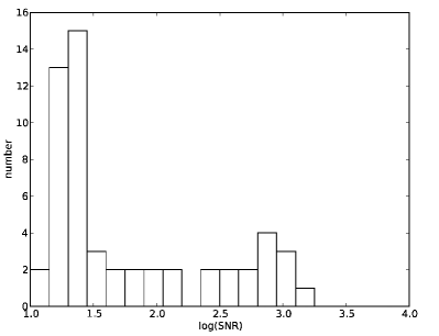
Figure 1: Histogram of the SNR distribution at 20 cm for all IFRS presented in this paper. Note that the abscissa is logarithmic.

Note that the visual inspection of candidate sources helped to keep the rate of false detections (i.e., arising from imaging artefacts) to a minimum. The survey sensitivities in Table 1 were obtained by calculating the median of the rms at the source positions, as provided in the respective catalogues. We used this as characteristic survey sensitivity rather than adopting the sensitivity limits given in the relevant publications because those limits were often related to the most sensitive regions of the observed areas, and thus were not representative.

3 IFRS Densities

3.1 The sample

To derive an estimate of IFRS surface density, at least to within an order of magnitude, we analysed the four surveys quoted above. We used surveys with different sensitivities to extrapolate to the total surface density of IFRS in the Universe.

As shown in Table 1, the surface density of IFRS strongly depends on the sensitivity of the individual radio surveys, whereas the IR sensitivity seems to have little effect. The errors for the individual measurements were obtained as follows: the error in radio sensitivity is the Median Absolute Deviation (MAD) of the rms values at the position of the targets from a given radio survey. This measure is robust against outliers and can characterise non-Gaussian distributions. Assigning errors to the measured IFRS surface densities is more complicated. We chose to follow a statistical ansatz claiming that there is an intrinsic IFRS surface density at the sensitivity limit of a given survey, $\lambda_{intr}$, and the IFRS surface density that we actually measured for that survey, $\lambda_{meas}$. Assuming a Poissonian distribution (because the IFRS surface density is always greater than zero and discrete), we determined the 95 % confidence levels with which one would measure a surface density of $\lambda_{meas}$, given the true surface density is $\lambda_{intr}$. Because the Poisson distribution is asymmetric, this procedure yielded asymmetric errors for the surface densities.

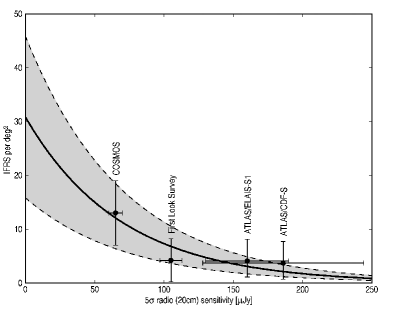
Figure 2: Plot illustrating the extrapolation of IFRS surface density with respect to different radio sensitivities. The best fit (solid line) is given by $\lambda\,=\,(30.8\pm 15.0)\exp\{(-0.014\pm 0.006)5\sigma_{radio}\}$, its quality in terms of $\chi^{2}/d.o.f.$ is 5.5, Pearson’s correlation coefficient is $R^{2}\,=\,0.82$. The dashed curves that limit the shaded area correspond to fit functions representing the minimum and maximum values for the IFRS surface density with respect to the error or $\pm$ 15.0 given above.

To extrapolate the measured densities to an intrinsic IFRS surface density (what a radio observation with zero noise would yield), an exponential fit was used to model the measurements (shown in Fig. 2). We chose an exponential function because of a theoretical and a practical reason. The theoretical reason is that the function should be monotonic because there is no obvious reason why the IFRS surface density should peak around a certain sensitivity. The practical reason is that in our tests an exponential function yielded the best results with respect to a $\chi^{2}$ test ($\chi^{2}/d.o.f.$ = 5.5). We thus define the extrapolated IFRS surface density as the value given by the y-axis intersect of the fit at $(30.8\pm 15.0)$ IFRS/deg². We point out that this large error is real, underlining the fact that this calculation has to be understood as “order of magnitude” estimate only.

3.2 Motivation of a redshift range for IFRS

To convert the surface density of IFRS to a space density we assume that the bulk of IFRS populate the redshift range 3 $\leq$ z $\leq$ 6. There are several motivations for this choice: (i) it has been suggested by the SED modelling work described in Section 1 that most IFRS SEDs are inconsistent with template SEDs displaced to redshifts significantly less than z = 4; (ii) those few IFRS detected in 3.6$\mu$m with this ultra-deep IR data are at least at z = 2 (conclusions in Huynh et al. 2010); (iii) the radio to IR flux density ratios of IFRS are similar to that of the Seymour et al. (2007) HzRG sample, of which many sources have redshifts of 3 and above; (iv) IFRS have very steep radio spectra, which indicate high redshifts according to the z–$\alpha$ relation. However, since there is a large intrinsic scatter in the z–$\alpha$ relation as e.g. given by Athreya & Kapahi (1998), we do not give quantitative redshift estimates based on this relation but only employ it as a qualitative hint. Therefore we adopt z = 3 to be a good compromise as lower limit for their redshift range.

The upper limit of z = 6 was chosen because of the scarcity of sources beyond this redshift, as has been found, e.g., in the Sloan Digital Sky Survey (SDSS; see e.g. Schneider et al. 2010; Fan et al. 2003). Whilst there is a significant number of quasars at redshifts of z $\sim$ 5, their number rapidly decreases beyond z $\sim$ 6, with only very few spectroscopically confirmed quasars having redshifts significantly greater than 6. Hence z = 6 is a reasonable upper limit for our estimates. The problem of obtaining redshift estimates for IFRS is discussed in more detail by Norris et al. (2011), who argue for redshifts as high as z = 5, using extrapolations of the $S_{20\,\rm{cm}}/S_{3.6\,\rm{\mu m}}$ ratios and 3.6 $\mu$m flux densities of typical IFRS.

Furthermore, to also get a theoretically motivated estimate of the minimum redshift for a typical IFRS, we extended the work by Huynh et al. (2010) who modelled the SEDs of IFRS by known template SEDs of different astrophysical objects (see Sec. 1). We chose 3C 48 with an intrinsic redshift of 0.37 as template. 3C 48 is an excellent candidate for being an IFRS at higher redshifts because of its intrinsic high $S_{20\,\rm{cm}}/S_{3.6\,\rm{\mu m}}$ ratio; it therefore does not require huge amounts of obscuring dust to dim down the observed NIR. We redshifted it to z = 5, boosted it in flux by a constant factor of 5 and dimmed it in the optical in NIR wavelength range using a Calzetti et al. (2000) reddening law with $A_{V}\,=\,1$. The resulting model SED can reproduce all observational characteristics of a typical IFRS. This result is illustrated in Fig. 3.

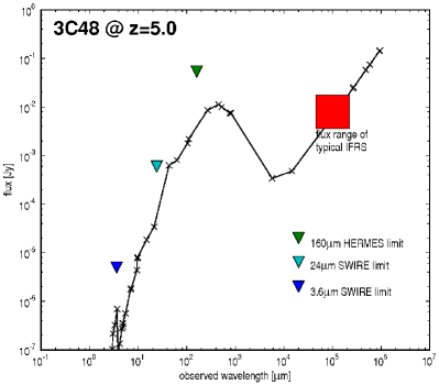
Figure 3: The template SED of 3C 48, redshifted to z = 5, boosted in flux by a wavelength-independent factor of 5 and dimmed in the optical and NIR following a Calzetti et al. (2000) extinction law with $A_{V}\,=\,1$. To emphasise that this SED is the one of an IFRS, we give the detection limits of the SWIRE survey described in sect. 1 as well as the 160 $\mu$m limit of the planned Herschel Hermes survey. The radio spectral index of this SED corresponds to $\alpha\,=\,-1.4$.

Using this model SED, we traced the evolution of its $S_{20\,\rm{cm}}/S_{3.6\,\rm{\mu m}}$ flux ratio as a function of redshift. We also included several radio spectral indices in our calculations to account for different radio components (e.g. bremsstrahlung, aged synchrotron or flat AGN spectra) which could yield different radio spectral indices than the canonical $\alpha\,=\,-0.7$ ($S_{\nu}\propto\nu^{\alpha}$) for thermal synchrotron emission. Thus we account for the radio spectral indices being typically lower towards higher redshift.

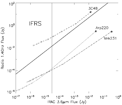
Figure 4: Tracks showing the evolution of the radio and NIR luminosity of a 3C 48-like model with redshift. The redshift data points are given from right to left, starting with 3C 48’s (and the other two comparative sources, Mrk 231 and Arp 220) intrinsic redshift (bold open square). The first thin open square from right indicates a redshift of z = 1, the next thin open square is equal to z = 2 and so on to z = 7. The vertical solid line indicates the IFRS NIR flux cutoff-criterion $S_{3.6\,\rm{\mu m}}\,<\,30\,\mu$Jy, the other solid line represents $S_{20\,\rm{cm}}/S_{3.6\,\rm{\mu m}}\,=\,500$.

The resulting plot (Fig. 4) shows that only beyond a redshift of $z=3$ 3C 48-like models are able to reproduce the high $S_{20\,\rm{cm}}/S_{3.6\,\rm{\mu m}}$ flux ratios and the low 3.6 $\mu$m flux densities observed in IFRS. Our model calculations indicate that to reproduce the observed 1.4 GHz flux densities of a few mJy, steep spectral indices are preferred, which is in agreement with the results obtained by Middelberg et al. (2011).

3.3 The space density of IFRS and their SMBH

In our redshift range of $z=3-6$, a solid angle of 1 deg² corresponds to a comoving volume of $21.5\cdot 10^{6}$ Mpc³ (Wright 2006), and so the observed surface density of IFRS converts to an IFRS space density simply by dividing the extrapolated number density of IFRS per deg² by the comoving volume:

$$n_{IFRS}\,=\,1.44\cdot 10^{-6}\,\rm{Mpc}^{-3}$$ (1)

This space density can now be converted into a mass density of Supermassive Black Holes (SMBHs) that power IFRS. However, simply adopting SMBH masses found in recent studies of large quasar surveys as described in Vestergaard et al. (2008) for the SDSS data release 3 (containing more than 15 000 quasars up to z = 5) would lead to an overestimation of SMBH masses because the limits of contemporary optical surveys prevent from detecting high-z quasars with less than $M_{SMBH}\,\sim\,10^{8}\,$M_☉. The actual limit for the SDSS is about $3\cdot 10^{8}\,$M_☉ and is based on the line width of broad emission lines in a quasar spectra to determine $M_{SMBH}$ from their equivalent width. When converted to optical luminosities, this corresponds to a lower limit of $M_{i}\,=\,-27.5$ for a z = 4 quasar. IFRS cannot be optically bright quasars, because this would require large amounts of dust in their surrounding in order to maintain their IFRS nature, hence one has to lower the average SMBH mass found by Vestergaard et al. (2008); Vestergaard & Osmer (2009) for high-redshift AGN of $\langle M_{SMBH}\rangle\,\sim\,10^{9}\,$M_☉ (this value is supported by other work with much smaller quasar samples but more accurate methods for determining $M_{SMBH}$, see e.g. Dietrich & Hamann 2004; Fine et al. 2008). For example, an SMBH radiating at its Eddington limit produces an unobscured z = 4 quasar with an apparent magnitude of 25.0 (a common limit for contemporary optical surveys carried out with space-based facilities) while having a mass of only $3.5\cdot 10^{6}\,$M_☉. Recent cosmological hydrodynamical simulations (e.g. Degraf et al. 2010) showed that most SMBHs at z = 5 do not accrete at their Eddington limit but at a factor of approximately 5 to 10 times less. Nevertheless, observational evidence for the $L_{Bol}/L_{Edd}$ ratio indicates an accretion mechanism at $L_{Bol}/L_{Edd}\,=\,1$ for the most distant quasars (Fan 2009). This discrepancy between theory and observations could be a selection effect in currently available observations because SMBHs not accreting at their Eddington limit would simply be too faint to be detected. Therefore we conclude that optical observations are unsuitable to estimate a typical SMBH mass for IFRS.

Another way to estimate the SMBH masses in IFRS are X-ray observations which are thought to be an efficient way to detect large numbers of AGN. X-rays can leave the emission regions rather unabsorbed, and there is little contamination from other sources, such as stars. Given that no IFRS identified in the radio observations of the ELAIS-S1 field is detected in the corresponding X-ray survey by Puccetti et al. (2006), we can use this information to derive an upper limit for a SMBH. Using Equation 5, a $4\cdot 10^{7}\,{\rm M}_{\sun}$ SMBH at z = 4.5 would just not be visible in the 0.5-2.0 keV band, given the detection limits of the Puccetti et al. (2006) survey of 5.5$\cdot$10^-19 W m^-2. Unfortunately, no IFRS is located in the CDF-S Chandra 2 Ms observation by Luo et al. (2008). The X-ray observations done within the COSMOS survey using XMM-Newton (Cappelluti et al. 2007, best sensitivity of 7.2$\cdot$10^-19 W m^-2 in the soft band) did not yield a clear identification of an IFRS X-ray counterpart, too. We note that especially for the inner parts of the COSMOS X-ray image, the field is very crowded which makes the reliable detection of potentially very weak counterparts difficult. However, to provide some margin (to account for extinction, for example), we approximately double this value and therefore assume an upper limit for the mass for SMBHs in IFRS of $M_{IFRS}\,\leq\,10^{8}\,$M_☉. Hence the mass density of SMBH in IFRS is:

$$\rho_{IFRS}\,\leq\,1.4\cdot 10^{2}\,\rm{M_{\sun}\,Mpc}^{-3}$$ (2)

4 Implications

4.1 … on AGN Source Counts

The hypothesis that IFRS contain AGN opens the opportunity to further constrain the total AGN number density and to estimate their contribution to the total AGN population. To do that, one has to correct for not all AGN being radio sources, i.e., there is a population of faint AGN (due to an intrinsically low luminosity or because they are obscured by dust) of which we can identify only a fraction because of their radio emission. To estimate the total population of these faint AGN (fAGN hereafter) we adopt a value for the radio loud fraction derived by Jiang et al. (2007) of 10%, which has a scatter of only $\pm$ 4% with increasing redshift. Hence the surface density of fAGN is on the order of 310 deg^-2, and the space densities of fAGN and the SMBH mass density arising from this population are to be multiplied with 10. Since all further calculations must be regarded as “order of magnitude” estimates, we do not specify any errors. IFRS are a new class of object with particularly extreme radio properties, which may further increase the scatter in the relation found by Jiang et al. (2007), hence the error reported by Jiang et al. is likely to be too small for our calculations. Nevertheless, we adopt the main result by Jiang et al. (2007) that about one tenth of all AGN across the entire investigated redshift range (z$<$4) are radio loud, and we infer the number density of fAGN traced by IFRS by simply correcting for this factor. Accordingly, the number density of fAGN in this redshift range and their SMBH mass density are, given the average mass of their SMBHs as discussed above:

$$n_{fAGN}\, = \,10\cdot n_{IFRS}\,=\,1.44\cdot 10^{-5}\,\rm{Mpc}^{-3}$$ (3)

$$\rho_{fAGN}\, = n_{fAGN}\cdot M_{IFRS}\,\leq\,1.4\cdot 10^{3}\,\rm{M_{\sun}\,Mpc}^{-3}$$ (4)

Based on X-ray 0.5-2.0 keV band observations obtained with both XMM-Newton and Chandra, Hasinger et al. (2005) give a redshift-dependent space density of AGN for several X-ray luminosities. For their two faintest categories they find values around $2\cdot 10^{-5}\,$Mpc^-3 which, given the many uncertainties in our estimate, is in very good agreement with the fAGN number density. Since X-ray surveys are thought to yield a reliable census of AGN (see e.g. Bauer et al. 2004, for an investigation of the completeness in the Chandra Deep Fields), this value should not exceed $5\cdot 10^{-5}\,$Mpc^-3 given the current X-ray survey sensitivity limits of $\sim$ 10^-19 W m^-2. Nevertheless there are a few bright radio sources that do not have an X-ray counterpart even in the 2 Ms Chandra exposure (e.g. Snellen & Best 2001) and actual number counts vary from survey to survey. For example, the XMM-Newton survey of the COSMOS field (Brusa et al. 2009) yields a space density of only $10^{-6}\,\rm{Mpc}^{-3}$ at z = 4 whilst the Gilli et al. (2007) model predicts a value that is four times higher. Therefore we propose to use the IFRS population to complement the number of X-ray-unidentified AGN in the Universe (For a concise review of AGN identification techniques see Mushotzky 2004).

We stress that comparing our results to other surveys must be done with exceptional care because the IFRS sample presented here may be biased, e.g. towards dusty sources. Further observations of a subsample of IFRS with the Herschel Space Observatory will clarify the dust content of these extreme objects.

For AGN at even higher redshifts (z$>$4), Brandt & Hasinger (2005) give a lower limit on the surface density of AGN of 30-150 deg^-2. This value is on the same order of magnitude as our estimate of the fAGN surface density of $\sim$ 310 deg^-2 (ten times the IFRS surface density). Considering that approximately half of these objects are likely to be situated at such high redshifts, our estimates are in good agreement with the Brandt & Hasinger value.

4.2 … on the Cosmic X-ray Background

Since no IFRS in the ELAIS-S1 field is detected as discrete X-ray source by the corresponding XMM-Newton survey carried out by Puccetti et al. (2006), the question arises where their X-ray radiation goes. We propose that the X-ray emission contributes to the cosmic X-ray background (CXB). Given the surface density of fAGN of $\sim$ 310 deg^-2, and an average mass of their central SMBHs of $10^{8}\,$M_☉ one can calculate their contribution. Following Dijkstra et al. (2004), an SMBH at its Eddington limit (we assume accretion at the Eddington limit because the general trend for high-mass SMBHs indicates this, see Willott et al. 2010) emits a flux density in the observer 0.5-2.0 keV band of:

$$S_{SMBH}\,=\,3.8\cdot 10^{-23}\left(\frac{M_{SMBH}}{10^{4}\,M_{\sun}}\right)\left(\frac{f_{X}}{0.03}\right)\left(\frac{10}{z_{AGN}}\right)^{9/4}\,\rm{W\,m}^{-2}$$ (5)

Here $f_{X}$ denotes the fraction of the total energy radiated in the observer 0.5-2.0 keV band, its value of 0.03 is taken from the template spectrum of Sazonov et al. (2004) and will be adopted for all further calculations. For the fAGN population this implies a contribution of $CXB_{fAGN}\,=\,9\cdot 10^{-16}$ W m^-2 deg^-2 while assuming an average redshift of $z_{fAGN}\,=\,4$.

This is in reasonable agreement with the CXB measurements by Moretti et al. (2003), who give a total soft (0.5-2.0 keV) CXB of $75.3\cdot 10^{-16}$ W m^-2 deg^-2 with a $3.5\cdot 10^{-16}$ W m^-2 deg^-2 component (4.6 %) not accounted for by either point sources, diffuse emission, or scattering. We note that $CXB_{fAGN}$ is an upper limit for the contribution of fAGN to the CXB. First, because the adopted mass of their central SMBH is an upper limit, and second, no dust extinction of the X-ray emission (predominantly affecting the soft band) was considered, which would result in the absorption of X-ray flux and re-emission at longer wavelengths. To calculate the contribution of fAGN to the hard CXB, one first needs to integrate the Sazonov et al. (2004) template spectrum in the observer’s frame 2.0-10 keV range to obtain a fraction for the amount of energy radiated at these wavelengths. We derived a fraction of $f_{X}\,=\,0.1$ which we then used in Eqn. 5 to calculate the hard band X-ray flux in the same manner as done above for the soft band. This results in a contribution of fAGN to the 2.0-10 keV region of the CXB of $3\cdot 10^{-15}$ W m^-2 deg^-2, which is about 18% of the total value in this band given by Moretti et al. (2003). These authors also give 88.8% as the fraction of resolved point-like and extended sources contributing to the hard fraction of the CXB, implying an unresolved component of 11.2%. So also in the hard band does the fAGN population nicely account for the unresolved fraction of the CXB. However, even though our estimates match other observations and predictions, these calculations should be understood only as a rough estimate of the IFRS number densities and hence fAGN population contributing to the CXB.

4.3 … on Structure Formation

The presence of a population of AGN-driven objects of which at least a fraction (up to 50%) is likely to be located at very high redshifts (z $>$ 5) puts several constraints on the formation scenario of SMBHs shortly after the Big Bang. The Millennium Simulation (Springel et al. 2005), to date the largest cosmological simulation probing $\Lambda$CDM cosmology, contains only one massive ($M_{DM-halo}\,=\,5.5\cdot 10^{12}\,$M_☉) halo at z = 6.2 which is a candidate for a quasar sufficiently bright to be observed by the SDSS. The SMBH mass density at z = 6 of $\sim\,10^{-9}$ M_☉ Mpc^-3 derived from this simulation is therefore several orders of magnitude lower than the mass density we extrapolate from our fAGN (Eq. 4). We note, however, that bright quasars are still very rare objects which can be treated as statistical “spikes” in the primordial density profile and thus do not very much affect current theories concerning structure formation. Given the very small number density of such bright SDSS quasars (about 0.012 deg^-2, see Schneider et al. 2010) or the powerful high redshift radio sources (which need to be selected from all-sky radio surveys, see Seymour et al. 2007), we point out that IFRS resp. fAGN can play an important role just because of their abundance of several tens to several hundred per square degree.

One can also compare the mass densities to models of SMBH formation. Bromley et al. (2004) assert that major mergers account for most of the high-z SMBHs. Their approach yields a close match to our mass density, in particular when their simulation scenario G is considered, where the probability of forming a seed black hole during a merger event is less than unity and the fraction of halo gas accreted onto the black hole is constant. This scenario yields a mass density of $\sim 10^{3}$ M_☉ Mpc^-3 when SMBHs with $10^{8}$ M_☉ at z = 6 are considered. Since not all fAGN are likely to be located at such high redshifts, their model variant B, in which the halo gas accretion fraction is proportional to the halo virial velocity squared, is also promising, and yields a mass density of $\sim 5\cdot 10^{2}$ M_☉ Mpc^-3. Another attempt to model SMBH properties at such high redshifts was carried out by Tanaka & Haiman (2009) using both accretion and merger scenarios. They find that to produce sufficient high-mass SMBHs that power the most luminous SDSS quasars ($\geq\,10^{9}$ M_☉), their models yield a mass density of $10^{5}$ M_☉ Mpc^-3 for SMBHs with masses around $10^{8}$ M_☉, emphasising that this is too large by a factor of 100 to 1000. Hence their estimate for such $10^{8}$ M_☉ SMBHs is of the order $10^{2}$ M_☉ Mpc^-3, too.

We conclude that a non-negligible fraction of lower-mass SMBHs at the highest redshifts can put constraints on structure formation after the Big Bang – in particular considering SMBH growth models connected to the build-up of galaxies. Most of these theoretical frameworks focus only on the high-mass SMBHs necessary to power the most luminous quasars. Present observations of lower-mass SMBHs are not possible using currently available instruments with reasonable integration times, but radio observations can play a crucial role to investigate the effects of black holes on various scales in the early universe.

5 Summary, Conclusions and Outlook

We have investigated the implications of Infrared-Faint Radio Sources (IFRS) being high-redshift AGN. We draw consequences on AGN number counts and SMBH mass densities, the Cosmic X-ray Background (CXB) and theoretical models of structure formation after the Big Bang. Our main results are:

1. The IFRS surface density, which is strongly tied to the sensitivity limit of the parent radio survey (fig. 2), can be extrapolated to a “zero noise” survey, yielding an intrinsic surface density of (30.8$\pm$ 15.0) deg^-2. Previous work indicates that IFRS are AGN-driven objects at high redshifts, hence this surface density can be converted to a space density of $n_{IFRS}\,=\,1.44\cdot 10^{-6}$ Mpc^-3 if they are in the redshift range 3 $\leq$ z $\leq$ 6.

2. Correcting for the finding that $\sim$ 10% of all AGN are radio-loud, a population of high-redshift AGN (“fAGN”) is traced by IFRS, of which 10 % are visible only in the radio. Almost no IR, optical, and X-ray detections have been made so far. This can be used to constrain the lower-luminosity population of high-redshift AGN. Comparing the number density of these fAGN, $n_{fAGN}\,=\,1.44\cdot 10^{-5}\,\rm{Mpc}^{-3}$, to number densities of low-luminous AGN obtained in the X-ray regime we found them to be in good agreement ($n_{X-ray}\,=\,2\cdot 10^{-5}\,$Mpc^-3). For the most distant AGN (z $>$ 4), the X-ray-derived lower limit of 30-150 deg^-2 is more than doubled by the fAGN, which have a surface density on the order of 310 deg^-2.

3. We find that fAGN can account for the missing unresolved components in both the soft (0.5-2.0 keV) and hard (2.0-10 keV) band of the CXB. Our estimates yield $CBX_{fAGN,soft}\,=\,9\cdot 10^{-16}$ W m^-2 deg^-2 and $CBX_{fAGN,hard}\,=\,3\cdot 10^{-15}$ W m^-2 deg^-2. These values represent 9% of the soft CXB component (cf. to $\sim$ 4.6 % which are regarded as the missing unresolved fraction), and 18% of the hard CXB component (cf. to $\sim$ 11.2% which are regarded as the missing unresolved fraction).

4. The existence of a non-negligible fraction of lower-mass SMBHs at such high redshifts is in good agreement with recent cosmological simulations, favouring a formation scenario for early SMBHs based on halo gas accretion as well as major mergers. Only considering statistical “spikes” in the primordial density fluctuations as the ancestors of the SMBH population in the early universe is not sufficient. Our findings contrast older simulations which explain the low number of SMBHs with the low number of high-redshift quasars known, an argument which has now become invalid.

Future observations of the IFRS population will further constrain the nature and thus the astrophysical significance of these objects. In particular sub-mm observatories such as ESO’s ALMA array or the Herschel Space Observatory will be able to provide constraints on the MIR/FIR emission of IFRS. They will clarify if the IFRS population predominantly consists of highly obscured type II AGN, or if IFRS in general show flatter SEDs without any distinct far-infrared bump produced by dust. Corresponding deep Herschel observations have already been awarded time and will be executed in the forthcoming observational period. They will put constraints on the star formation history of the universe by estimating dust masses for objects at redshifts potentially as high as z = 6.

Table 2: Catalog of known IFRS in both ATLAS fields (CDF-S and ELAIS-S1), the Spitzer extragalactic First Look Survey (xFLS), and the COSMOS field.

Survey	Identifier	RA (J2000)	Dec (J2000)	$S_{1.4\,GHz}$	$\Delta S$	$S_{20\,\rm{cm}}/S_{3.6\,\rm{\mu m}}$	SNR	flag
		h:m:s	d:m:s	mJy	mJy
ATLAS/ELAIS-S1	S1021	00:32:55.534	-43:16:27.15	16.1	0.81	575	19
ATLAS/ELAIS-S1	S645	00:39:34.763	-43:42:22.58	5.46	0.4	780	13
ATLAS/ELAIS-S1	S1018	00:29:46.525	-43:15:54.52	27.34	1.37	1012	19
ATLAS/ELAIS-S1	S5	00:37:09.365	-44:43:48.11	15.16	0.76	1082	19
ATLAS/ELAIS-S1	S1239	00:35:47.969	-42:56:55.40	23.19	1.16	1220	19
ATLAS/ELAIS-S1	S66	00:39:42.452	-44:27:13.77	33.58	1.71	1865	19
ATLAS/ELAIS-S1	S1156	00:36:45.856	-43:05:47.39	31.77	1.59	2888	19
ATLAS/ELAIS-S1	S11	00:32:07.444	-44:39:57.18	1.67	0.014	557	14
ATLAS/ELAIS-S1	S419	00:33:22.766	-43:59:15.37	1.67	0.010	557	15
ATLAS/ELAIS-S1	S798	00:39:07.934	-43:32:05.83	7.79	0.43	$>$2597	18	M
ATLAS/ELAIS-S1	S749	00:29:05.229	-43:34:03.94	7.01	0.41	$>$2337	17	M
ATLAS/ELAIS-S1	S973	00:38:44.139	-43:19:20.43	9.14	0.46	$>$3046	19	M
ATLAS/ELAIS-S1	S427	00:34:11.592	-43:58:17.04	21.36	1.07	$>$7120	19	M
ATLAS/ELAIS-S1	S509	00:31:38.633	-43:52:20.80	22.2	1.11	$>$7400	20	M
ATLAS/ELAIS-S1	S201	00:31:30.068	-44:15:10.69	5.05	0.25	$>$1683	20	M
ATLAS/CDF-S	S114	03:27:59.894	-27:55:54.73	7.2	0.042	$>$2400	38	N
ATLAS/CDF-S	S194	03:29:28.594	-28:36:18.81	6.1	0.064	$>$2033	32	N
ATLAS/CDF-S	S703	03:35:31.025	-27:27:02.20	26.1	0.040	$>$8700	140	N
ATLAS/CDF-S	S292	03:30:56.949	-28:56:37.29	22.3	0.081	1842	119
ATLAS/CDF-S	S649	03:34:52.846	-27:58:13.05	5.7	0.034	1838	30
ATLAS/CDF-S	S618	03:34:29.754	-27:17:44.95	42.5	0.059	1660	228
ATLAS/CDF-S	S574	03:33:53.279	-28:05:07.31	11.9	0.029	1091	63
ATLAS/CDF-S	S94	03:27:40.727	-28:54:13.48	8.9	0.08	801	47
ATLAS/CDF-S	S603	03:34:13.759	-28:35:47.47	13.2	0.039	709	70
ATLAS/CDF-S	S713	03:35:37.525	-27:50:57.88	16.4	0.069	643	88
ATLAS/CDF-S	S539	03:33:30.542	-28:54:28.22	9.1	0.070	640	48
ATLAS/CDF-S	S265	03:30:34.661	-28:27:06.51	18.6	0.034	634	100
ATLAS/CDF-S	S97	03:27:41.700	-27:42:36.61	4.3	0.033	614	23
ATLAS/CDF-S	S520	03:33:16.754	-28:00:16.02	3.7	0.020	500	19
xFLS	2009	17:18:56.948	+60:21:11.84	14.111	0.599	$>$1568	23
xFLS	2779	17:22:30.252	+60:08:49.91	6.582	0.33	$>$731	19
xFLS	2371	17:20:37.485	+60:14:42.80	5.34	0.228	$\sim$500	23	s
xFLS	1050	17:14:36.539	+59:44:56.44	4.058	0.174	$\sim$500	23	s
xFLS	1120	17:14:53.815	+59:43:29.28	3.685	0.158	$\sim$500	23	s
xFLS	478	17:11:48.526	+59:10:38.87	35.815	1.52	1831	23	uc
xFLS	600	17:12:25.462	+59:40:14.98	16.2	0.688	730	23	uc
xFLS	760	17:13:15.445	+59:03:02.66	2.47	0.11	$>$798	25	GA
xFLS	929	17:14:03.986	+59:53:17.54	2.42	0.10	$>$780	24	GA
xFLS	1050	17:14:36.539	+59:44:56.44	4.06	0.17	$>$1310	24	GA
xFLS	1120	17:14:53.815	+59:43:29.28	3.69	0.16	$>$1190	23	GA
xFLS	2398	17:20:46.548	+58:47:28.91	3.58	0.15	$>$1155	22	GA
xFLS	2928	17:23:15.537	+59:09:19.46	1.41	0.06	$\sim$500	21	GA,s
COSMOS	J095957.97+020109.7	09:59:57.97	+02:01:09.7	7.070	0.099	542	643
COSMOS	J095959.16+014837.8	09:59:59.16	+01:48:37.8	9.600	0.110	886	873
COSMOS	J100058.05+015129.0	10:00:58.05	+01:51:29.0	11.950	0.120	862	1195
COSMOS	J100109.28+021721.7	10:01:09.28	+02:17:21.7	4.100	0.010	522	410
COSMOS	J100120.06+023443.7	10:01:20.06	+02:34:43.7	10.796	0.112	1301	830
COSMOS	J100209.06+021602.6	10:02:09.06	+02:16:02.6	6.136	0.068	515	558
COSMOS	J100212.06+023134.8	10:02:12:06	+02:31:34.8	18.690	0.200	649	1699
COSMOS	J100114.12+015444.3	10:01:14.12	+01:54:44.3	7.000	0.044	538	636
COSMOS	J095803.21+021357.7	09:58:03.21	+02:13:57.7	25.302	0.264	1438	904
COSMOS	J100129.35+014027.1	10:01:31.10	+01:40:18.0	6.330	0.597	1476	452
COSMOS	J095908.87+013603.6	09:59:08.87	+01:36:03.6	6.484	0.085	500	359
COSMOS	J100252.88+015549.7	10:02:25.88	+01:55:49.7	17.543	0.184	931	975
COSMOS	J095838.01+013217.1	09:58:38.01	+01:32:17.1	4.577	0.095	509	254