Efficient construction of maximally localized photonic Wannier functions:
locality criterion and initial conditions

Abstract

Wannier function expansions are well suited for the description of photonic-crystal-based defect structures, but constructing maximally localized Wannier functions by optimizing the phase degree of freedom of the Bloch modes is crucial for the efficiency of the approach. We systematically analyze different locality criteria for maximally localized Wannier functions in two-dimensional square and triangular lattice photonic crystals, employing (local) conjugate-gradient as well as (global) genetic-algorithm-based, stochastic methods. Besides the commonly used second moment (SM) locality measure, we introduce a new locality measure, namely the integrated modulus (IM) of the Wannier function. We show numerically that, in contrast to the SM criterion, the IM criterion leads to an optimization problem with a single extremum, thus allowing for fast and efficient construction of maximally localized Wannier functions using local optimization techniques. We also present an analytical formula for the initial choice of Bloch phases, which under certain conditions represents the global maximum of the IM criterion and, thus, further increases the optimization efficiency in the general case.

I Introduction

Photonic crystals (PhCs) remain to attract a considerable attention of the scientific community due to their unique properties and potential technological applications sak . To a large extent, PhCs applications are based on the photonic bandgap effect and involve sophisticated defect structures, cavities and wave guides in the periodic crystal host. The full dynamics of the electromagnetic field in such structures may be studied in principle rigorously by direct numerical solution of Maxwell’s equations using the finite difference time domain (FDTD) method Taflove2000 . For the calculation of stationary modes, however, the numerical effort may be substantially reduced by using the Galerkin method Fletcher1984 , i.e., by expanding the electromagnetic field in terms of an appropriate orthonormal set of basis functions which renders the stationary electromagnetic wave equation as a discrete matrix eigenvalue problem. In this case the proper choice of the set of basis functions is crucial in order to obtain an accurate description while keeping the dimension of the eigenvalue problem minimal.

While for extended wave problems an expansion in terms of Bloch functions, the eigenmodes of the unperturbed PhC, is natural Chigrin2009 ; Kremers2009a ; Kremers2009 , for the description of defect structures the use of Wannier functions as a basis set LEUNG1993 ; Lidorikis98 ; Albert2000 ; Albert2002 is in principle superior, because Wannier functions may be constructed as being localized in space and are still an exact representation of the point symmetry group of the host PhC. Effective solutions developed for the electronic case, namely, maximally localized generalized Wannier functions marzari1 ; marzari2 , have been applied only recently to the electromagnetic case whittaker ; busch2 . Since then, the theory of photonic Wannier functions has been applied to the analysis of 2D PhC cavities, waveguides busch2 ; Busch2003 , waveguide crossings Jiao2005 and PhC heterostructures Istrate2006 . The generalization of the approach to the case of 2D slab PhCs and 3D PhCs has been also reported in McGurn2005 ; Takeda2006 . However, the construction of well-localized Wannier functions involves a multidimensional optimization problem WanProb2 , with the arbitrary phase of each Bloch mode (defined below) as optimizations parameters. Therefore, the practical importance of this approach has been fairly limited up to now. In the present work we systematically analyze this optimization problem employing local as well as global optimization procedures. We propose a novel locality measure for the Wannier functions which allows for a highly efficient optimization of the locality of the Wannier function.

Wannier functions are defined as the Fourier transform of the Bloch modes

$$\mathbf{B}_{n\mathbf{k}}(\mathbf{r})=\mathrm{e}^{\mathrm{i}\phi_{n\mathbf{k}}}\mathrm{e}^{\mathrm{i}\mathbf{k}\mathbf{r}}\mathbf{u}_{n\mathbf{k}}(\mathbf{r})$$ (1)

with respect to the wave vector $\mathbf{k}$,

$$\mathbf{W}_{n\mathbf{R}}(\mathbf{r})=\frac{1}{\sqrt{N}}\sum_{\mathbf{k}\in\text{BZ}}\mathrm{e}^{-\mathrm{i}\mathbf{k}\mathbf{R}}\mathbf{B}_{n\mathbf{k}}(\mathbf{r}).$$ (2)

The Bloch mode is a solution of the corresponding wave equation in a periodic medium, where $\mathbf{u}_{n\mathbf{k}}(\mathbf{r})$ is a lattice-periodic envelope function, and we have explicitly denoted the arbitrary phase $\phi_{n\mathbf{k}}$ of the Bloch function, the Bloch phase. $n$ is the band index. For simplicity, in the present work we do not consider mixing of different bands Jiao2005 ; john in the construction of Wannier functions from Bloch modes.

From the definitions (1), (2) it is seen that the Wannier functions would be $\delta(\mathbf{r})$-localized in space only if the envelopes $\mathbf{u}_{n\mathbf{k}}(\mathbf{r})$ were constant. By contrast, for arbitrary Bloch phases $\phi_{n\mathbf{k}}$ the Wannier functions have actually a rather large spatial extension due to the oscillatory character of the $\mathbf{u}_{n\mathbf{k}}(\mathbf{r})$, a feature which becomes more and more pronounced for higher band indices $n$. However, the gauge freedom in the Bloch phases may be employed to adjust, for each $\mathbf{k}$, the value of $\phi_{n\mathbf{k}}$ so as to construct maximally localized Wannier functions with respect to some locality criterion. This constitutes a complex, multidimensional optimization problem. The choice of the locality measure is not unique. The common choice used in the literature busch ; whittaker ; john is to minimize the second moment (SM) of the modulus square of the Wannier function marzari1 ; marzari2 . Unfortunately, it turned out that the SM, as a functional of the set of Bloch phases $\phi_{n\mathbf{k}}$, has multiple local minima, so that local optimization procedures, like the conjugate gradient method, tend not to find the global minimum and the locality of the Wannier function optimized in this way depends sensitively on the initial set of Bloch phases. Global optimization procedures are, on the other hand, slow and computationally exceedingly expensive.

The purpose of this paper is a systematic analysis of different locality measures using both local and global optimization methods. In Section II we construct SM optimized maximally localized Wannier functions, comparing conjugate gradient (local) and genetic-algorithm-based (global) methods. This analysis leads us in Section III to propose a new locality measure, namely the integrated modulus square (IM) measure, resulting in an optimization problem with a single extremum only. This allows one to use fast and efficient local optimization techniques to construct maximally localized Wannier functions. In Section IV we show that, if the Bloch modes conform certain conditions, it is possible to find an optimal set of Bloch phases with respect to the IM locality measure analytically. Although the required constrains will not be fulfilled in the general case, the Wannier functions calculated using such an analytical set of phases show strong tendency towards localizations and can be used as an efficient starting point for the numerical optimization. In Section V using several examples of PhC defect structures, the quality of the constructed Wannier functions is demonstrated. Section VI concludes the paper.

II Second moment optimization

II.1 Definitions

In what follows, we limit ourselves to the two-dimensional (2D) case, which is characterized by the periodic dielectric functions $\epsilon(\mathbf{r})=\epsilon(\mathbf{r+R})$, $\forall\mathbf{R}\in\mathcal{L}$, with $\mathbf{r}=(x,y)$ denoting a 2D vector in the $x$-$y$-plane and $\mathbf{R}$ being a lattice vector of some 2D lattice $\mathcal{L}$. In this case, the wave equation for time harmonic TM (transverse magnetic), $E(\mathbf{r},t)=\mathrm{e}^{-\mathrm{i}\omega t}E(\mathbf{r})$, and TE (transverse electric), $H(\mathbf{r},t)=\mathrm{e}^{-\mathrm{i}\omega t}H(\mathbf{r})$, polarization reads, respectively,

$$\mathcal{L}_{E}E(\mathbf{r})=-\frac{1}{\epsilon(\mathbf{r})}\nabla^{2}E(\mathbf{r}) = \frac{\omega^{2}}{\mathrm{c}^{2}}E(\mathbf{r})$$ (3)

$$\mathcal{L}_{H}H(\mathbf{r})=-\nabla\frac{1}{\epsilon(\mathbf{r})}\nabla H(\mathbf{r}) = \frac{\omega^{2}}{\mathrm{c}^{2}}H(\mathbf{r}).$$ (4)

The wave operators $\mathcal{L}_{E}$ and $\mathcal{L}_{H}$ are hermitian with respect to the corresponding inner products:

$$\langle f|g\rangle_{E}=\int_{V}d^{2}r{f^{*}({\bf r)\epsilon({\bf r)}}}g({\bf r)}$$ (5)

$$\langle f|g\rangle_{H}=\int_{V}d^{2}rf^{*}(\mathbf{r})g(\mathbf{r}).$$ (6)

$V$ is the 2D volume of the crystal. It is important to mention, that the completeness and orthogonality of the Bloch modes $E_{n\mathbf{k}}(\mathbf{r})$ and $H_{n\mathbf{k}}(\mathbf{r})$ translates into the completeness and orthogonality of Wannier functions $W_{n\mathbf{R}}(\mathbf{r})$ with respect to the corresponding inner product:

$$\langle W_{n\mathbf{R}}|W_{n^{\prime}\mathbf{R^{\prime}}}\rangle_{E/H}=\delta_{nn^{\prime}}\delta_{\mathbf{RR^{\prime}}}.$$ (7)

Moreover, the translation property of the Wannier functions,

$$W_{n\mathbf{R}}(\mathbf{r})=W_{n\mathbf{0}}(\mathbf{r-R}),$$ (8)

follows from the periodicity of the envelope functions $u_{n\mathbf{k}}(\mathbf{r})$.

In this work four different two-dimensional photonic crystals are analyzed for both fundamental polarizations. Square (Sq) and triangular (Tr) lattices of dielectric rods in air (D) and air rods in dielectric (A) are considered. In what follows we will refer to these systems as Sq-D, Tr-D, Sq-A and Tr-A, respectively. The radius of rods and the dielectric constant of dielectric material and air are chosen to be $r_{0}/a=0.2$, $\epsilon=12$ and $\epsilon=1$, respectively. We adopt the following definition of the second moment of the Wannier function $W_{n\mathbf{R}}(\mathbf{r})$:

$$\mathcal{S}_{n}(\{\phi_{n\mathbf{k}}\})=\langle W_{n\mathbf{R}}|(\mathbf{r}-\mathbf{r}_{0})^{2}|W_{n\mathbf{R}}\rangle_{E/H},$$ (9)

with $\mathbf{r}_{0}$ being the Wannier center. Two positions of the Wannier center will be analyzed further, (i) in the center of the scatterer (“on-site”) and (ii) in the geometrical center between four (three) scatterers in the case of square (triangular) lattices (“between”). For example, in a square lattice with lattice constant $a$, the Wannier center can be set to $\mathbf{r}_{0}=\mathbf{R}$ (on-site) or $\mathbf{r}_{0}=\mathbf{R+T}$ (between), where $\mathbf{T}=(0.5a,0.5a)$.

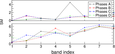
Figure 1: Second moments $\mathcal{S}_{n}$ (inverse locality) of the Wannier functions in the $n$th band, minimized by using the conjugate gradient method. Four different, randomly chosen initial sets of Bloch phases, A, B, C, D, were used for the CG optimization. Top: Sq-D crystal, TM polarization. Bottom: Tr-D crystal, TE polarization.

II.2 Conjugate gradient method

The commonly adopted way of finding maximally localized Wannier functions is to minimize the corresponding second moment $\mathcal{S}_{n}$ with respect to the set of Bloch phases $\phi_{n\mathbf{k}}$ in the $n$th band. Note that, by definition of the SM, the regions far away from the Wannier center (where the Wannier functions usually have an increasingly complex structure) contribute to the SM with quadratically increasing weight. For this optimization we first apply a standard conjugate gradient (CG) method. This method tends to get trapped in the local extrema and, hence, requires a careful choice of the initial set of Bloch phases john . In figure 1 representative examples of the locality of the SM-optimized Wannier functions are shown for Sq-D (TM polarization) and Tr-D (TE polarization) structures. Here and in the following, the Bloch modes have been calculated using the plane wave expansion method mpb-art . The minimized SM (i.e., the inverse locality) of the Wannier functions in the first eight bands are displayed for four different, random distributions of the initial Bloch phases. As expected, the optimal locality obtained using the CG method depends crucially on the choice of the initial phases. This is an indication that the SM of the Wannier functions possesses several local minima.

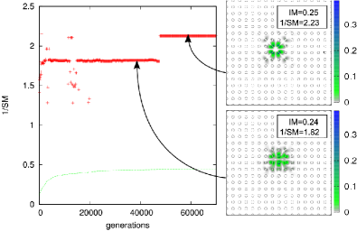
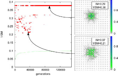
Figure 2: Locality ($1/\mathcal{S}_{n}$) of the SM-optimized Wannier functions as a function of GA generation for the Sq-D structure, TM polarization, 3rd band (top) and for the Sq-A structure, TE polarization, 5th band (bottom). The dashed, green line shows the locality of the best-localized Wannier function in each generation. Every 100 generations, these Wannier functions served as a starting point for the subsequent CG optimization step (red crosses). On the right hand side, the modulus square of the SM-optimized Wannier function is shown for an early (top: 40000th, bottom: 38300th) and a later (top: 60000th, bottom: 100000th) generation, respectively.

II.3 Genetic algorithm

The proper choice of the initial set of Bloch phases is in general not trivial john . Even if such a choice can be justified, one can never be sure that the resulting SM-optimized Wannier functions indeed correspond to the global minimum of the SM. To solve the global optimization problem and to examine the validity of the SM optimization in more detail, we have applied a global, stochastic-based optimization technique, namely a genetic algorithm (GA) method MIT99 . Taking the biologic evolution in nature as a model, the GA method works with a population of individuals which pass through a selection procedure and can reproduce themselves. Each Wannier function represents an individual. The set of Bloch phases, which determines the Wannier function, is represented as a large, binary string. The GA method starts with a population of random Wannier functions and passes them through a selection procedure where only that one half of the Wannier functions are retained which are most strongly localized with respect to the given locality criterion (“most fit individuals). In a second step, these survived individuals are allowed to reproduce themselves by randomly mixing their strings of phases, thus passing their attributes to the offsprings. Together with their off-springs, the survived individuals, which correspond to better localized Wannier functions, comprise the new generation. By iterating this procedure over several thousands of generations the algorithm will converge slowly but definitely towards the global extremum. Once the GA procedure has reached the valley of the global extremum, the CG method should be applied subsequently to the GA algorithm in order to accelerate the convergence and improve the accuracy of the solution MIT99 .

In figure 2 the evolution of the GA results is depicted for two representative systems and polarizations. Every 100 generations a Wannier function with highest locality in the current population was taken as a starting point for the subsequent CG optimization. Over the first several thousand generations the locality of the resulting Wannier functions is varying strongly, indicating hopping of the solution among different local minima due to the stochastic nature of the algorithm. At the top panel of figure 2 one can observe how the algorithm is stuck in a local minimum over several thousands of generations, before it escapes and reaches the global minimum valley at around the 50000th generation. An improvement of the locality for later generations is clearly seen from the modulus square of the optimized Wannier functions (figure 2, right panels). The discontinuous nature of the GA method ensures with stochastic certainty that the global minimum of the SM is found, providing the best localization of the Wannier functions with respect to a given locality measure. At the same time, however, the numerical load of the GA method exceeds the one of the CG method by far, making it inappropriate for routine application for an efficient construction of maximally localized Wannier functions.

III Integrated modulus optimization

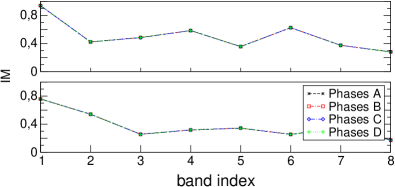
Figure 3: Locality ($\mathcal{I}_{n}$) of the Wannier functions optimized with respect to the IM locality measure using the CG method. Four different randomly chosen initial sets of Bloch phases were used for the CG optimization. Top: Sq-D crystal, TM polarization. Bottom: Tr-D crystal, TE polarization.

The complicated structure of the Wannier functions at large distances, which is expressed by several local minima of their SMs and the associated difficulties in the construction of maximally localized Wannier functions, motivates the search for a simpler criterion for the locality of Wannier functions. Here, we introduce a new criterion, the integrated modulus square (IM), defined as

$$\mathcal{I}_{n}(\{\phi_{n\mathbf{k}}\})=\int_{\text{UC}}d^{2}r\mathbf{W}_{n\mathbf{R}}^{*}(\mathbf{r})X(\mathbf{r})\mathbf{W}_{n\mathbf{R}}(\mathbf{r}),$$ (10)

where the integration region is the first unit cell (UC) around the Wannier center (UC). We choose the function $X(\mathbf{r})$ in such a way, that the IM is equal to unity for a Wannier function which is completely confined within such a unit cell. i.e.,

$$X(\mathbf{r})=\left\{\begin{array}[]{ll}\epsilon(\mathbf{r})&\quad\mbox{for TM}\\ 1&\quad\mbox{for TE}\end{array}\right.\ .$$ (11)

A well localized Wannier function corresponds to a large IM, and one needs to maximize the IM in order to obtain the maximally localized Wannier functions. The IM is a very sharp criterion, since it does not depend on the structure of the Wannier functions outside of the integration region at all.

We examined the IM locality measure as a localization criterion for the same four different physical systems and both polarizations as it was done in the SM case. To that end we construct maximally localized Wannier functions using the same four different, randomly chosen initial sets of Bloch phases as in Section II. Representative examples of CG optimization are shown in figure 3. In contrast to the SM case, the localities of the resulting Wannier functions coincide for all four sets of phases. This is the case for all considered systems and polarizations, strongly indicating that the IM locality measure does not possess any local extrema.

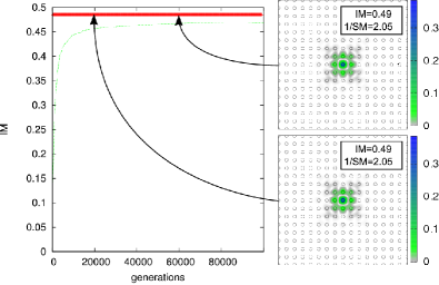
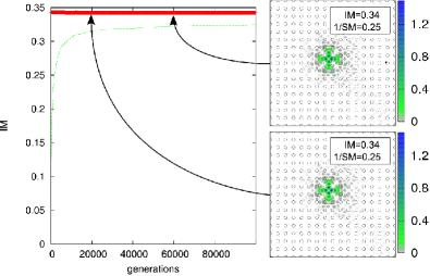
Figure 4: Locality ($\mathcal{I}_{n}$) of the IM-optimized Wannier functions as a function of GA generation for the Sq-D structure, TM polarization, 3rd band (top) and for the Sq-A structure, TE polarization, 5th band (bottom). The dashed green line shows the locality of the best-localized Wannier function in each generation. Every 100 generations these Wannier functions served as a starting point for the subsequent CG optimization step (red crosses). On the right-hand side, the modulus square of the SM-optimized Wannier functions is shown for an early (20000th) and a later (60000) generation, respectively.

To support this hypothesis, we applied the GA method to solve the optimization problem. For all considered structures no significant variation of the locality has been observed for different GA generations. Representative examples are shown in figure 4. One can clearly see, that over many thousands of generations the locality of the Wannier functions optimized with respect to IM criterion stays constant. This proves numerically that the considered optimization problem possesses a single extremum, making the procedure independent on the choice of the initial set of Bloch phases. As a consequence, the use of the IM as a locality criterion together with the CG as an optimization method represents a fast as well as reliable method for the construction of maximally localized Wannier functions. Figures 5 and 6 show the maximally localized Wannier functions for the first several bands of the Sq-D (TM polarization) and Sq-A (TE polarization) structures, respectively. In both cases the IM criterion was used along with the CG method. The optimized Wannier functions demonstrate good locality which degrades slowly with increasing band indices, since the envelope functions become more and more oscillatory, reflecting the not-plane-wave like nature of Bloch modes. It is worth noting, that the Wannier functions optimized with respect to the IM and SM criteria are in general not equal, even if the global minimum of the SM or the global maximum of the IM has been reached. For example for the system of dielectric rods in air (TM polarization) the SM- and IM-optimized Wannier functions coincide for the 1st and the 2nd band (not shown), but not for the third band (top right Wannier function in figures 2 and 4).

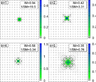
Figure 5: Modulus square of the maximally localized Wannier functions (with respect to the IM) for the Sq-D structure (TM polarization). The Wannier center was chosen as ’on-site’ for the 1st and 5th band and as ’between’ for the 2nd and 4th band.

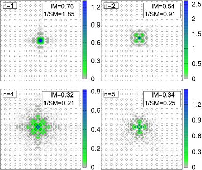
Figure 6: Modulus square of the maximally localized Wannier functions (with respect to the IM) for Sq-A structure (TE polarization). The Wannier center was chosen as ’on-site’ for the 1st band and as ’between’ for the 2nd, 4th and 5th band.

Sometimes, it is beneficial to use the time-reversal symmetry of wave operators $\mathcal{L}_{E}$ and $\mathcal{L}_{H}$ to construct real Wannier functions. This is possible, since the envelope functions of the Bloch modes transform as

$$u_{n\mathbf{-k}}(\mathbf{r})=u_{n\mathbf{k}}^{*}(\mathbf{r})$$ (12)

under time reversal (inversion of the reciprocal space), and the Bloch phases can be constrained by the condition

$$\phi_{n\mathbf{k}}=-\phi_{n\mathbf{-k}}\ .$$ (13)

By restricting the parameter space of the optimization problem in such a way, we found that both SM and IM optimization criteria possess multiple extrema, making the use of local optimization method not efficient without special choice of the initial Bloch phases. However, using real-valued Wannier functions is of advantage for the considerations of the next section.

IV Choice of initial conditions

Here we propose an analytical expression for a generic set of Bloch phases to be used as a starting point for the optimization procedure. It is based on the following theorem.

Theorem: Suppose that (i) the Wannier functions are real-valued, i.e., $\phi_{n\mathbf{k}}=-\phi_{n\mathbf{-k}}$, and the Bloch functions $\mathbf{B}_{n\mathbf{k}}(\mathbf{r})=\mathrm{e}^{\mathrm{i}\phi_{n\mathbf{k}}}\mathbf{\tilde{B}}_{n\mathbf{k}}(\mathbf{r})$ conform to the following conditions: $\text{Re}(\mathbf{B}_{n\mathbf{k}}(\mathbf{r}))$ has the same sign (i) for all points $\mathbf{r}$ in the unit cell and (ii) for all wave vectors $\mathbf{k}$ in the first Brillouin zone (for each component of the vector Bloch function). Then maximizing the IM of the Wannier functions,

$$\mathcal{I}^{W}_{n}(\{\phi_{n\mathbf{k}}\})=\int_{\text{UC}}d^{2}r\left|\mathbf{\mathbf{W}}_{n\mathbf{R}}(\mathbf{r})\right|^{2}$$ (14)

with respect to the Bloch phases $\phi_{n\mathbf{k}}$ is equivalent to maximizing the IM of the real part of the Bloch functions in the first unit cell around the Wannier center,

$$\mathcal{I}^{B}_{n}(\{\phi_{n\mathbf{k}}\})=\int_{\text{UC}}d^{2}r\left(\text{Re}(\mathrm{e}^{\mathrm{i}\phi_{\mathbf{k}}}\mathbf{\tilde{B}}_{n\mathbf{k}})\right)^{2}$$ (15)

for each wave vector in the first Brillouin zone separately. This theorem holds in any spatial dimension, even though in this paper we consider two-dimensional systems only. Note that in the above expressions we have set the weight factor $X(\mathbf{r})$ appearing in Eq. (10) equal to unity for simplicity.

The proof is straightforward. Due to the translation property of the Wannier function, (8), it is sufficient to prove the equivalence for $\mathbf{R}=\mathbf{0}$ only. In this case

$$\mathbf{W}_{n\mathbf{0}}(\mathbf{r})=\frac{1}{\sqrt{N}}\sum_{\mathbf{k}\in\text{BZ}}\mathbf{B}_{n\mathbf{k}}.$$ (16)

Figure 7: Modulus square of Bloch-criterion (Eq. 15) optimized Wannier functions for a square lattice of dielectric rods in air (TM polarization). For n=1,2,4 the Bloch criterion is equivalent to the IM-criterion for real Wannier functions. For n=3,5,6 the Wannier functions show at least a tendency to localize around the Wannier center.

It is easy to recognize that the equality

$$\int_{\text{UC}}d^{2}r\left|\text{Re}(\mathbf{W}_{n\mathbf{0}}(\mathbf{r}))\right|=\frac{1}{\sqrt{N}}\sum_{\mathbf{k}\in\text{BZ}}\int_{\text{UC}}d^{2}r\left|\text{Re}(\mathbf{B}_{n\mathbf{k}})\right|$$

holds, if the conditions (ii) and (iii) are fulfilled. Since the Wannier functions are chosen to be real-valued (i), the functional on the left-hand side is maximized by the same set of $\phi_{n\mathbf{k}}$ as $\mathcal{I}^{W}_{n}(\{\phi_{n\mathbf{k}}\})$, which proves the theorem.

The maximization problem (15) can be solved analytically leading to the following set of Bloch phases

$$\tan(2\phi_{\mathbf{k}})=\frac{-\int_{\text{UC}}d^{2}r2\text{Re}(\tilde{B}_{n\mathbf{k}})\text{Im}(\tilde{B}_{n\mathbf{k}})}{\int_{\text{UC}}d^{2}r\{\text{Re}(\tilde{B}_{n\mathbf{k}})^{2}-\text{Im}(\tilde{B}_{n\mathbf{k}})^{2}\}},$$ (17)

where $\tilde{B}_{n\mathbf{k}}=\left[\mathbf{\tilde{B}}_{n\mathbf{k}}(\mathbf{r})\cdot\mathbf{\tilde{B}}_{n\mathbf{k}}(\mathbf{r})\right]^{1/2}$ is the (complex) amplitude of the vector Bloch function. Relation (17) defines the Bloch optimization criterion. Note that the phases which are transformed by $\phi_{\mathbf{k}}\rightarrow\phi_{\mathbf{k}}+\pi$, or equivalently $\mathrm{e}^{\mathrm{i}\phi_{\mathbf{k}}}\rightarrow\mathrm{e}^{\mathrm{i}(\phi_{\mathbf{k}}+\pi)}=-\mathrm{e}^{\mathrm{i}\phi_{\mathbf{k}}}$, also fulfill (17). Furthermore, the phases which fulfill (17) also obey (13) and, therefore, the Wannier functions optimized with respect to the Bloch criterion (15) are real-valued, as initially assumed.

Due to the strongly oscillatory nature of Bloch functions in coordinate space (especially for the higher order bands), condition (ii) will hardly be fulfilled exactly in a realistic system. But the conditions (i) and (iii) can always be fulfilled simply by correct choice of the phase factor sign. In figure 7 an example of the Bloch criterion optimization is shown for the Sq-D structure (TM polarization). For the 1st, 2nd and 4th bands Bloch functions fulfill Bloch criterion conditions at least approximately, and an analytical set of Bloch phases leads to well localized Wannier functions. Even in the case when the Bloch functions do not maximize the Bloch criterion Eq. (15) exactly, the Wannier functions optimized with respect to (15) exhibit a tendency to localize around its Wannier center. The same tendency has been obtained for all four test structures in both fundamental polarizations. This suggests to use the analytical set of Bloch phases (17) as an initial set of phases for the numerical optimization, using either second moment or integrated modulus methods. This should help avoiding the local minima trapping problem and can reduce the computation time considerably.

V Wannier function quality

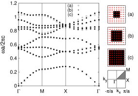
Figure 8: Band structure of a square lattice of dielectric rods in air (TM polarization). The dashed curve is the original band structure, the solid dots are the reproduced band structure obtained by within Wannier function formalism. On the right side the set of next neighboring sites surrounding Wannier center $\mathbf{R}=\mathbf{0}$ is shown for different nearest neighbor approximations.

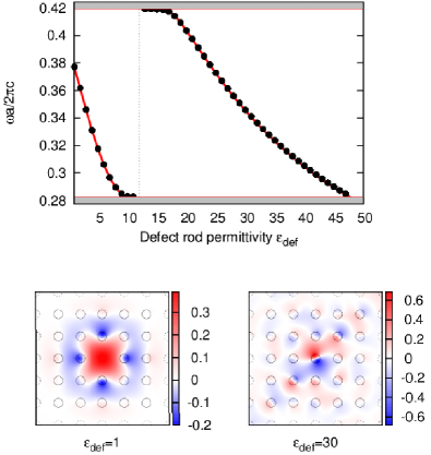
Figure 9: Frequencies of the modes in a point defect consisting of a single rod with differing permittivity $\epsilon_{def}$ in a a square lattice of dielectric rods in air (TM polarization). The dots indicate the results of the Wannier function approach by taking the first eight bands into account. They are in complete agreement with plane wave calculations (red line) mpb-art . At the bottom the real part of two defect modes with $\epsilon_{def}=1$ and $\epsilon_{def}=30$ is shown.

In this section the quality of IM optimized Wannier functions is demonstrated by using them as a basis set for photonic crystal defect structure analysis. In figure 8 the reconstructed tight-binding band structure of a square lattice of dielectric rods in air (TM polarization) is shown. The number of lattice sites taken into account in the nearest neighbor approximations were increased successively. The deviation of the reconstructed band structure from the original band structure decreases by increasing the number of next neighbors taken into account. By restricting to lattice sites separated by up to four lattice constants the band structure is reproduced well except for small deviation at higher bands and symmetry points. The slight mismatch for higher bands is due to the fact that the higher band Wannier functions are not as well localized as the lower ones.

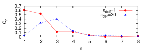
Figure 10: The band index contribution $C_{n}$ for the defect modes $\epsilon_{def}=1$ and $\epsilon_{def}=30$. Since the defect frequency lies inside the band gap between the 1st and the 2nd band, only the lower band Wannier functions contribute to the defect mode.

We further calculated the modes and frequencies of a point defect structures which consist of a single rod with deviating permittivity $\epsilon_{def}$ at $\mathbf{R}_{def}$ in the Sq-D structure. The light propagation inside the band gap between the first and the second band is forbidden and the formation of a localized defect mode is possible. We split up the total permittivity $\epsilon(\mathbf{r})=\epsilon_{p}(\mathbf{r})+\delta\epsilon(\mathbf{r}),$ into a periodic term $\epsilon_{p}(\mathbf{r})$ which corresponds to the unperturbed system, and a defect term $\delta\epsilon(\mathbf{r})=(\epsilon_{def}-\epsilon_{p})\Theta(r-|\mathbf{R}_{def}-\mathbf{r}|)$. An expansion of the $z$-component of the electric field in terms of maximally localized Wannier functions leads to a generalized eigenvalue problem with sparse matrices Busch2003 . The defect mode frequencies are obtained from the solution of this sparse system (Fig. 9). The first eight Wannier functions have been taken into account. There are monopole like defect modes for a defect rod permittivity of $\epsilon_{def}<12$ and doubly degenerated, dipole like modes for higher permittivities in the defect rod $\epsilon_{def}>12$. The results are in complete agreement with plane wave calculations mpb-art . To analyze contribution of the individual Wannier functions to the defect mode, the band index contribution

$$C_{n}=\frac{1}{M}\sum_{\mathbf{R}}|E_{n\mathbf{R}}|^{2}$$ (18)

where the normalization factor is given by $M=\sum_{n\mathbf{R}}|E_{n\mathbf{R}}|^{2}$ is shown in figure 10 for the defect modes $\epsilon_{def}=1$ and $\epsilon_{def}=30$. One can see, that $C_{n}$ rapidly decrease for higher band indices. Since the defect mode frequencies are in between the 1st and the 2nd band, only the lower band Wannier functions contribute to the defect modes. Therefore it is justified to cut of the band index which reduces the numerical load.

VI Conclusion

The procedure to construct maximally localized Wannier functions by Bloch phase optimization was analyzed for several two dimensional photonic crystals for both fundamental polarizations, using two different locality measures. Although the stochastic, genetic algorithm is numerically too costly for routine application, it has, as a global optimization method, provided us an important benchmark to judge under which conditions the faster and less memory intensive, but local conjugate gradient method finds the global optimum of a given locality measure. We found that the commonly used second moment locality measure has generically multiple extrema, which makes it difficult to construct maximally localized Wannier functions by local optimization techniques. One may conjecture that this multiplicity results from the complex oscillatory behavior of the (not yet optimized) Wannier functions at large distances from the Wannier center, which makes the dominant contribution to the second moment. This led us to propose a new locality measure which is controlled by the behavior close the Wannier center, the integrated modulus square measure. We showed numerically by comparison of conjugate gradient and genetic algorithm optimization that this measure does not feature multiple extrema and is, therefore, suitable for fast and efficient local optimization techniques, like the standard conjugate gradient method. Because this result presumably originates from the local nature of the integrated modulus measure, it should hold generally, not only for two-dimensional systems, but also in three dimensions for photonic as well as electronic lattices.

We also presented and tested an analytical formula for the set of Bloch phases to be used as a starting point of the optimization process. This initial set of Bloch phases is suggested because, albeit it does not solve the optimization problem in general, it does generate maximally localized Wannier functions in special cases where the optimization problem can be solved analytically. We expect that these two main results may significantly increase the efficiency of the Wannier function approach for the description of defect structures in photonic lattices.

This work was supported in part by the Deutsche Forschungsgemeinschaft (FOR 557).

References

- (1) K. Sakoda, Optical Properties of Photonic Crystals (Springer, 2001).
- (2) A. Taflove and S. C. Hagnes, Computational Electrodynamics: The Finite-Difference Time-Domain Method (Artech House, 2000).
- (3) C. A. J. Fletcher, Computational Galerkin Methods (Springer, 1984).
- (4) D. N. Chigrin, “Spatial distribution of the emission intensity in a photonic crystal: Self-interference of Bloch eigenwaves,” Physical Review A 79, 1–9 (2009).
- (5) C. Kremers, D. N. Chigrin, and J. Kroha, “Theory of Cherenkov radiation in periodic dielectric media: Emission spectrum,” Physical Review A 79, 1–10 (2009).
- (6) C. Kremers and D. N. Chigrin, “Spatial distribution of Cherenkov radiation in periodic dielectric media,” Journal of Optics A: Pure and Applied Optics 11, 114008 (2009).
- (7) K. M. Leung, “Defect modes in photonic band structures - a green-function approach using vector wannier functions,” J. Opt. Soc. Am. B-Opt. Phys. 10, 303–306 (1993).
- (8) E. Lidorikis, M. M. Sigalas, E. N. Economou, and C. M. Soukoulis, “Tight-binding parametrization for photonic band gap materials,” Phys. Rev. Lett. 81, 1405–1408 (1998).
- (9) J. Albert, C. Jouanin, D. Cassagne, and D. Bertho, “Generalized wannier function method for photonic crystals,” Phys. Rev. B 61, 4381–4384 (2000).
- (10) J. Albert, C. Jouanin, D. Cassagne, and D. Monge, “Photonic crystal modelling using a tight-binding wannier function method,” Opt. Quantum Electron. 34, 251–263 (2002).
- (11) N. Marzari and D. Vanderbilt, “Maximally localized generalized Wannier functions for composite energy bands,” Phys. Rev. B 56, 12847 (1997).
- (12) I. Souza, N. Marzari, and D. Vanderbilt, “Maximally localized Wannier functions for entangled energy bands,” Phys. Rev. B 65, 035109 (2002).
- (13) D. M. Whittaker and M. P. Croucher, “Maximally localized Wannier functions for photonic lattices,” Phys. Rev. B 67, 085204 (2003).
- (14) A. Garcia-Martin, D. Hermann, F. Hagmann, K. Busch, and P. Wölfle, “Defect computations in photonic crystals: a solid state theoretical approach,” Nanotechnology 14, 177 (2003).
- (15) K. Busch, S. Mingaleev, A. Garcia-Martin, M. Schillinger, and D. Hermann, “The wannier function approach to photonic crystal circuits,” J. Phys.-Condes. Matter 15, R1233–R1256 (2003).
- (16) Y. Jiao, S. Mingaleev, M. Schillinger, D. Miller, S. Fan, and K. Busch, “Wannier basis design and optimization of a photonic crystal waveguide crossing,” IEEE Photonics Technol. Lett. 17, 1875–1877 (2005).
- (17) E. Istrate and E. H. Sargent, “Photonic crystal heterostructures and interfaces,” Rev. Mod. Phys. 78, 455–481 (2006).
- (18) A. McGurn, “Impurity mode techniques applied to the study of light sources,” J. Phys. D-Appl. Phys. 38, 2338–2352 (2005).
- (19) H. Takeda, A. Chutinan, and S. John, “Localized light orbitals: Basis states for three-dimensional photonic crystal microscale circuits,” Phys. Rev. B 74 (2006).
- (20) J. des Cloizeaux, “Analytical properties of -dimensional energy bands and Wannier functions,” Phys. Rev. A 135, 698 (1964).
- (21) H. Takeda, A. Chutinan, and S. John, “Localized light orbitals: Basis states for three-dimensional photonic microscale circuits,” Phys. Rev. B 74, 195116 (2006).
- (22) K. Busch, S. F. Mingaleev, A. Garcia-Martin, M. Schillinger, and D. Hermann, “Wannier function approach to photonic crystal circuits,” Journal of Physics: Condensed Matter 15, R1233 (2003).
- (23) S. G. Johnson and J. D. Joannopoulos, “Block-iterative frequency-domain methods for maxwell’s equations in a planewave basis,” Opt. Express 8, 173–190 (2001).
- (24) M. Mitchell, An Introduction to Genetic Algorithms (MIT Press, Cambridge, 1999).