The unification of inflation and late-time acceleration in the frame of $k$-essence

Abstract

By using the formulation of the reconstruction, we explicitly construct models of $k$-essence, which unify the inflation in the early universe and the late accelerating expansion of the present universe by a single scalar field. Due to the higher derivative terms, the solution describing the unification can be stable in the space of solutions, which makes the restriction for the initial condition relaxed. The higher derivative terms also eliminate tachyon. Therefore we can construct a model describing the time development, which cannot be realized by a usual inflaton or quintessence models of the canonical scalar field due to the instability or the existence of tachyon. We also propose a mechanism of the reheating by the quantum effects coming from the variation of the energy density of the scalar field.

I Introduction

We now believe the accelerating expansion of the present universe by several cosmological observations WMAP1 ; Komatsu:2008hk ; SN1 ; Astier:2005qq . The acceleration has been often supposed to be generated by the dark energy, which is an unknown fluid. So-called $k$-essence model Chiba:1999ka ; ArmendarizPicon:2000dh ; ArmendarizPicon:2000ah is a model of the dark energy. The $k$-essence model is originated from $k$-inflation model ArmendarizPicon:1999rj ; Garriga:1999vw . It is possible to regard the tachyon dark energy model Sen:2002nu ; Sen:2002an ; Gibbons:2002md ; Bagla:2002yn , ghost condensation model ArkaniHamed:2003uy ; ArkaniHamed:2003uz , and scalar field quintessence model Peebles:1987ek ; Ratra:1987rm ; Chiba:1997ej ; Zlatev:1998tr as variations of the $k$-essence model.

Since the $k$-essence model is originated from $k$-inflation model, it might be natural to consider a model unifying the inflation and the late acceleration by a single scalar field. In this paper, we try to construct such models by using the formulation of the reconstruction Nojiri:2006be ; Elizalde:2008yf ; Nojiri:2009fq ; Nojiri:2009kx ; Matsumoto:2010uv ; Nojiri:2010wj and we also propose a mechanism of the reheating by the quantum effects. In the models, the solution which describes the unification of the inflation and the late acceleration can be stable in the space of solutions and also there does not appear tachyon due to the higher derivative terms. This tells that we can construct a model describing the time development, which cannot be realized by models of usual canonical scalar field like inflaton or quintessence due to the instability or the existence of tachyon.

II Review of the reconstruction and the stability of the solution

In this section, based on Nojiri:2010wj , we review on the reconstruction by using e-folding $N$, which will be defined in this section, and discuss the stability of the solution in the space of solutions. A formulation of the reconstruction using the cosmological time has been given in Matsumoto:2010uv (about the reconstruction of the canonical/phantom scalar field, see Nojiri:2005pu ; Capozziello:2005tf and about the general formalism of the reconstruction, see Nojiri:2006be ; Elizalde:2008yf ; Nojiri:2009fq ; Nojiri:2009kx ; Matsumoto:2010uv ; Nojiri:2010wj ). In the formulation using the cosmological time Matsumoto:2010uv , it is troublesome and difficult to discuss about the stability of the solution when matters are included. In the formulation using the e-folding $N$, as long as the $N$-dependence of the matters are known, which is often true as we will see, it is easy to construct a model where the solution is stable.

We now consider a rather general model, whose action is given by

$$S=\int d^{4}x\sqrt{-g}\left(\frac{R}{2\kappa^{2}}-K\left(\phi,X\right)+L_{\mathrm{matter}}\right)\,,\quad X\equiv\partial^{\mu}\phi\partial_{\mu}\phi\,.$$ (1)

Here $\phi$ is a scalar field. Now the Einstein equation has the following form:

$$\frac{1}{\kappa^{2}}\left(R_{\mu\nu}-\frac{1}{2}g_{\mu\nu}R\right)=-K\left(\phi,X\right)g_{\mu\nu}+2K_{X}\left(\phi,X\right)\partial_{\mu}\phi\partial_{\nu}\phi+T_{\mu\nu}\,.$$ (2)

Here $K_{X}\left(\phi,X\right)\equiv\partial K\left(\phi,X\right)/\partial X$ and $T_{\mu\nu}$ is the energy-momentum tensor of the matters. On the other hand, the variation of $\phi$ gives

$$0=-K_{\phi}\left(\phi,X\right)+2\nabla^{\mu}\left(K_{X}\left(\phi,X\right)\partial_{\mu}\phi\right)\,.$$ (3)

Here $K_{\phi}\left(\phi,X\right)\equiv\partial K\left(\phi,X\right)/\partial\phi$ and we have assumed that the scalar field $\phi$ does not directly couple with the matter.

We now assume the FRW universe whose spacial part is flat:

$$ds^{2}=-dt^{2}+a(t)^{2}\sum_{i=1,2,3}(dx^{i})^{2}\,,$$ (4)

and the scalar field $\phi$ only depends on time. Then the FRW equations are given by

$$\frac{3}{\kappa^{2}}H^{2}=2X\frac{\partial K\left(\phi,X\right)}{\partial X}-K\left(\phi,X\right)+\rho_{\mathrm{matter}}(t)\,,\quad-\frac{1}{\kappa^{2}}\left(2\dot{H}+3H^{2}\right)=K\left(\phi,X\right)+p_{\mathrm{matter}}(t)\,.$$ (5)

It is often convenient to use redshift $z$ instead of cosmological time $t$ since the redshift has direct relation with observations (see Nojiri:2009kx for the reconstruction of $F(R)$ gravity using the redshift $z$). The redshift is defined by

$$a(t)=\frac{a\left(t_{0}\right)}{\left(1+z\right)}=\mathrm{e}^{N-N_{0}}\,.$$ (6)

Here $t_{0}$ is the cosmological time of the present universe, $N_{0}$ could be an arbitrary constant, and $N$ is called as e-folding and directly related with the redshift $z$. In terms of $N$, the FRW equations (5) can be rewritten as

$$\frac{3}{\kappa^{2}}H^{2}=2X\frac{\partial K\left(\phi,X\right)}{\partial X}-K\left(\phi,X\right)+\rho_{\mathrm{matter}}(N)\,,\quad-\frac{1}{\kappa^{2}}\left(2HH^{\prime}+3H^{2}\right)=K\left(\phi,X\right)+p_{\mathrm{matter}}(N)\,.$$ (7)

Here $H^{\prime}\equiv dH/dN$. If the matters have constant EoS parameters $w_{i}$, the energy density of the matters is given by

$$\rho_{\mathrm{matter}}(N)=\sum_{i}\rho_{0i}a^{-3(1+w_{i})}=\sum_{i}\rho_{0i}\mathrm{e}^{-3(1+w_{i})\left(N-N_{0}\right)}\,,$$

$$p_{\mathrm{matter}}(N)=\sum_{i}w_{i}\rho_{0i}a^{-3(1+w_{i})}=\sum_{i}w_{i}\rho_{0i}\mathrm{e}^{-3(1+w_{i})\left(N-N_{0}\right)}\,.$$ (8)

Here $\rho_{0i}$’s are constants. Eq. (II) tells the $N$ dependence of the matter energy density $\rho_{\mathrm{matter}}$ is explicitly given. Note that the $N$ dependence is not so clear when the matters are created or annihilated as in the period of the reheating but in the periods of the inflation and the late acceleration, the expression of $\rho_{\mathrm{matter}}$ in (II) could be valid. For the general energy density of matters $\rho_{\mathrm{matter}}(N)$, since the conservation law

$$\dot{\rho}_{\mathrm{matter}}+3H\left(\rho_{\mathrm{matter}}+p_{\mathrm{matter}}\right)=0\,,$$ (9)

can be rewritten in terms of $N$ as

$$\rho_{\mathrm{matter}}^{\prime}(N)+3\left(\rho_{\mathrm{matter}}(N)+p_{\mathrm{matter}}(N)\right)=0\,,$$ (10)

we find

$$p_{\mathrm{matter}}(N)=-\rho_{\mathrm{matter}}(N)-\frac{1}{3}\rho_{\mathrm{matter}}^{\prime}(N)\,.$$ (11)

Then we can rewrite the FRW equations (7) as

$$K\left(\phi,X\right)=-\frac{1}{\kappa^{2}}\left(2H\frac{dH}{dN}+3H^{2}\right)+\rho_{\mathrm{matter}}(N)+\frac{1}{3}\rho_{\mathrm{matter}}^{\prime}(N)\,,\quad-X\frac{\partial K\left(\phi,X\right)}{\partial X}=\frac{1}{\kappa^{2}}H\frac{dH}{dN}-\frac{1}{6}\rho_{\mathrm{matter}}^{\prime}(N)\,.$$ (12)

If we define a new variable $G(N)=H(N)^{2}$, the equations in (12) have the following forms:

$$K\left(\phi,X\right)=-\frac{1}{\kappa^{2}}\left(G^{\prime}(N)+3G(N)\right)+\rho_{\mathrm{matter}}(N)+\frac{1}{3}\rho_{\mathrm{matter}}^{\prime}(N)\,,\quad-X\frac{\partial K\left(\phi,X\right)}{\partial X}=\frac{1}{2\kappa^{2}}G^{\prime}(N)-\frac{1}{6}\rho_{\mathrm{matter}}^{\prime}(N)\,.$$ (13)

Then by using the appropriate function $g_{\phi}(\phi)$, if we choose

$$K(\phi,X)=\sum_{n=0}^{\infty}\left(\frac{X}{g_{\phi}(\phi)+\frac{\kappa^{2}}{3}\rho_{\mathrm{matter}}(\phi)}+1\right)^{n}\tilde{K}^{(n)}(\phi)\,,$$

$$\tilde{K}^{(0)}(\phi)\equiv-\frac{1}{\kappa^{2}}\left(g_{\phi}^{\prime}(\phi)+3g_{\phi}(\phi)\right)\,,\quad\tilde{K}^{(1)}(\phi)=\frac{1}{2\kappa^{2}}g_{\phi}^{\prime}(\phi)\,,$$ (14)

we find the following solution for the FRW equations (5),

$$G(N)=H(N)^{2}=g_{\phi}(N)+\frac{\kappa^{2}}{3}\rho_{\mathrm{matter}}(N)\,,\quad\phi=N\quad\left(X=-H^{2}\right)\,.$$ (15)

Now $\tilde{K}^{(n)}(\phi)$ with $n\geq 2$ can be arbitrary. As we will see, $\tilde{K}^{(2)}(\phi)$ is related with the stability of the solution and the existence of tachyon although $\tilde{K}^{(n)}(\phi)$ with $n\geq 2$ does not affect the development of the expansion of the universe.

We should note that the solution (15) is merely one of solutions of the FRW equations (12) in the model given by (II). In order that the solution (15) could be surely realized, the solution (15) should be stable under the perturbation in the space of solutions of the FRW equations. We now write the perturbation from the solution (15) as follows,

$$G(N)=G_{0}(N)+\delta G(N)\quad\left(G_{0}(N)\equiv g_{\phi}(N)+\frac{\kappa^{2}}{3}\rho_{\mathrm{matter}}(N)\right)\,,\quad\phi=N+\delta\phi(N)\,.$$ (16)

We should note that in many cases, the $N$-dependence in the energy density $\rho_{\mathrm{matter}}$ of matter is usually given by a fixed function as in (II) and therefore we find $\delta\rho_{\mathrm{matter}}=0$. Then the equations in (13) gives,

$$-\frac{1}{\kappa^{2}}\left(g_{\phi}^{\prime\prime}(N)+3g_{\phi}^{\prime}(N)\right)\delta\phi(N)-\frac{g_{\phi}^{\prime}(N)}{2\kappa^{2}}\left(\frac{\delta G(N)}{G_{0}(N)}+2\delta\phi^{\prime}(N)-\frac{G_{0}^{\prime}(N)}{G_{0}(N)}\delta\phi(N)\right)=-\frac{1}{\kappa^{2}}\left(\delta G^{\prime}(N)+3\delta G(N)\right)\,,$$

$$\frac{1}{\kappa^{2}}g_{\phi}^{\prime}(N)\delta\phi^{\prime}(N)+\frac{g_{\phi}^{\prime}(N)}{2\kappa^{2}}\frac{\delta G(N)}{G_{0}(N)}+\frac{g_{\phi}^{\prime\prime}(N)}{2\kappa^{2}}\delta\phi(N)-\frac{g_{\phi}^{\prime}(N)}{2\kappa^{2}}\frac{G_{0}^{\prime}(N)}{G_{0}(N)}\delta\phi(N)$$

$$-2\tilde{K}^{(2)}(N)\left(\frac{\delta G(N)}{G_{0}(N)}+2\delta\phi^{\prime}(N)-\frac{G_{0}^{\prime}(N)}{G_{0}(N)}\delta\phi(N)\right)=\frac{1}{2\kappa^{2}}\delta G^{\prime}(N)\,.$$ (17)

Then we find

$$\left(\begin{array}[]{c}\delta\phi^{\prime}(N)\\ \delta G^{\prime}(N)\end{array}\right)=\frac{1}{L(N)}\left(\begin{array}[]{cc}A&B\\ C&D\end{array}\right)\left(\begin{array}[]{c}\delta\phi(N)\\ \delta G(N)\end{array}\right)\,,$$ (24)

$$A\equiv 3g_{\phi}^{\prime}(N)+\frac{G_{0}^{\prime}(N)}{2G_{0}(N)}L(N)\,,\quad B\equiv-3-\frac{L(N)}{2G_{0}(N)}\,,$$

$$C\equiv\left(g_{\phi}^{\prime\prime}(N)+3g_{\phi}^{\prime}(N)\right)L(N)+3g_{\phi}^{\prime}(N)^{2}\,,\quad D\equiv-3L(N)-3g_{\phi}^{\prime}(N)\,.$$ (25)

Here

$$L(N)\equiv g_{\phi}^{\prime}(N)-8\kappa^{2}\tilde{K}^{(2)}(N)\,.$$ (26)

In order for the solution (15) to be stable, the perturbations $\delta\phi(N)$ and $\delta G(N)$ should decrease with the increase of $N$, which requires that the real parts of the eigenvalues for the matrix $\left(\begin{array}[]{cc}A&B\\ C&D\end{array}\right)$ should be negative. Therefore the stability of the solution requires $A+D<0$ and $AD-BC>0$, which gives

$$3>\frac{G_{0}^{\prime}(N)}{2G_{0}(N)}\,,$$ (27)

$$\left(2G_{0}(N)+3L(N)\right)g_{\phi}^{\prime\prime}(N)+\left(g_{\phi}^{\prime}(N)-G_{0}^{\prime}(N)+L(N)\right)g_{\phi}^{\prime}(N)-L(N)G_{0}^{\prime}(N)>0\,.$$ (28)

We can find $\dot{H}<3H^{2}$ from (27), which is always satisfied when the universe is in the non-phantom phase, where $\dot{H}\leq 0$. For later convenience, we rewrite (28) in the following form:

$$H^{2}\tilde{K}^{(1)\prime}(N)-2HH^{\prime}\tilde{K}^{(1)}(N)+3\kappa^{2}\tilde{K}^{(1)}(N)\tilde{K}^{(1)\prime}(N)+2\left(\tilde{K}^{(1)}(N)\right)^{2}$$

$$+\left(4HH^{\prime}-12\kappa^{2}\tilde{K}^{(1)\prime}(N)-4\kappa^{2}\tilde{K}^{(1)}(N)\right)\tilde{K}^{(2)}(N)>0\,.$$ (29)

The condition (28) or (II) can be satisfied by choosing $L(N)$ and therefore $\tilde{K}^{(2)}(N)$ properly.

In case of usual inflaton or quintessence model, where $\tilde{K}^{(n)}(\phi)=0$ $\left(n\geq 2\right)$ in (II), there appears tachyon if the potential is concave downwards and therefore the system becomes unstable. We now show that the development of the expansion in the universe generated by the concave potential in case of the inflaton or quintessence model can be realized without tachyon by adjusting $\tilde{K}^{(2)}(\phi)$ in the $k$-essence models in this paper.

We now consider the perturbation of only scalar field $\phi$ from the solution (15) as

$$\phi=N+\delta\phi(x^{i})\,.$$ (30)

Different from the case of (16), we assume $\delta\phi$ only depends on the spacial coordinate $x^{i}$ since we are now interested in the pole of the scalar field propagator for the spacial momentum, corresponding to tachyon. Then by using (3) and (II), we obtain

$$0 = -2\frac{\tilde{K}^{(1)}(N)}{H^{2}a^{2}}\triangle\left(\delta\phi\right)+2\left\{\frac{1}{2}{\tilde{K}^{(0)^{\prime\prime}}}(N)+\tilde{K}^{(1)^{\prime\prime}}(N)+\left(3-\frac{H^{\prime}}{H}\right){\tilde{K}^{(1)^{\prime}}}(N)+\left(-\frac{H^{\prime\prime}}{H}+\left(\frac{H^{\prime}}{H}\right)^{2}-\frac{6H^{\prime}}{H}\right)\tilde{K}^{(1)}(N)\right.$$ (31)

$$\left.+\left(-4\left(\frac{H^{\prime}}{H}\right)^{2}+\frac{4H^{\prime\prime}}{H}+\frac{12H^{\prime}}{H}\right)\tilde{K}^{(2)}(N)+\frac{4H^{\prime}}{H}{\tilde{K}^{(2)^{\prime}}}(N)\right\}\delta\phi\,.$$

Here $\triangle$ is the Laplacian for the spacial coordinates $x^{i}$. Then if

$$\frac{1}{\tilde{K}^{(1)}(N)}\left\{-\frac{H^{\prime}}{H}\tilde{K}^{(1)\prime}(N)+\left(-\frac{H^{\prime\prime}}{H}+\left(\frac{H^{\prime}}{H}\right)^{2}-\frac{6H^{\prime}}{H}\right)\tilde{K}^{(1)}(N)\right.$$

$$\left.+\left(-4\left(\frac{H^{\prime}}{H}\right)^{2}+\frac{4H^{\prime\prime}}{H}+\frac{12H^{\prime}}{H}\right)\tilde{K}^{(2)}(N)+\frac{4H^{\prime}}{H}{\tilde{K}^{(2)\prime}}(N)\right\}\leq 0\,,$$ (32)

there does not appear tachyon. If we assume $\tilde{K}^{(1)}(N)<0$, which corresponds to non-phantom universe, and define $\tilde{k}^{(2)}(N)$ by

$$\tilde{K}^{(2)}(N)=H\left(a^{3}H^{\prime}\right)^{-1}\tilde{k}^{(2)}(N)\,,$$ (33)

Eq. (II) gives

$$\left.\frac{d\tilde{k}^{(2)}}{d\phi}\right|_{\phi=N}\geq\frac{a^{3}}{4}\left\{\frac{H^{\prime}}{H}{\tilde{K}^{(1)^{\prime}}}(N)-\left(-\frac{H^{\prime\prime}}{H}+\left(\frac{H^{\prime}}{H}\right)^{2}-\frac{6H^{\prime}}{H}\right)\tilde{K}^{(1)}(N)\right\}\,.$$ (34)

Then if (28) or (II) and (II) or (34) are satisfied simultaneously without divergence, we obtain a stable model without tachyon.

III Models unifying the inflation and the accelerating expansion

In this section, we propose models unifying the inflation in the early universe and the accelerating expansion in the present universe.

In (15), $g_{\phi}(N)$ corresponds to the energy density $\rho_{\phi}$ of the scalar field $\phi$:

$$\rho_{\phi}(N)=\frac{3}{\kappa^{2}}g_{\phi}(N)=2X\frac{\partial K\left(\phi,X\right)}{\partial X}-K\left(\phi,X\right)\,.$$ (35)

We expect that the energy density $\rho_{\phi}$ would behave as the cosmological constant in the period of the inflation and the late acceleration. Then we expect the behavior of $\rho_{\phi}$ as in FIG. 1. We consider the model that the particle production and the reheating would occur after the inflation.

Figure 1: The expected behavior of $\rho_{\phi}(N)$.

We now assume

1. The energy scale of inflation should be almost equal to the GUT scale.

2. Except the period of the particle production, the EoS parameter $w_{\phi}$ for the scalar field $\phi$ could be given by

   $$w_{\phi}(N)=-1-\frac{\rho_{\phi}^{\prime}(N)}{3\rho_{\phi}(N)}\,.$$ (36)

3. In general, there are two solutions $N=N_{1}$, $N_{2}$ $\left(N_{1}<N_{2}\right)$ in the equation

   $$\frac{\left.\rho_{\phi}^{\prime}\right|_{N=N_{1,2}}}{\left.\rho_{\phi}^{\prime}\right|_{\mathrm{max}}}=\frac{1}{\mathrm{e}}\,.$$ (37)

   We expect that the expression (36) could become invalid when $N_{1}<N<N_{2}$.

4. The inflation started at $N=0$ and the end of the inflation is defined by $N=N_{\mathrm{I}}\equiv N_{1}\simeq 60$.

5. The reheating and the particle production could have occurred when $N_{1}\lesssim N\lesssim N_{2}$.

6. The reheating temperature $T_{\mathrm{RH}}$ could be $10\,\mathrm{MeV}<T_{\mathrm{RH}}<10^{14}\mathrm{GeV}$.

Furthermore, the cosmological observations tell, at present, 1) the energy density of the dark energy is about $10^{-47}\,\mathrm{GeV}^{4}$, 2) the temperature of the present universe is $2.725\,\mathrm{K}$ and that at the epoch of the decoupling is almost $3000\,\mathrm{K}$ $\left(0.26\,\mathrm{eV}\right)$, which give the following constraints

$$1. \rho_{\phi}(N=0)\simeq 10^{60}\,\mathrm{GeV}^{4}\,,$$ (38)

$$2. \rho_{\phi}(N=N_{0})\simeq 10^{-47}\,\mathrm{GeV}^{4}\,,$$

$$3. w_{\phi}=-1.023\pm 0.144\quad\mbox{at $N_{0}$}\,.$$

Here we choose $N_{0}$ as the e-folding at present universe and the third constraint in (38) comes from SuperNova Legacy Survey (SNLS) date Astier:2005qq .

We should note that in the period of the reheating and/or particle production, it is difficult to apply the formulation of the reconstruction since the matter energy density is not always given by an explicit function of the e-folding $N$. In this paper, we approximate the behavior of $\rho_{\phi}$ in the period of the reheating and/or the particle production by the interpolation from the behaviors in the period of the inflation and that after the reheating.

III.1 Model 1

We now consider the following model as model 1:

$$\rho_{\phi}(N)=M^{4}\exp{\left(-\frac{1}{d^{-1}+c_{1}\exp{\left(-\frac{N-N_{\mathrm{I}}}{\Delta_{1}}\right)}}\right)}\,,$$ (39)

which gives

$$\rho_{\phi}^{\prime}(N)=-\frac{1}{c_{1}\Delta_{1}}\frac{\exp{\left(-\frac{N-N_{\mathrm{I}}}{\Delta_{1}}\right)}}{\left((c_{1}d)^{-1}+\exp{\left(-\frac{N-N_{\mathrm{I}}}{\Delta_{1}}\right)}\right)^{2}}\rho_{\phi}(N)\,.$$ (40)

Here $c_{1}$, $d$, and $\Delta_{1}$ are constants and we choose $c_{1}\simeq 6.309$ and $M\simeq 10^{15}\mathrm{GeV}$. Then the assumptions mentioned above and the constraints (38) give

$$1. \ d\gg 2\,,$$ (41)

$$2. \ \exp{\left(-\frac{1}{d^{-1}+c_{1}\exp{\left(\frac{N_{\mathrm{I}}}{\Delta_{1}}\right)}}\right)}\simeq 1\,,$$

$$3. \ d\simeq 107\ln 10\left[1-107\ln 10\cdot c_{1}\exp{\left({-\frac{(N_{0}-N_{\mathrm{I}})}{\Delta_{1}}}\right)}\right]^{-1}\,,$$

$$4. \ d\leq\frac{1}{c_{1}}\left(\sqrt{\frac{1}{0.363c_{1}\Delta_{1}}\exp{\left({-\frac{N_{0}-N_{\mathrm{I}}}{\Delta_{1}}}\right)}}-\exp{\left({-\frac{N_{0}-N_{\mathrm{I}}}{\Delta_{1}}}\right)}\right)^{-1}\,.$$

Since the scale factor $a$ is proportional to the inverse temperature $a=\mathrm{e}^{N-N_{0}}\propto T^{-1}$, we find

$$\mathrm{e}^{N-N_{\mathrm{I}}}=\frac{a(N)}{a(N_{\mathrm{I}})}\simeq\frac{a(N)}{a(N_{\mathrm{RH}})}\simeq\frac{T_{\mathrm{RH}}}{T}\,,$$ (42)

and therefore

$$N_{0}-N_{\mathrm{I}}\simeq\ln\left(\frac{T_{\mathrm{RH}}}{3\times 10^{-4}\,\mathrm{eV}}\right)=24\mbox{--}61\quad\mathrm{for}\quad T_{\mathrm{RH}}=10\,\mathrm{MeV}\mbox{--}10^{14}\,\mathrm{GeV}\,.$$ (43)

The second constraint in (41) tells that the parameter $d$ is expressed by the another parameter $\Delta_{1}$, so in this model there remains only one undetermined parameter. Then in case $T_{\mathrm{RH}}=10\,\mathrm{MeV}$, we find $(0,246.4)<(\Delta_{1},d)<(1.81,247)$ and in case $T_{\mathrm{RH}}=10^{14}\,\mathrm{GeV}$, $(0,246.4)<(\Delta_{1},d)<(4.97,248.2)$.

Now the reconstructed action has the following form:

$$K(\phi,X) = \frac{3\tilde{K}^{(1)}}{\kappa^{2}\left(\rho_{\phi}(\phi)+\rho_{m}(\phi)\right)}X+\tilde{K}^{(0)}+\tilde{K}^{(1)}+\sum_{n=2}^{\infty}\left(\frac{X}{\frac{\kappa^{2}}{3}\rho_{\phi}(\phi)+\frac{\kappa^{2}}{3}\rho_{m}(\phi)}+1\right)^{n}\tilde{K}^{(n)}(\phi)\,,$$

$$\tilde{K}^{(0)}(\phi) = -M^{4}\exp{\left(-\frac{1}{d^{-1}+c_{1}\exp{\left(-\frac{N-N_{\mathrm{I}}}{\Delta_{1}}\right)}}\right)}\left(1-\frac{\exp{\left(-\frac{N-N_{\mathrm{I}}}{\Delta_{1}}\right)}}{3c_{1}\Delta_{1}\left((c_{1}d)^{-1}+\exp{\left(-\frac{N-N_{\mathrm{I}}}{\Delta_{1}}\right)}\right)^{2}}\right)\,,$$

$$\tilde{K}^{(1)}(\phi) = -M^{4}\exp{\left(-\frac{1}{d^{-1}+c_{1}\exp{\left(-\frac{N-N_{\mathrm{I}}}{\Delta_{1}}\right)}}\right)}\frac{\exp{\left(-\frac{N-N_{\mathrm{I}}}{\Delta_{1}}\right)}}{6c_{1}\Delta_{1}\left((c_{1}d)^{-1}+\exp{\left(-\frac{N-N_{\mathrm{I}}}{\Delta_{1}}\right)}\right)^{2}}\,.$$ (44)

In order to find the constraints for $\tilde{K}^{(2)}(\phi)$ or $\tilde{k}^{(2)}(\phi)$ given by (28) or (II) and (II) or (34), we assume

$$\rho_{m}(N)\simeq\begin{cases}0&\text{for $0\leq N\leq N_{\mathrm{I}}$}\\ \rho_{m0}\mathrm{e}^{-4(N-N_{0})}&\text{for $N\geq N_{\mathrm{RH}}\simeq N_{2}$,}\end{cases}$$

$$\rho_{m0}\simeq 8.4\times 10^{-52}\mathrm{GeV}^{4}\,\ .$$ (45)

Here $N_{\mathrm{RH}}$ expresses the e-folding number when the reheating finished. Then, we obtain approximate constraints for $\tilde{k}^{(2)}(\phi)$ and $\tilde{k}^{(2)\prime}(\phi)$ for model 1 as shown in FIGs. 2–7 and we can find that there exists $\tilde{k}^{(2)}(\phi)$ or $\tilde{K}^{(2)}(\phi)$ which satisfies the constraints and does not have divergence nor vanish.

In FIG. 2, the region satisfying the constraint (II) is depicted by the directions of arrows. When $N_{\mathrm{I}}=N_{1}<N<N_{2}\simeq N_{\mathrm{RH}}$, we could not be able to use the formulation of the reconstruction due to the particle creation. The region $0<N<N_{\mathrm{I}}$ in FIG. 2 is magnified in FIG. 3 and the region $N>N_{2}\simeq N_{\mathrm{RH}}$ in FIG. 4. The region that $\tilde{k}^{(2)\prime}(N)$ of model 1 satisfies the constraint (34) is depicted in FIG. 4 and regions $0<N<N_{\mathrm{I}}$ and $N>N_{2}\simeq N_{\mathrm{RH}}$ in FIG. 4 are magnified in FIG. 5 and FIG. 6, respectively. Then we may find that we can always obtain an action where the solution becomes stable and does not have tachyon.

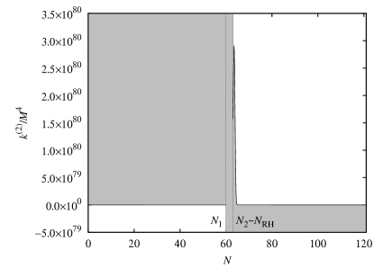
Figure 2: The regions satisfying the constraint (II) for $\tilde{k}^{(2)}(N)$ of model 1. The gray regions express the forbidden regions for the instability of the solution. In the interval $N_{\mathrm{I}}=N_{1}<N<N_{2}\simeq N_{\mathrm{RH}}$, the formulation of the reconstruction could not be applied due to the particle creation.

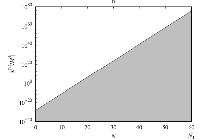
Figure 3: The region $0<N<N_{\mathrm{I}}$ in FIG. 2 is magnified. The vertical axis expresses the absolute value of $\tilde{k}^{(2)}(N)$. The symbol ‘n’ means the value of $\tilde{k}^{(2)}(N)$ is negative there.

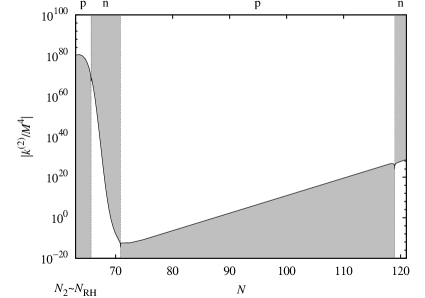
Figure 4: The regions $N>N_{\mathrm{RH}}$ in FIG. 2 are magnified. The vertical axis expresses the absolute value of $\tilde{k}^{(2)}(N)$. The symbol ‘p’ means the value of $\tilde{k}^{(2)}(N)$ is positive there.

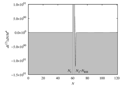
Figure 5: The regions satisfying the constraint (34) for $\tilde{k}^{(2)\prime}(N)$ of model 1. The gray regions express the regions forbidden by the constraint (34).

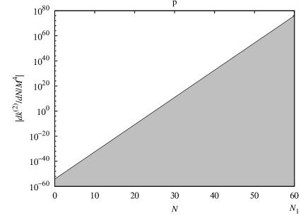
Figure 6: The region $0<N<N_{\mathrm{I}}$ in FIG. 5 is magnified. .

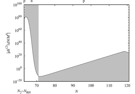
Figure 7: The regions $N>N_{\mathrm{RH}}$ in FIG. 5 are magnified. The vertical axis expresses the absolute value of $\tilde{k}^{(2)\prime}(N)$.

III.2 Model 2

As a second model, which we call as model 2, we consider the following:

$$\rho_{\phi}(N)=\frac{A}{c_{2}\exp{\left(\frac{N-N_{\mathrm{I}}}{\Delta_{2}}\right)}+1}+B\left(N+b\right)^{-\beta}\,,$$ (46)

which gives

$$\rho_{\phi}^{\prime}(N)=-\frac{Ac_{2}\exp{\left(\frac{N-N_{\mathrm{I}}}{\Delta_{2}}\right)}}{\left(c_{2}\exp{\left(\frac{N-N_{\mathrm{I}}}{\Delta_{2}}\right)}+1\right)^{2}}-\frac{\beta}{N+b}B\left(N+b\right)^{-\beta}\,.$$ (47)

Here $c_{2}$, $A$, $B$, $\Delta_{2}$, and $b$ are constants and we choose $c_{2}\simeq 0.114$ and $A\sim 10^{60}\mathrm{GeV}^{4}$. We now assume that the term with a coefficient $A$ would dominate in the expression of $\rho_{\phi}$ in (38) when $0<N<N_{\mathrm{I}}$ and the term with the coefficient $B$ would dominate when $N>N_{2}$. Furthermore we choose $A=B$ in order to reduce the number of parameters. Then the constraints (38) give

$$1. \ \frac{1}{8\Delta^{2}}\gg\frac{\beta^{2}+\beta}{(N_{\mathrm{top}}+b)^{2}}(N_{\mathrm{top}}+b)^{-\beta}\,,\quad\frac{c_{2}}{\Delta_{2}(c_{2}+1)^{2}}\gg\frac{\beta}{N_{\mathrm{I}}+b}(N_{\mathrm{I}}+b)^{-\beta}\,,$$ (48)

$$2. \ 1\gg b^{-\beta}\,,$$

$$3. \ \beta\simeq\frac{107\ln 10}{\ln(N_{0}+b)}\,,$$

$$4. \ \beta\leq\left(0.363-\frac{109\ln 10-\ln c_{2}}{100(N_{0}-N_{\mathrm{I}})}\right)(N_{0}+b)\,.$$

The second constraint in (48) tells that the parameter $b$ is expressed by another parameter $\beta$, so this model has two undetermined parameters $\beta$ and $\Delta_{2}$. Then in case $T_{\mathrm{RH}}=10\,\mathrm{MeV}$, we find $(0,0)<(\Delta_{2},\beta)<(0.095,47.26)\,(b>99.6)$ and in case $T_{\mathrm{RH}}=10^{14}\,\mathrm{GeV}$, $(0,0)<(\Delta_{2},\beta)<(0.241,49.01)\,(b>31.5)$.

Now the reconstructed action has the following form:

$$K(\phi,X) = \frac{3\tilde{K}^{(1)}}{\kappa^{2}\left(\rho_{\phi}(\phi)+\rho_{m}(\phi)\right)}X+\tilde{K}^{(0)}+\tilde{K}^{(1)}+\sum_{n=2}^{\infty}\left(\frac{X}{\frac{\kappa^{2}}{3}\rho_{\phi}(\phi)+\frac{\kappa^{2}}{3}\rho_{m}(\phi)}+1\right)^{n}\tilde{K}^{(n)}(\phi)\,,$$

$$\tilde{K}^{(0)}(\phi) = -\left(1-\frac{\frac{c_{2}}{3}\exp{\left(\frac{\phi-N_{\mathrm{I}}}{\Delta_{2}}\right)}}{c_{2}\exp{\left(\frac{\phi-N_{\mathrm{I}}}{\Delta_{2}}\right)}+1}\right)\frac{A}{c_{2}\exp{\left(\frac{\phi-N_{\mathrm{I}}}{\Delta_{2}}\right)}+1}-\left(1-\frac{\beta}{3(\phi+b)}A\left(\phi+b\right)^{-\beta}\right)\,,$$

$$\tilde{K}^{(1)}(\phi) = -\frac{\frac{Ac_{2}}{6}\exp{\left(\frac{\phi-N_{\mathrm{I}}}{\Delta_{2}}\right)}}{\left(c_{2}\exp{\left(\frac{\phi-N_{\mathrm{I}}}{\Delta_{2}}\right)}+1\right)^{2}}-\frac{\beta}{6(\phi+b)}A\left(\phi+b\right)^{-\beta}\,.$$ (49)

Similar to the model 1, by adjusting $\tilde{K}^{(2)}(\phi)$ of model 2 which does not have divergence nor vanish, we obtain a stable model without tachyon. In FIG. 8, the region satisfying the constraint (II) is depicted and the region satisfying the constraint (34) is depicted in FIG. 9.

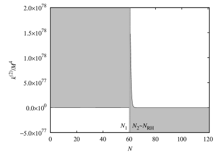
Figure 8: The regions satisfying the constraint (II) for $\tilde{k}^{(2)}(N)$ of model 2.

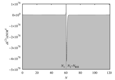
Figure 9: The regions satisfying the constraint (34) for $\tilde{k}^{(2)\prime}(N)$ of model 2.

III.3 The dynamics of the scalar field

The evolution of the expansion in universe does not change even if we consider the model with $\tilde{K}^{(n)}=0$ $(n\geq 2)$, which corresponds to the usual inflaton and/or quintessence models since the time evolution of the system is controlled only by $\tilde{K}^{(0)}(\phi)$ and $\tilde{K}^{(1)}(\phi)$. In case of $\tilde{K}^{(n)}=0$ $(n\geq 2)$, the scalar field becomes canonical and the dynamics of the scalar field is compared with the dynamics of a classical particle in a potential. In case of $\tilde{K}^{(n)}=0$ $(n\geq 2)$, in order to generate the development of the universe expansion given by in the previous Subsections III.1 and III.2, the potential has typically the form depicted in FIG. 10.

Figure 10: The effective potential of the canonical scalar field.

As an initial condition, the scalar field should almost stay near the top of the potential in order to generates the inflation. After that, it rolls down to the bottom of the potential and creates the particles. Finally, without getting trapped in the bottom of the potential, the scalar field goes through the subsequent small peak of the potential and plays the roll of the dark energy.

It is important that different from the inflaton or quintessence models, we need not to fine-tune the initial conditions for the scalar field and there are no tachyonic instability in the models we have constructed even if the effective potential is concave downwards since the motion of the scalar field can be stabilized by their $\tilde{K}^{(2)}(\phi)$ term which should not vanish.

IV A mechanism of the particle production

Now we assume the Hubble rate is given in terms of the e-folding $N$ as $H=H(N)$ and consider the situation that the e-folding $N$ can be identified with a scalar field $\phi$. We now consider the interaction between the scalar field $\phi$ between another real scalar field $\varphi$ as follows,

$$H_{\mathrm{int}}=-\frac{C_{0}}{2}\int d^{3}x\sqrt{-g}\frac{d\rho_{\phi}(\phi)}{d\phi}\varphi^{2}\,.$$ (50)

Here $C_{0}$ is a constant. Note that $\rho_{\phi}(\phi)$ is not the real energy density of $\phi$ but merely a function of $\phi$ given by replacing $N$ in $\rho_{\phi}(N)$ in (35) by $\phi$. We assume that $\phi$ can be treated as an external source and the interaction occurs only in a narrow region around $t=0$ and we approximate $C_{0}\frac{d\rho_{\phi}(\phi)}{d\phi}$ as a function of the cosmological time $t$. We now approximate $C_{0}\frac{d\rho_{\phi}(\phi)}{d\phi}$ by the Gauss function:

$$-C_{0}\frac{d\rho_{\phi}(\phi)}{d\phi}=\frac{U_{0}}{\Delta\sqrt{\pi}}\mathrm{e}^{-\frac{t^{2}}{\Delta^{2}}}\,.$$ (51)

Here $U_{0}$ is a constant and $\Delta$ is the standard deviation. We also assume that the space-time can be regarded as static and also flat when $\left|t\right|\sim\Delta$, which should be checked.

Then the amplitude that the vacuum could transit to two-particle state whose momenta are given by $\bm{p}$ and $\bm{q}$ is given by

$$A_{\bm{p}\bm{q}} = i\int_{-\infty}^{\infty}dt\left<\bm{p},\bm{q}\left|H_{\mathrm{int}}\right|0\right>$$ (52)

$$= i\frac{U_{0}}{\Delta\sqrt{\pi}}\int_{-\infty}^{\infty}dt\int d^{3}x\frac{\mathrm{e}^{-\frac{t^{2}}{\Delta^{2}}-i\left(\omega_{p}+\omega_{q}\right)+i\left(\bm{p}+\bm{q}\right)\cdot\bm{x}}}{2\sqrt{\omega_{p}\omega_{q}}}$$

$$= i\delta^{3}\left(\bm{p}+\bm{q}\right)\frac{U_{0}\mathrm{e}^{-\Delta^{2}\omega_{p}^{2}}}{2\omega_{p}}\,.$$

Here $\omega_{p}=\sqrt{\bm{p}^{2}+m_{\varphi}^{2}}$ with the mass $m_{\varphi}$ of $\varphi$. Then the transition probability is given by

$$P_{2}=\frac{1}{2}\int d^{3}p\,d^{3}q\,\delta^{3}\left(\bm{p}+\bm{q}\right)^{2}\frac{U_{0}^{2}\mathrm{e}^{-2\Delta^{2}\omega_{p}^{2}}}{4\omega_{p}^{2}}\\ =\frac{VU_{0}^{2}}{16\pi^{2}}\int p^{2}dp\frac{\mathrm{e}^{-2\Delta^{2}\omega_{p}^{2}}}{\omega_{p}^{2}}\,.$$

The factor $1/2$ in the first line appears since $\left<\bm{p},\bm{q}\right|=\left<\bm{q},\bm{p}\right|$ and $V$ is the volume of space which appears since

$$\delta^{3}(0)=\frac{V}{\left(2\pi\right)^{3}}\,.$$ (53)

Especially when $\varphi$ is massless, that is, $m_{\varphi}=0$, we find

$$P_{2}=\frac{VU_{0}^{2}}{8\left(2\pi\right)^{\frac{3}{2}}\Delta}\,,$$ (54)

which diverges when $\Delta\to 0$.

Then the total transition probability per unit volume is given by

$$p_{2}=\frac{P_{2}}{V}\,.$$ (55)

Therefore the particle density $n$ is given by

$$n=2p_{2}\,.$$ (56)

We now consider about the energy (density). Eq. (52) tells that the expectation value of the energy $E_{2}$ corresponding to two particles state is given by

$$E_{2}=\frac{1}{2}\int d^{3}p\,d^{3}q\,\delta^{3}\left(\bm{p}+\bm{q}\right)^{2}\frac{2\omega_{p}U_{0}^{2}\mathrm{e}^{-2\Delta^{2}\omega_{p}^{2}}}{4\omega_{p}^{2}}\\ =\frac{VU_{0}^{2}}{8\pi^{2}}\int p^{2}dp\frac{\mathrm{e}^{-2\Delta^{2}\omega_{p}^{2}}}{\omega_{p}}\,.$$

Especially when $\varphi$ is massless, we find

$$E_{2}=\frac{VU_{0}^{2}}{8\left(2\pi\right)^{\frac{3}{2}}\Delta}\,.$$ (57)

Then the expectation value of the energy density $\epsilon_{2}$ for the two particle state is given by

$$\epsilon_{2}=\frac{E_{2}}{V}\,.$$ (58)

We may estimate the width $\Delta$ in (51) by using $N_{1}$ and $N_{2}$ in (37) as

$$\Delta N=N_{2}-N_{1}=\int H\,dt\simeq H_{\mathrm{I}}\int dt=2H_{\mathrm{I}}\Delta\,,$$ (59)

which gives $\Delta N\simeq 2.98\Delta_{1}$ for model 1 and $\Delta N\simeq 4.34\Delta_{2}$ for model 2. Then since the energy density of the radiation in the present universe is given by the product of the critical density $\rho_{\mathrm{cr}0}$ and the density parameter $\Omega_{\mathrm{r}0}$ for the radiation. Since

$$\rho_{\mathrm{cr}0}=10^{-47}\,\mathrm{GeV}^{4}\,,\quad\Omega_{\mathrm{r}0}=8.4\times 10^{-5}\,,$$ (60)

we find

$$\epsilon_{2}=\Omega_{\mathrm{r}0}\rho_{\mathrm{cr}0}\left(\frac{T_{\mathrm{RH}}}{T_{0}}\right)^{4}=10.4\times 10^{-10}\mbox{--}10^{54}\,\mathrm{GeV}^{4}\simeq\frac{4\times 10^{22}\,\mathrm{GeV}^{2}U_{0}^{2}}{8(2\pi)^{3/2}\Delta N^{2}}\,,$$ (61)

which tells

$$U_{0}=9.86\Delta_{1}\times 10^{-15}\mbox{--}10^{17}\,\mathrm{GeV}\quad\mbox{for model 1}\,,\quad 1.43\Delta_{2}\times 10^{-14}\mbox{--}10^{18}\,\mathrm{GeV}\quad\mbox{for model 2}\,.$$ (62)

In (61), $T_{0}$ is the temperature of the present universe.

V Summary

In this paper, after reviewing the formulation of reconstruction for $k$-essence, we explicitly constructed two models which unify the inflation in the early universe and the late-time acceleration in the present universe, and satisfy the observational constraints. We have proposed a mechanism of the interaction for particle production by the quantum effects coming from the variation of the energy density of the scalar field and estimated the energy density of the particles.

In both of the models, the solutions describing the development of the universe expansion are stabilized by $\tilde{K}^{(2)}$ or $\tilde{k}^{(2)}$ terms which should not vanish. We also note that $\tilde{K}^{(2)}$ or $\tilde{k}^{(2)}$ terms play the role to eliminate the tachyon. As explained in Subsection III.3, the solutions describing the development of the expansion in our models can be realized by the usual inflaton or quintessence model, where the scalar field is canonical, but in the canonical scalar models, the solutions could be often unstable and there could appear a tachyon when the scalar field lies at the concave part of the potential. The instability of the canonical scalar models require the fine tuning of the initial conditions, which makes the models unnatural. In our models, due to the stability of the solutions controlled by the $\tilde{K}^{(2)}$ or $\tilde{k}^{(2)}$ terms, there could exist a wide region of the possible initial conditions. Then in the framework given in this paper, we can construct a model describing the time development, which cannot be realized by a usual inflaton or quintessence model.

The roles of $\tilde{K}^{(n)}$ ($n\geq 3$) are, however, still unclear although these terms play the role to guarantee the existence of the Schwarzschild solution Nojiri:2009fq ; Nojiri:2010wj . More detailed cosmological constraints may restrict the form of these terms. It might be interesting to consider the reconstruction of the general spherical symmetric solution in the $k$-essence model as in Nojiri:2006jy .

References

(1)
D. N. Spergel et al. [ WMAP Collaboration ],
Astrophys. J. Suppl. 148, 175-194 (2003).
[astro-ph/0302209];
H. V. Peiris et al. [ WMAP Collaboration ],
Astrophys. J. Suppl. 148, 213 (2003).
[astro-ph/0302225];
D. N. Spergel et al. [ WMAP Collaboration ],
Astrophys. J. Suppl. 170, 377 (2007).
[astro-ph/0603449].
(2)
E. Komatsu et al. [ WMAP Collaboration ],
Astrophys. J. Suppl. 180, 330-376 (2009).
[arXiv:0803.0547 [astro-ph]].
(3)
S. Perlmutter et al. [ Supernova Cosmology Project Collaboration ],
Astrophys. J. 517, 565-586 (1999).
[astro-ph/9812133];
A. G. Riess et al. [ Supernova Search Team Collaboration ],
Astron. J. 116, 1009-1038 (1998).
[astro-ph/9805201];
A. G. Riess, L. -G. Strolger, S. Casertano, H. C. Ferguson, B. Mobasher, B. Gold, P. J. Challis, A. V. Filippenko et al.,
Astrophys. J. 659, 98-121 (2007).
[astro-ph/0611572].
(4)
P. Astier et al. [ The SNLS Collaboration ],
Astron. Astrophys. 447, 31-48 (2006).
[astro-ph/0510447].
(5)
T. Chiba, T. Okabe and M. Yamaguchi,
Phys. Rev. D 62, 023511 (2000)
[arXiv:astro-ph/9912463].
(6)
C. Armendariz-Picon, V. F. Mukhanov and P. J. Steinhardt,
Phys. Rev. Lett. 85, 4438 (2000)
[arXiv:astro-ph/0004134].
(7)
C. Armendariz-Picon, V. F. Mukhanov and P. J. Steinhardt,
Phys. Rev. D 63, 103510 (2001)
[arXiv:astro-ph/0006373].
(8)
C. Armendariz-Picon, T. Damour and V. F. Mukhanov,
Phys. Lett. B 458, 209 (1999)
[arXiv:hep-th/9904075].
(9)
J. Garriga and V. F. Mukhanov,
Phys. Lett. B 458, 219 (1999)
[arXiv:hep-th/9904176].
(10)
A. Sen,
JHEP 0204, 048 (2002)
[arXiv:hep-th/0203211].
(11)
A. Sen,
Mod. Phys. Lett. A 17, 1797 (2002)
[arXiv:hep-th/0204143].
(12)
G. W. Gibbons,
Phys. Lett. B 537, 1 (2002)
[arXiv:hep-th/0204008].
(13)
J. S. Bagla, H. K. Jassal and T. Padmanabhan,
Phys. Rev. D 67, 063504 (2003)
[arXiv:astro-ph/0212198].
(14)
N. Arkani-Hamed, H. C. Cheng, M. A. Luty and S. Mukohyama,
JHEP 0405, 074 (2004)
[arXiv:hep-th/0312099].
(15)
N. Arkani-Hamed, P. Creminelli, S. Mukohyama and M. Zaldarriaga,
JCAP 0404, 001 (2004)
[arXiv:hep-th/0312100].
(16)
P. J. E. Peebles and B. Ratra,
Astrophys. J. 325, L17 (1988).
(17)
B. Ratra and P. J. E. Peebles,
Phys. Rev. D 37, 3406 (1988).
(18)
T. Chiba, N. Sugiyama and T. Nakamura,
Mon. Not. Roy. Astron. Soc. 289, L5 (1997)
[arXiv:astro-ph/9704199].
(19)
I. Zlatev, L. M. Wang and P. J. Steinhardt,
Phys. Rev. Lett. 82, 896 (1999)
[arXiv:astro-ph/9807002].
(20)
S. Nojiri and S. D. Odintsov,
J. Phys. Conf. Ser. 66, 012005 (2007)
[arXiv:hep-th/0611071].
(21)
E. Elizalde, S. ’i. Nojiri, S. D. Odintsov, D. Saez-Gomez, V. Faraoni,
Phys. Rev. D77, 106005 (2008).
[arXiv:0803.1311 [hep-th]].
(22)
S. Nojiri,
Mod. Phys. Lett. A 25, 859 (2010)
[arXiv:0912.5066 [hep-th]].
(23)
S. ’i. Nojiri, S. D. Odintsov, D. Saez-Gomez,
Phys. Lett. B681, 74-80 (2009).
[arXiv:0908.1269 [hep-th]].
(24)
J. Matsumoto and S. Nojiri,
Phys. Lett. B 687, 236 (2010)
[arXiv:1001.0220 [hep-th]].
(25)
S. Nojiri and S. D. Odintsov,
arXiv:1011.0544 [gr-qc].
(26)
S. Nojiri and S. D. Odintsov,
Gen. Rel. Grav. 38, 1285 (2006)
[arXiv:hep-th/0506212].
(27)
S. Capozziello, S. Nojiri and S. D. Odintsov,
Phys. Lett. B 632, 597 (2006)
[arXiv:hep-th/0507182].
(28)
S. ’i. Nojiri, S. D. Odintsov, H. Stefancic,
Phys. Rev. D74, 086009 (2006).
[hep-th/0608168].