FMR and voltage induced transport in normal metal$-$ferromagnet$-$superconductor trilayers

Abstract

We study the subgap spin and charge transport in normal metal-ferromagnet-superconductor trilayers induced by bias voltage and/or magnetization precession. Transport properties are discussed in terms of time-dependent scattering theory. We assume the superconducting gap is small on the energy scales set by the Fermi energy and the ferromagnetic exchange splitting, and compute the non-equilibrium charge and spin current response to first order in precession frequency, in the presence of a finite applied voltage. We find that the voltage-induced instantaneous charge current and longitudinal spin current are unaffected by the precessing magnetization, while the pumped transverse spin current is determined by spin-dependent conductances and details of the electron-hole scattering matrix. A simplified expression for the transverse spin current is derived for structures where the ferromagnet is longer than the transverse spin coherence length.

I Introduction

Experimental and theoretical studies of spin polarized transport in hybrid magnetic nanostructures is a frontier in mesoscopic physics. The most prominent example of conceptual, technological, and commercial impact is the giant magnetoresistance effect utilized in magnetic information storage devices. In order to gain a deeper understanding of spin and charge transport, and to enhance circuit functionality and efficiency, more complex structures are fabricated and studied. In recent years, hybrid nanoscale circuits containing normal conductors, ferromagnets, and superconductors have been realized. These structures allow observation and understanding of competing mechanisms of electron-electron interactions.

The simultaneous existence of ferromagnetism and superconductivity is rare. In ferromagnets, the exchange interaction lifts the spin-degeneracy and induces an itinerant spin polarization. In s-wave superconductors, on the other hand, electrons with anti-parallel spins form Cooper pairs. In homogenous conventional ferromagnets (Fe, Ni, Co, and alloys thereof), the large exchange interaction efficiently dephases electron-hole pairs, and eliminates singlet superconducting correlations over distances larger than the ferromagnetic coherence length. This would suggest a short-range superconducting proximity effect in transition metal ferromagnets.Kawaguchi and Sohma (1992); Demler et al. (1997) Such a simple picture cannot explain recent measurements on Co and Ni ferromagnets coupled to Al superconductors, however, where a substantial resistance drop was observed at the onset of superconductivity.Giroud et al. (1998); Petrashov et al. (1999) The simple picture also fails to explain the long-range superconducting proximity effect recently observed via the Josephson supercurrent through a half-metallic ferromagnet.Keizer et al. (2006); Anwar et al. (2006) Subsequent theoretical work show that induced triplet superconducting correlations give rise to long ranged proximity effect in transition metal ferromagnets.Bergeret et al. (2001); Kadigrobov et al. (2001) Triplet superconducting correlations are insensitive to the pair-breaking exchange interaction and exhibit a longer coherence length, similar to that of superconducting correlations in normal metals. It is now established that spin-flip processes in a ferromagnet can convert singlet into triplet pair correlations. A spatially inhomogeneous magnetization texture Bergeret et al. (2005) or magnons Tkachov et al. (2001); Takahashi et al. (2007); Houzet (2008) are examples of spin-flip sources that are able to induce long ranged triplet correlations.

In this report, we focus our attention on the influence of magnons on the transport properties in normal metal-ferromagnet-superconductor systems. Even normal metal-ferromagnet systems without superconductors exhibit intriguing physics, and especially the interaction between spin and charge currents and the magnetic order parameter in such structures have attracted tremendous interest. For instance, a non-collinear spin flow towards a ferromagnet exerts a torque on the magnetization, a spin transfer torque, that can excite the magnetization and even induce steady state, precessional motion of the ferromagnetic order parameter.Slonczewski (1996); Berger (1996) The inverse effect is also of significant interest: A precessing ferromagnet in electrochemical equilibrium with its environment, acts as a “spin battery” by emitting (or “pumping”) pure spin currents into neighboring materials.Tserkovnyak et al. (2005) When emitted spins are dissipated in adjacent materials, spin pumping enhances magnetic dissipation in the precessing ferromagnet, and thus increases observed linewidths in FMR experiments.Mizukami et al. (2001)

Some ideas from spin transfer physics in normal metal-ferromagnet structures were recently used to study superconductor-ferromagnet systems. A FMR experimentBell et al. (2008) and the following theoretical analysisMorten et al. (2008) have shown how spin pumping can be used to visualize proximity effects and spin relaxation processes inside the superconductor. In essence, in metallic contacts, ferromagnetic correlations reduce the superconducting order parameter close to the layer interface, enabling pumped sub-gap electrons to enter and deposit spin in the superconductor. This is a prime example of how the inverse proximity effect affects the FMR linewidth broadening when typical spin-flip lengths are comparable to the superconducting coherence length.Sillanpää et al. (2001)

We direct our attention to a different aspect of the interplay between magnetization and carrier dynamics in ferromagnet-superconductor structures. In contrast to the works mentioned above, where the magnetization dynamics have been the primary concern, we will consider how a precessing magnetization and an applied voltage bias induce spin and charge currents in a normal metal-ferromagnet-superconductor (N—F—S) trilayer. The computed charge currents can be measured directly, whereas spin currents can possibly be measured by its dissipative effect on the precessing ferromagnet, its spin transfer torque effect on a second ferromagnet, or via spin-filtering as a charge buildup on another ferromagnet.Tserkovnyak et al. (2005) Related to our work, sub-gap transport properties have recently been studied in a normal metal-ferromagnetic superconductor structure.Brataas and Tserkovnyak (2004) In ferromagnetic superconductors, magnetic and electron-hole correlations coexist which can result in novel transport and dynamical magnetic phenomena. It was shown how superconducting correlations, namely Andreev reflections at the layer interface, add features to the results of spin and charge pumping in normal metal-ferromagnet systems. In this report, we also consider how pumping in the N—F—S trilayer is related to pumping in the normal metal-ferromagnetic superconductor system as studied in Ref. Brataas and Tserkovnyak, 2004.

Diffusive transport in hybrid superconductor-normal metal systems is usually formulated within a quasiclassical description.Rammer and Smith (1986) Although this description give qualitative insight into transport properties of superconductor-ferromagnet systems,Bergeret et al. (2005); Houzet (2008) the formalism is limited to ferromagnets with exchange interactions much smaller than the Fermi energy. Thus, a quasiclassical description cannot be used to quantitatively study transport in transition metal ferromagnets Fe, Ni and Co used in experiments. This is one of the reaons why we adopt the scattering theory to transport.Büttiker (1992) Another reasone is that scattering theory captures adiabatic slow time-dependent variations of the magnetization direction well.

Scattering theory has proven most useful in the study of stationary charge and spin currents in magnetoelectronic structures,Brataas et al. (2006) and the time-dependent generalization has successfully been applied to describe parametric pumping of chargeBüttiker et al. (1994); Brouwer (1998); Büttiker and Moskalets (2006) and spin currents.Tserkovnyak et al. (2005) For the N—F—S structure under consideration, we derive charge- and spin currents in the normal metal conductor in response to a slowly precessing ferromagnetic exchange field and applied bias voltage. We focus on sub-gap energies, and how Andreev scattering contributes to the conductivites of the currents. In electro-chemical equilibrium, we make contact with the results for pumping in normal metal-ferromagnetic superconductor structures.Brataas and Tserkovnyak (2004) We proceed by detailing how time- and energy gradients of the total scattering matrix contribute to non-equilibrium pumped currents, and find that both charge and longitudinal spin currents are unaffected by the precessing magnetization. Finally, we consider non-equilibrium charge and spin currents for trilayers where the ferromagnetic region is longer than the transverse spin coherence length.

This paper is organized in the following way: The N—F—S system is described in Sec. II. In Sec. III, we use time-dependent scattering theory to derive general expressions for charge and spin currents to first order in pumping frequency. The total scattering matrix for the system is then invoked in Sec. IV to obtain non-equilibrium pumped currents. Our conclusions are in Sec. V.

II Model description

The system is sketched in Fig. 1. It consists of a superconductor (S) in series with a ferromagnet (F) and a normal metal lead (N₁). N₁ is ideally coupled to a normal metal reservoir (N${}_{\text{res}}$). We assume N${}_{\text{res}}$ and S to be in local thermal equilibrium, and denote a possible chemical potential difference between the normal and the superconducting side as $\mu_{N}-\mu_{S}=eV$. Spin-orbit interactions are disregarded, and the ferromagnetic order parameter is assumed to be homogeneous and with a fixed magnitude $\Delta_{xc}$ inside F. Its direction is along the time-dependent unit vector $\boldsymbol{m}(t)=(\sin\theta(t)\cos\Omega t,\sin\theta(t)\sin\Omega t,\cos\theta(t))$. The precessing magnetization serves as the pumping parameter in the system.

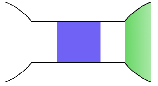
Figure 1: A ferromagnetic scattering region (F) is connected to a superconductor (S) and a normal metal reservoir (N${}_{\text{res}}$) via two normal metal leads (N₁ and N₂). Amplitudes of outgoing (incoming) carrier states are given by $b$ ($a$).

We focus on sub-gap transport properties. Thus, possible scattering processes include Andreev reflections at the F—S interfaceAndreev (1964) and spin-dependent normal scattering inside F. Following a standard procedure,Beenakker (1992) the scattering problem is greatly simplified by utilizing spatially separated regions where scattering processes occur. This is achieved by inserting a fictitious normal metal lead (N₂) between F and S. We assume that N₂ is longer than the Fermi wavelength, so that asymptotic, plane wave solutions are applicable in this region. The total scattering matrix is a concatenation of the scattering matrices for N₁—F—N₂ and for Andreev reflections at the N₂—S interface. Transport between F and S is mediated by the ballistic N₂ lead.

The singlet superconductor is described by the BCS Hamiltonian

$$\hat{\mathcal{H}}=\sum_{\sigma=\uparrow,\downarrow}\int\mathrm{d}\boldsymbol{r}\>\hat{\Psi}^{\dagger}_{\sigma}(\boldsymbol{r})H_{0}(\boldsymbol{r})\hat{\Psi}_{\sigma}(\boldsymbol{r})\\ +\int\mathrm{d}\boldsymbol{r}\>\left\{\Delta(\boldsymbol{r})\hat{\Psi}^{\dagger}_{\uparrow}(\boldsymbol{r})\hat{\Psi}^{\dagger}_{\downarrow}(\boldsymbol{r})+\Delta^{*}(\boldsymbol{r})\hat{\Psi}_{\downarrow}(\boldsymbol{r})\hat{\Psi}_{\uparrow}(\boldsymbol{r})\right\},$$ (1)

where $H_{0}$ is the normal state, single-particle Hamiltonian and $\Delta(\boldsymbol{r})$ the superconducting gap. We model the gap by a step function, $\Delta(\boldsymbol{r})=\Delta\mathrm{e}^{\mathrm{i}\phi}\Theta(x)$, where the phase $\phi$ is constant, and $x$ is the coordinate perpendicular to the N₂—S interface. We take the Fermi energy $E_{F}$ to be the largest energy scale, and focus on the low energy transport properties in regimes when the superconducting gap is much less than the exchange interaction in the ferromagnet $\Delta_{xc}$, $eV\leq\Delta\ll\Delta_{xc},E_{F}$. The Hamiltonian (1) is diagonalized by the following Bogoliubov transformationKetterson and Song (1999)

$$\hat{\Psi}_{\sigma}(\boldsymbol{r})=\sum_{n}\left\{\hat{\gamma}_{n}u_{n}(\boldsymbol{r},\sigma)+\hat{\gamma}^{\dagger}_{n}v^{*}_{n}(\boldsymbol{r},\sigma)\right\},$$ (2)

where $\hat{\gamma}_{n}^{(\dagger)}$ are quasiparticle annihilation (creation) operators that satisfy the fermionic anti-commutation relation

$$\{\hat{\gamma}_{m},\hat{\gamma}^{\dagger}_{n}\}=\delta_{m,n}.$$ (3)

The transformation (2) results in a matrix equation for the quasiparticle eigenfunctions $u_{n}$ and $v_{n}$:

$$\begin{pmatrix}H_{0}(\boldsymbol{r})&\mathrm{i}\Delta(\boldsymbol{r})\sigma^{y}\\ -\mathrm{i}\Delta^{*}(\boldsymbol{r})\sigma^{y}&-H_{0}^{*}(\boldsymbol{r})\end{pmatrix}\begin{pmatrix}u_{n}(\boldsymbol{r})\\ v_{n}(\boldsymbol{r})\end{pmatrix}=\varepsilon_{n}\begin{pmatrix}u_{n}(\boldsymbol{r})\\ v_{n}(\boldsymbol{r})\end{pmatrix}.$$ (4)

The quasiparticle excitation energy $\varepsilon_{n}$ is measured with respect to the chemical potential of the superconductor, which is set to zero. $\sigma^{y}$ is a Pauli matrix operating in spin space. The Bogoliubov-de Gennes Hamiltonian (4) is the starting point when we in Sec. III.2 derive the appropriate reflection amplitudes for quasiparticles impinging on the superconductor interface.

III Time-dependent scattering theory

We now focus on the time-dependent scattering theory for the N—F—S structure in Fig. 1, apply the general framework established in Refs. Büttiker et al., 1994; Brouwer, 1998; Vavilov et al., 2001; Tserkovnyak et al., 2005; Büttiker and Moskalets, 2006, and make use of the scattering theory for hybrid superconductor-normal metal structures discussed in Refs. Beenakker, 1992; Blaauboer, 2002. We find it most convenient to study a slowly precessing magnetization by a scattering matrix expressed in the Wigner representation,Rammer and Smith (1986) making the derivation of pumped currents similar to that carried out for normal systems in Refs. Wang and Wang, 2002a, b.

In order to describe a scattering potential of arbitrary time-dependence, we start by considering the two-time scattering matrix $\mathcal{S}(t,t^{\prime})$, that relates annihilation operators between states outgoing and incoming from the scattering region:

$$\hat{b}_{\alpha}(t)=\sum_{\beta}\int\mathrm{d}t^{\prime}\mathcal{S}_{\alpha\beta}(t,t^{\prime})\hat{a}_{\beta}(t^{\prime}).$$ (5)

As indicated in Fig. 1, $\hat{b}_{\alpha}:(\hat{a}_{\alpha})$ annihilates the outgoing (incoming) state $\alpha$. $\alpha$ labels electron-hole Nambu space index, spin and transverse wave-guide number. We assume that the reservoirs connected to the scattering region are in local thermal equilibrium, and that incoming carriers from the normal metal reservoir fulfill

$$\langle\hat{a}_{\alpha}^{\dagger}(\varepsilon)\hat{a}_{\alpha^{\prime}}(\varepsilon^{\prime})\rangle=\delta_{\alpha,\alpha^{\prime}}\delta(\varepsilon-\varepsilon^{\prime})f_{\alpha}(\varepsilon),$$ (6)

where the brackets indicate a quantum and statistical average, and

$$f_{e(h)}(\varepsilon)=f_{0}(\varepsilon-\sigma^{e(h)}eV)\\ =\left[1+\mathrm{e}^{(\varepsilon-\sigma^{e(h)}eV)/k_{B}T_{el}}\right]^{-1},$$ (7)

where $\sigma^{e(h)}=+(-)1$, and $f_{e(h)}(\varepsilon)$ is the Fermi-Dirac distribution of incoming electrons (holes) at a charge bias $eV$ and electron temperature $T_{el}$. We will eventually consider electron temperature to be lower than the superconducting gap. the We will now proceed by computing charge and spin currents in the system.

III.1 Matrix current

We seek the right-going charge and spin currents in normal metal lead 1, and start by introducing the matrix currentTserkovnyak and Brataas (2001)

$$\hat{I}_{1,\alpha\beta}(t)=2\pi e\tau^{z}_{\alpha\beta}\left(\hat{a}^{\dagger}_{\beta}(t)\hat{a}_{\alpha}(t)-\hat{b}^{\dagger}_{\beta}(t)\hat{b}_{\alpha}(t)\right),$$ (8)

where $e$ is the electronic charge, and $\tau^{z}$ is a Pauli matrix in electron-hole space:

$$\tau^{z}=\begin{pmatrix}1&0\\ 0&-1\end{pmatrix}.$$ (9)

Charge and spin currents are obtained from the matrix current (8) as follows:

$$I_{c}(t)=\sum_{\alpha}\langle\hat{I}_{1,\alpha\alpha}(t)\rangle,$$ (10)

and

$$\boldsymbol{I}_{s}(t)=\frac{1}{2e}\sum_{\alpha,\beta}\boldsymbol{\rho}_{\alpha\beta}\langle\hat{I}_{1,\beta\alpha}(t)\rangle,$$ (11)

respectively. Summations run over electron-hole, spin and mode space, and $\boldsymbol{\rho}$ is a matrix with diagonal structure in electron-hole space:

$$\boldsymbol{\rho}_{\alpha\beta}\equiv\begin{pmatrix}\boldsymbol{\sigma}_{\alpha\beta}&0\\ 0&\boldsymbol{\sigma}^{*}_{\alpha\beta}\end{pmatrix},$$ (12)

and with a vector of the Pauli matrices and their complex conjugates, as the diagonal elements.

For a slowly oscillating scatterer, it is convenient to express the scattering matrix in the Wigner representationRammer and Smith (1986); Wang and Wang (2002a, b)

$$\mathcal{S}_{\alpha\beta}(t,t^{\prime})=\int_{0}^{\infty}\frac{\mathrm{d}\varepsilon}{2\pi}\mathrm{e}^{-\mathrm{i}\varepsilon(t-t^{\prime})}\mathcal{S}_{\alpha\beta}\left(\varepsilon;\frac{t+t^{\prime}}{2}\right).$$ (13)

In this representation, the matrix current is:

$$\langle\hat{I}_{1,\alpha\beta}(t)\rangle=\frac{e}{2\pi}\tau^{z}_{\alpha\beta}\biggr{\{}\delta_{\alpha,\beta}\int_{0}^{\infty}\mathrm{d}\varepsilon\>f_{\alpha}(\varepsilon)-\sum_{\gamma}\int_{-\infty}^{\infty}\mathrm{d}\tau\>\mathrm{d}T\int_{0}^{\infty}\frac{\mathrm{d}\varepsilon_{1}\>\mathrm{d}\varepsilon_{2}}{2\pi}f_{\gamma}(\tau)\\ \times\mathrm{e}^{-\mathrm{i}\varepsilon_{1}(T-\tau/2)}\mathrm{e}^{\mathrm{i}\varepsilon_{2}(T+\tau/2)}\mathcal{S}_{\alpha\gamma}\left(\varepsilon_{2};t+\frac{T+\tau/2}{2}\right)\mathcal{S}^{*}_{\beta\gamma}\left(\varepsilon_{1};t+\frac{T-\tau/2}{2}\right)\biggr{\}}.$$ (14)

The current is expressed in terms of the center and relative time coordinates $T=(t^{\prime}+t^{\prime\prime})/2$ and $\tau=t^{\prime\prime}-t^{\prime}$, and the Fourier transform of the distribution function

$$f_{\gamma}(\tau)\equiv\int_{0}^{\infty}\frac{\mathrm{d}\varepsilon}{2\pi}\mathrm{e}^{-\mathrm{i}\varepsilon\tau}f_{\gamma}(\varepsilon).$$ (15)

When the scattering matrix $\mathcal{S}(\varepsilon;t)$ is a concatenation of multiple time-dependent scattering elements, the Wigner representation of $\mathcal{S}$ will also be an infinite sum of time and energy gradients.Rammer and Smith (1986) The magnetization dynamics is slow as compared to the time an electron spends in the scattering region. In the adiabatic approximation, we assume the scattering matrix evolves on a much longer timescale than the typical dwell times of particles inside the scattering region. In this regime, we formally expand $\mathcal{S}$ asMoskalets and Büttiker (2004)

$$\mathcal{S}(\varepsilon;t)=S_{0}(\varepsilon;t)+A(\varepsilon;t)+\mathcal{O}(\partial_{t}^{2}S_{0})$$ (16)

where $S_{0}$ is the “frozen” or instantaneous scattering matrix, and the matrix $A$ represents all first-order gradient corrections to $S_{0}$ resulting from the concatenation of time-dependent scattering elements that describe the device. Unitarity of $\mathcal{S}$ to all orders in time- and energy-gradients impliesMoskalets and Büttiker (2004)

$$S_{0}A^{\dagger}+AS_{0}^{\dagger}=\frac{\mathrm{i}}{2}\left(\partial_{t}S_{0}\partial_{\varepsilon}S_{0}^{\dagger}-\partial_{\varepsilon}S_{0}\partial_{t}S_{0}^{\dagger}\right)\equiv\frac{1}{2}P\left\{S_{0};S_{0}^{\dagger}\right\},$$ (17)

where a Poisson bracket $P\{.;.\}$ has been defined to ease the notation. In the following, scattering matrix arguments $(\varepsilon;t)$ are omitted in places where there is no risk of confusion.

To obtain a local (in time) expression for the matrix current (14), we Taylor expand $\mathcal{S}$ to first order in time derivatives, and obtain the matrix current

$$\langle\hat{I}_{1,\alpha\beta}(t)\rangle=\frac{e}{2\pi}\tau^{z}_{\alpha\beta}\sum_{\gamma}\int_{0}^{\infty}\mathrm{d}\varepsilon\biggr{\{}\left(f_{\alpha}(\varepsilon)-f_{\gamma}(\varepsilon)\right)\left(S_{0,\alpha\gamma}S_{0,\beta\gamma}^{*}+A_{\alpha\gamma}S^{*}_{0,\beta\gamma}+S_{0,\alpha\gamma}A^{*}_{\beta\gamma}-\frac{1}{2}P\left\{S_{0,\alpha\gamma};S^{*}_{0,\beta\gamma}\right\}\right)\\ +\frac{\mathrm{i}}{2}\left(-\partial_{\varepsilon}f_{\gamma}(\varepsilon)\right)\left(S_{0,\alpha\gamma}\partial_{t}S^{*}_{0,\beta\gamma}-\partial_{t}S_{0,\alpha\gamma}S^{*}_{0,\beta\gamma}\right)\biggr{\}}+\mathcal{O}\left(\partial_{t}^{2}S_{0}\right)$$ (18)

where Eqs. (16) and (17) have been used. The matrix current in Eq. (18) is exact to first order in frequency of the pumping parameter.

Finally, we observe that in the absence of a voltage bias, the gradient corrections to the frozen scattering matrix, represented by $A$, vanish from the matrix current. In electro-chemical equilibrium, when $V=0$, $f_{e}(\varepsilon)=f_{h}(\varepsilon)$, the first line of Eq. (18) vanishes, and the pumped current is determined by the frozen scattering matrix. Naturally, the same is also true for the time-dependent theory based on Floquet scattering matrices.Büttiker and Moskalets (2006)

III.2 Scattering matrix for a N—F—S structure

In this section, the scattering matrix formalism derived for N—S structuresBeenakker (1992) is applied to our N—F—S trilayer. As described in Sec. II, the scattering description of a N—F—S structure is greatly simplified by inserting a fictitious normal metal lead (N₂) between the two scattering regions, thereby spatially separating spin-dependent scattering in F and Andreev reflection at the N₂—S interface.Beenakker (1992) The scattering matrix $S_{F}$, describing the disordered ferromagnetic region, is block-diagonal in electron-hole space. We write $S_{F}$ as

$$S_{F}(\varepsilon;t)=\begin{pmatrix}s_{F}(\varepsilon;t)&0\\ 0&s_{F}(-\varepsilon;t)^{*}\end{pmatrix},$$ (19)

where the diagonal elements are

$$s_{F}=\begin{pmatrix}r_{11}&t_{12}\\ t_{21}&r_{22}\end{pmatrix}.$$ (20)

Here, $r_{ii}$ and $t_{ij}$ are matrices in spin-space that describe reflection of an incoming electron in lead $i$, and transmission of an electron from lead $j$ to lead $i$, respectively.

Electrons and holes with opposite spins are coupled by Andreev reflection at the superconductor interface, where an incoming electron (hole) is reflected as a hole (electron) with reversed spin direction. The reflection amplitudes are derived by matching propagating wave functions in N₂ with evanescent wave functions in the superconductor. The resulting scattering matrix readsBeenakker (1992); Waintal and Brouwer (2002)

$$r^{A}=\begin{pmatrix}0&r^{A}_{eh}\\ r^{A}_{he}&0\end{pmatrix}=\begin{pmatrix}0&\mathrm{i}\alpha\sigma^{y}\mathrm{e}^{\mathrm{i}\phi}\\ -\mathrm{i}\alpha\sigma^{y}\mathrm{e}^{-\mathrm{i}\phi}&0\end{pmatrix},$$ (21)

where $\alpha=\mathrm{exp}\left[-\mathrm{i}\arccos(\varepsilon/\Delta)\right]$.

The total scattering matrix of the N—F—S structure is a concatenation of $S_{F}$ and $r^{A}$, and in terms of the frozen scattering matrices, we obtain the familiar resultsBeenakker (1992); Blaauboer (2002)

$$S_{0}^{ee}(\varepsilon ;t)=r_{11}(\varepsilon)$$

$$+t_{12}(\varepsilon)r^{A}_{eh}(\varepsilon)r^{*}_{22}(-\varepsilon)M_{e}(\varepsilon)r^{A}_{he}(\varepsilon)t_{21}(\varepsilon),$$ (22a)

$$S_{0}^{hh}(\varepsilon ;t)=r_{11}^{*}(-\varepsilon)$$

$$+t^{*}_{12}(-\varepsilon)r^{A}_{he}(\varepsilon)r_{22}(\varepsilon)M_{h}(\varepsilon)r^{A}_{eh}(\varepsilon)t^{*}_{21}(-\varepsilon),$$ (22b)

$$S_{0}^{eh}(\varepsilon ;t)=t_{12}(\varepsilon)M_{h}(\varepsilon)r^{A}_{eh}(\varepsilon)t^{*}_{21}(-\varepsilon),$$ (22c)

$$S_{0}^{he}(\varepsilon ;t)=t^{*}_{12}(-\varepsilon)M_{e}(\varepsilon)r^{A}_{he}(\varepsilon)t_{21}(\varepsilon),$$ (22d)

where time arguments are omitted on the right hand side of the equations for sake of notation. Multiple reflections between S and F, mediated by propagations through N₂, are described by

$$M_{e}(\varepsilon) =\left[1-r^{A}_{he}(\varepsilon)r_{22}(\varepsilon)r^{A}_{eh}(\varepsilon)r^{*}_{22}(-\varepsilon)\right]^{-1},$$ (23)

$$M_{h}(\varepsilon) =\left[1-r^{A}_{eh}(\varepsilon)r^{*}_{22}(-\varepsilon)r^{A}_{he}(\varepsilon)r_{22}(\varepsilon)\right]^{-1}.$$ (24)

From Eqs. (22), and using $r^{A}_{eh}(-\varepsilon)^{*}=r^{A}_{he}(\varepsilon)$, one obtains the following symmetry relations for the total scattering matrix:

$$\mathcal{S}^{ee}(\varepsilon;t)=\left[\mathcal{S}^{hh}(-\varepsilon;t)\right]^{*},$$ (25a)

and

$$\mathcal{S}^{eh}(\varepsilon;t)=\left[\mathcal{S}^{he}(-\varepsilon;t)\right]^{*}.$$ (25b)

The frozen scattering matrices in Eqs. (22) are all time-dependent due to the slowly varying magnetization in the ferromagnet. Arguably the easiest way to evaluate the matrix current, is to perform a spinor rotation that aligns the spin quantization axis with the instantaneous magnetization direction.Tserkovnyak et al. (2005); Brataas and Tserkovnyak (2004) The total scattering matrix

$$S_{0}(\varepsilon;t)=\begin{pmatrix}S_{0}^{ee}&S_{0}^{eh}\\ S_{0}^{he}&S_{0}^{hh}\end{pmatrix}$$ (26)

can be related to the total scattering matrix $\underline{S}$ in the rotating frame by the spinor rotations

$$S_{0}(\varepsilon;t)={W}^{\dagger}(t)\underline{S}(\varepsilon)W(t),$$ (27)

where $W(t)=V(t)U(t)$, with

$$U(t)=\begin{pmatrix}\mathcal{U}(t)&0\\ 0&\mathcal{U}^{\dagger}(t)\end{pmatrix}=\begin{pmatrix}\mathrm{exp}\left[\frac{\mathrm{i}\Omega t}{2}\sigma^{z}\right]&0\\[8.5359pt] 0&\mathrm{exp}\left[-\frac{\mathrm{i}\Omega t}{2}\sigma^{z}\right]\end{pmatrix},$$ (28)

and

$$V(t)=\begin{pmatrix}\mathcal{V}(t)&0\\ 0&\mathcal{V}(t)\end{pmatrix}=\begin{pmatrix}\mathrm{exp}\left[\frac{\mathrm{i}\theta(t)}{2}\sigma^{y}\right]&0\\[8.5359pt] 0&\mathrm{exp}\left[\frac{\mathrm{i}\theta(t)}{2}\sigma^{y}\right]\end{pmatrix}.$$ (29)

In the rotating frame, $\underline{S}_{0}^{ee}$ and $\underline{S}_{0}^{hh}$ are both diagonal in spin space, while $\underline{S}_{0}^{eh}$ and $\underline{S}_{0}^{he}$, which mix spin $\sigma$ electrons with spin $-\sigma$ holes, only have off-diagonal elements.

Now that the matrix current and relevant scattering matrices are derived, we proceed to study pumped charge and spin currents for a voltage biased trilayer structure.

IV Pumped currents out of equilibrium

A complication that arises when the system is driven out of equilibrium, is that time- and energy gradients of the frozen scattering matrix must be evaluated. Before presenting the detailed expressions for charge and spin currents in the normal metal lead, we derive the required gradient corrections. Due to electron-hole symmetry (LABEL:symmetry), it is sufficient to consider only $A^{he}$ in the gradient correction.

IV.1 Gradient correction matrix

In the following, we determine $A^{he}$ by a formal gradient expansion of the corresponding scattering matrix $\mathcal{S}^{he}$, whose full time and energy dependence of $\mathcal{S}^{he}$ is given by (see Eq. (22)):

$$\mathcal{S}^{he}(\varepsilon;t)=\left(t^{*}_{12}\circ M_{e}\circ r^{A}_{he}\circ t_{21}\right)(\varepsilon;t).$$ (30)

Evaluating the convolutions in the Wigner representation can be done by systematically expanding the exponentials:Rammer and Smith (1986)

$$(A\circ B)(\varepsilon;t)=\mathrm{e}^{\mathrm{i}\left(\partial^{A}_{\varepsilon}\partial^{B}_{t}-\partial^{A}_{t}\partial^{B}_{\varepsilon}\right)/2}A(\varepsilon;t)B(\varepsilon;t),$$ (31)

where the superscripts indicate which matrix the operator works on. A significant simplification of the final result is achieved when the superconducting gap is much less than the exchange energy, $\Delta\ll\Delta_{xc},E_{F}$. The energy dependence is then only determined by the energy dependence of the Andreev reflection. Since we are evaluating the energy gradients close to the Fermi level, $\partial_{\varepsilon}s_{F}\ll\partial_{\varepsilon}r^{A}$, and we obtain the simplified expression for the gradient matrix $A^{he}$:

$$A^{he}(\varepsilon;t)\approx-\frac{\mathrm{i}}{2}\partial_{\varepsilon}\partial_{t}S^{he}_{0}+\mathrm{i}t^{*}_{12}\partial_{\varepsilon}(M_{e}r^{A}_{he})\partial_{t}t_{21}\\ +\mathrm{i}t^{*}_{12}\partial_{\varepsilon}\partial_{t}M_{e}r^{A}_{he}t_{21}+\mathrm{i}t^{*}_{12}\partial_{t}M_{e}\partial_{\varepsilon}M_{e}^{-1}M_{e}r^{A}_{he}t_{21}\\ -\mathrm{i}t^{*}_{12}M_{e}r^{A}_{he}\partial_{t}r_{22}\partial_{\varepsilon}r^{A}_{eh}r^{*}_{22}M_{e}r^{A}_{he}t_{21}\\ \equiv-\frac{\mathrm{i}}{2}\partial_{\varepsilon}\partial_{t}S_{0}^{he}+\Gamma^{he}.$$ (32)

Here, $S_{0}^{he}$ is the frozen scattering matrix from Eq. (22), and Before evaluating the currents, we observe that $\Gamma^{he}$ in the rotating frame is diagonal in spin space. This fact, which is important when evaluating non-equilibrium pumped charge and spin currents, can be seen from

$$\Gamma^{he}=\mathcal{U}\mathcal{V}^{\dagger}\underline{\Gamma}^{he}\mathcal{VU},$$ (33)

with

$$\underline{\Gamma}^{he}=\frac{\mathrm{i}}{2}\underline{t}^{*}_{12}\partial_{\varepsilon}(\underline{M}_{e}r^{A}_{he})\Lambda(\underline{t}_{21\uparrow}-\underline{t}_{21\downarrow})\\ +\frac{\mathrm{i}}{2}\underline{t}^{*}_{12}(\underline{M}_{e\uparrow}-\underline{M}_{e\downarrow})\partial_{\varepsilon}(r^{A}_{he}\Lambda\underline{r}_{22}r^{A}_{eh})\underline{r}^{*}_{22}\underline{M}_{e}r^{A}_{he}\underline{t}_{21}\\ -\frac{\mathrm{i}}{2}\underline{t}^{*}_{12}\underline{M}_{e}r^{A}_{he}(\underline{r}_{22\uparrow}-\underline{r}_{22\downarrow})\Lambda\partial_{\varepsilon}r^{A}_{eh}\underline{r}^{*}_{22}\underline{M}_{e}r^{A}_{he}\underline{t}_{21}\\ -\frac{\mathrm{i}}{2}\underline{t}^{*}_{12}\partial_{\varepsilon}(\underline{M}_{e\uparrow}-\underline{M}_{e\downarrow})r^{A}_{he}\Lambda\underline{t}_{21},$$ (34)

where

$$\Lambda\equiv\mathcal{VU}\partial_{t}(\boldsymbol{m}\cdot\boldsymbol{\sigma})\mathcal{U}^{\dagger}\mathcal{V}^{\dagger}=\partial_{t}\theta\sigma^{x}+\sin\theta\Omega\sigma^{y}.$$ (35)

Multiplying $r^{A}_{he}$, which is $\sim\sigma^{y}$, with $\Lambda$, and using that the other components in the equation are all diagonal, brings us to the conclusion that $\underline{\Gamma}^{he}$ is diagonal in spin space. Finally, we note that $\Gamma^{he}\to 0$ for a vanishing ferromagnetic ordering parameter.

Once the gradient corrections to the frozen scattering matrix are derived, one can obtain non-equilibrium pumped currents to first order in pumping frequency.

IV.2 Pumped charge current

According to Eq. (10), the charge current is obtained by tracing the matrix current (18) over electron-hole, spin and mode space. Making use of the electron-hole symmetries from Eqs. (25a)(25b), and using that both $\mathrm{Tr}\left\{\partial_{t}S_{0}^{ee}S_{0}^{ee\dagger}\right\}=0$ and $\mathrm{Tr}\left\{\partial_{t}S_{0}^{he}S_{0}^{he\dagger}\right\}=0$, one finds that the pumped charge current is determined by

$$I_{c}(t)=\frac{e}{2\pi}\int_{-\infty}^{\infty}\mathrm{d}\varepsilon\>\biggr{(}\left[f_{e}(\varepsilon)-f_{h}(\varepsilon)\right]\mathrm{Tr}\Big{\{}S_{0}^{he}S_{0}^{he\dagger}\\ +A^{he}S_{0}^{he\dagger}+S_{0}^{he}A^{he\dagger}-\frac{1}{2}P\left\{S_{0}^{he};S_{0}^{he\dagger}\right\}\Big{\}}\biggr{)},$$ (36)

to first order in pumping parameter frequency. Using that $A^{he}=-\frac{\mathrm{i}}{2}\partial_{\varepsilon}\partial_{t}S_{0}^{he}+\Gamma^{he}$, the current (36) simplifies to

$$I_{c}(t)=\frac{e}{2\pi}\int_{-\infty}^{\infty}\mathrm{d}\varepsilon\>\biggr{(}\left[f_{e}(\varepsilon)-f_{h}(\varepsilon)\right]\\ \times\mathrm{Tr}\Big{\{}S_{0}^{he}S_{0}^{he\dagger}+\Gamma^{he}S_{0}^{he\dagger}+S_{0}^{he}\Gamma^{he\dagger}\Big{\}}\biggr{)}.$$ (37)

Any non-equilibrium pumped contributions to the current are determined by the remainder $\Gamma^{he}$ from Eq. (34). However, as pointed out at the end of Sec. IV.1, $\underline{\Gamma}^{he}$ is a diagonal matrix in spin space. From Eq. (22), we know that $\underline{S}_{0}^{he}$ is strictly off-diagonal in spin space. This implies that $\mathrm{Tr}\left\{\Gamma^{he}S_{0}^{he\dagger}\right\}=0$, and the charge current is reduced to the stationary result:

$$I_{c}=\frac{e}{2\pi}\int_{-\infty}^{\infty}\mathrm{d}\varepsilon\>\left[f_{e}(\varepsilon)-f_{h}(\varepsilon)\right]\tilde{g}(\varepsilon),$$ (38)

where the total conductance is defined as

$$\tilde{g}\equiv\sum_{m,n}\left\{\left|\underline{S}^{he}_{\downarrow\uparrow,mn}\right|^{2}+\left|\underline{S}^{he}_{\uparrow\downarrow,mn}\right|^{2}\right\}.$$ (39)

The result in Eq. (38) shows that there is no pumped charge current in N—F—S structures, even when there is an additional bias voltage driving the system, e.g. there are no bilinear contributions proportional to the bias voltage and the FMR frequency. The stationary result is similar to that obtained in FS—N structures,Brataas and Tserkovnyak (2004) a result that indicates that the total scattering matrix for a disordered region coupled to a ferromagnetic superconductor, is structurally equivalent to that of a disordered ferromagnetic region coupled to a superconductor. The two structures have different scattering matrices, however, and therefore the expressions for the conductances differ.

IV.3 Pumped spin current

We proceed by evaluating the pumped spin current to first order in pumping parameter frequency. Utilizing the electron-hole symmetry relations for the total scattering matrix, we obtain

$$\boldsymbol{I}_{s}(t)=\frac{1}{4\pi}\int_{-\infty}^{\infty}\mathrm{d}\varepsilon\>\left(f_{e}(\varepsilon)-f_{h}(\varepsilon)\right)\left[\mathrm{Tr}\left\{\boldsymbol{\sigma}^{*}\left(S_{0}^{he}S_{0}^{he\dagger}+\Gamma^{he}S_{0}^{he\dagger}+S_{0}^{he}\Gamma^{he\dagger}\right)\right\}+\partial_{\varepsilon}\mathrm{Im}\mathrm{Tr}\left\{\boldsymbol{\sigma}^{*}\partial_{t}S_{0}^{he}S_{0}^{he\dagger}\right\}\right]\\ +\frac{1}{4\pi}\int_{-\infty}^{\infty}\mathrm{d}\varepsilon\>(-\partial_{\varepsilon}f_{e}(\varepsilon))\left[\mathrm{Im}\mathrm{Tr}\left\{\boldsymbol{\sigma}\partial_{t}S_{0}^{ee}S_{0}^{ee\dagger}\right\}-\mathrm{Im}\mathrm{Tr}\left\{\boldsymbol{\sigma}^{*}\partial_{t}S_{0}^{he}S_{0}^{he\dagger}\right\}\right].$$ (40)

Introducing the conductance polarization

$$\tilde{p}\equiv\frac{1}{\tilde{g}}\sum_{m,n}\left\{\left|\underline{S}^{he}_{\downarrow\uparrow,mn}\right|^{2}-\left|\underline{S}^{he}_{\uparrow\downarrow,mn}\right|^{2}\right\},$$ (41)

and the generalized mixing conductanceBrataas and Tserkovnyak (2004)

$$\tilde{g}^{\uparrow\downarrow}\equiv\sum_{m,n}\left\{\delta_{m,n}-\underline{S}^{ee}_{\uparrow,mn}\underline{S}^{ee*}_{\downarrow,mn}+\underline{S}^{he}_{\downarrow\uparrow,mn}\underline{S}^{he*}_{\uparrow\downarrow,mn}\right\}.$$ (42)

we find the following expression for the spin current:

$$\boldsymbol{I}_{s}(t)=-\frac{1}{4\pi}\int_{-\infty}^{\infty}\mathrm{d}\varepsilon\>(f_{e}(\varepsilon)-f_{h}(\varepsilon))\left(\tilde{p}\tilde{g}\boldsymbol{m}(t)-\mathrm{Tr}\left\{\boldsymbol{\sigma}^{*}(\Gamma^{he}S_{0}^{he\dagger}+S_{0}^{he}\Gamma^{he\dagger})\right\}\right)\\ +\frac{1}{8\pi}\int_{-\infty}^{\infty}\mathrm{d}\varepsilon\>(f_{e}(\varepsilon)-f_{h}(\varepsilon))\partial_{\varepsilon}\biggr{(}\boldsymbol{m}\times\partial_{t}\boldsymbol{m}\Big{(}\tilde{g}+2\mathrm{Re}\sum_{m,n}\underline{S}^{he}_{\downarrow\uparrow,mn}\underline{S}^{he*}_{\uparrow\downarrow,mn}\Big{)}+2\partial_{t}\boldsymbol{m}\mathrm{Im}\sum_{m,n}\underline{S}^{he}_{\downarrow\uparrow,mn}\underline{S}^{he*}_{\uparrow\downarrow,mn}\biggr{)}\\ +\frac{1}{4\pi}\int_{-\infty}^{\infty}\mathrm{d}\varepsilon\>\partial_{\varepsilon}f_{e}(\varepsilon)\left(\boldsymbol{m}\times\partial_{t}\boldsymbol{m}\mathrm{Re}\tilde{g}^{\uparrow\downarrow}+\partial_{t}\boldsymbol{m}\mathrm{Im}\tilde{g}^{\uparrow\downarrow}\right).$$ (43)

The term $\sim\tilde{p}\tilde{g}\boldsymbol{m}(t)$ on the right hand side of Eq. (43) corresponds to the non-equilibrium bias voltage spin current observed also in the absence of a precessing magnetization vector. Terms in the final line are similar to those derived previously within electro-chemical equilibrium pumping theory for F—NTserkovnyak et al. (2005), and FS—N structuresBrataas and Tserkovnyak (2004). However, we ask the reader to note that the generalized mixing conductance in Eq. (3) in Ref. Brataas and Tserkovnyak, 2004 is valid for triplet superconductors only; the correct mixing conductance for a singlet superconductor is given by Eq. (42) above. The remaining terms on the right hand side of Eq. (43) are non-equilibrium, pumped contributions to the spin current. They depend on pumping parameter frequency via $\partial_{t}\boldsymbol{m}$ and the $\Lambda$ term from Eq. (35), which is contained in the gradient remainder $\Gamma^{he}$.

Finally, we would like to point out that there are no pumped contributions to the longitudinal spin current $I^{||}_{s}\equiv\boldsymbol{m}\cdot\boldsymbol{I}_{s}$. The terms in the second and third line of Eq. (43) are transverse with respect to the magnetization $\boldsymbol{m}$, so this leaves only a possible gradient remainder contribution coming from $\Gamma^{he}$. However, due to the particular matrix structure of $\Gamma^{he}$ mentioned in Sec. IV.1, $\boldsymbol{m}\cdot\mathrm{Tr}\{\boldsymbol{\sigma}^{*}\Gamma^{he}S_{0}^{he\dagger}\}$ vanishes. This observation implies that the longitudinal spin current is stationary and unaffected by the precessing magnetization. Thus, to first order in precession frequency:

$$I_{s}^{||}=\boldsymbol{m}(t)\cdot\boldsymbol{I}_{s}(t)=-\frac{1}{4\pi}\int_{-\infty}^{\infty}\mathrm{d}\varepsilon\>(f_{e}(\varepsilon)-f_{h}(\varepsilon))\tilde{p}\tilde{g}.$$ (44)

In the following, we will investigate pumped charge and spin currents when the ferromagnetic region is longer than the typical transverse spin coherence length.

IV.4 Long ferromagnet limit

When the length $L_{F}$ of the ferromagnet is longer than the transverse spin coherence length,

$$L_{F}>\lambda_{F}\equiv\frac{\pi}{k_{F\uparrow}-k_{F\downarrow}},$$ (45)

where $k_{F\sigma}$ is the Fermi wave vector of a spin $\sigma$ electron, we expect to find a mixing conductance that is determined by the properties of the N-F subsystem, characterized by the spin-dependent conductancesTserkovnyak et al. (2005)

$$g^{\sigma\sigma^{\prime}}=\sum_{m,n}\left(\delta_{m,n}-\underline{r}_{\sigma,mn}\underline{r}_{\sigma^{\prime},mn}^{\ast}\right).$$ (46)

Indeed, in the limit (45), one can disregard “mixing transmission” terms, $\sum_{m,n}\underline{t}_{\sigma,mn}\underline{t}_{-\sigma,mn}^{\ast}\rightarrow 0$, so that $\sum_{m,n}\underline{S}_{\downarrow\uparrow,mn}^{he}\underline{S}_{\uparrow\downarrow,mn}^{he\ast}\rightarrow 0$. Disregarding interference terms between reflected and transmitted electronic wave functions, one obtains

$$\sum_{m,n}\underline{S}_{\uparrow,mn}^{ee}\underline{S}_{\downarrow,mn}^{ee\ast}\rightarrow\sum_{m,n}\underline{r}_{11\uparrow,mn}\underline{r}_{11\downarrow,mn}^{\ast},$$ (47)

for a long ferromagnet. This implies that $\tilde{g}^{\uparrow\downarrow}\rightarrow g^{\uparrow\downarrow}$, while the total conductance $\tilde{g}$ and the conductance polarization $\tilde{p}$ remain unchanged. Since the mixing conductance is now determined by properties of the N-F structure, energy gradients of the mixing conductance should be disregarded in the limit $\Delta\ll\Delta_{xc},E_{F}$, as described in Sec. IV.1. Finally, by an explicit calculation, one can show that $\mathrm{Tr}\{\Gamma^{he}S_{0}^{he\dagger}\boldsymbol{\sigma}^{\ast}\}\sim\underline{t}_{\sigma}\underline{t}_{-\sigma}^{\ast}$, which vanishes when Eq. (45) holds. To summarize, when the ferromagnet is longer than the transverse spin coherence length, the charge current and longitudinal spin current are still given by

$$I_{c}=\frac{e}{2\pi}\int_{-\infty}^{\infty}\mathrm{d}\varepsilon\left(f_{e}(\varepsilon)-f_{h}(\varepsilon)\right)\tilde{g},$$ (48)

and

$$I_{s}^{||}=-\frac{1}{4\pi}\int_{-\infty}^{\infty}\mathrm{d}\varepsilon(f_{e}(\varepsilon)-f_{h}(\varepsilon))\tilde{p}\tilde{g},$$ (49)

while the transverse spin current is simplified to

$$\boldsymbol{I}_{s}^{\perp}(t)=-\frac{1}{8\pi}\int_{-\infty}^{\infty}\mathrm{d}\varepsilon(\partial_{\varepsilon}f_{e}(\varepsilon)-\partial_{\varepsilon}f_{h}(\varepsilon))\tilde{g}\boldsymbol{m}\times\partial_{t}\boldsymbol{m}\\ +\frac{1}{4\pi}\int_{-\infty}^{\infty}\mathrm{d}\varepsilon\partial_{\varepsilon}f_{e}(\varepsilon)\left(\mathrm{Re}{g}^{\uparrow\downarrow}\boldsymbol{m}\times\partial_{t}\boldsymbol{m}+\mathrm{Im}{g}^{\uparrow\downarrow}\partial_{t}\boldsymbol{m}\right).$$ (50)

With no applied bias voltage, the pumped spin current in Eq. (50) is identical to that found in N-F systemsTserkovnyak et al. (2005), as should be expected. In this situation, emission of spins from the ferromagnet into the normal metal are unaffected by the superconductor.

(a) Transverse spin component $\partial_{t}\boldsymbol{m}\cdot\boldsymbol{I}_{s}/\Omega$

(b) Transverse spin component $(\boldsymbol{m}\times\partial_{t}\boldsymbol{m})\cdot\boldsymbol{I}_{s}/\Omega$

Figure 2: Exact (red line) and approximate (blue dashed line) transverse spin currents for a ballistic N-F-S structure as functions of length of the ferromagnetic region. In the plot, $E_{F}=10$ eV, $\Delta_{xc}=9E_{F}/16$, $\Delta=E_{F}/160$, $eV=\Delta/2$ and $\Omega=0.2$ GHz.

To compare the exact result (43) with the long ferromagnet approximation of Eq. (50), we plot in Fig. 2 the spin current along $\partial_{t}\boldsymbol{m}$ for a ballistic N—F—S trilayer, as a function of the ratio between the ferromagnet length ($L_{F}$) and the transverse spin coherence length ($\lambda_{F}$) defined in Eq. (45). When $L_{F}\leq\lambda_{F}$, non-negligible “mixing transmission” terms combine with energy gradients of the scattering matrix and produce large deviations between the two equations. As $L_{F}$ exceeds $\lambda_{F}$, the fit improves and the exact result oscillates towards the spin current obtained by the approximate Eq. (50).

V Conclusion

In conclusion, we have derived non-equilibrium pumped charge and spin currents to first order in pump frequency, using time-dependent scattering theory. Magnetization precession induces transverse spin currents, but neither charge nor longitudinal spin currents, which are both given by their stationary values. The currents are expressed in terms of generalized, spin dependent conductances, that include spin-dependent scattering in the ferromagnet and Andreev reflection at the F—S interface. Finally, we consider trilayers where the ferromagnetic region is longer than the transverse spin coherence length, and derive an approximate expression for the transverse spin current. Numerical calculation of the spin current in a ballistic trilayer shows good agreement between exact and approximate spin currents for ferromagnets whose layer thicknesses exceed the transverse spin coherence length.

References

- (1)
- Kawaguchi and Sohma (1992) K. Kawaguchi and M. Sohma, Phys. Rev. B 46, 14722 (1992).
- Demler et al. (1997) E. A. Demler, G. B. Arnold, and M. R. Beasley, Phys. Rev. B 55, 15174 (1997).
- Giroud et al. (1998) M. Giroud, H. Courtois, K. Hasselbach, D. Mailly, and B. Pannetier, Phys. Rev. B 58, R11 872 (1998).
- Petrashov et al. (1999) V. T. Petrashov, I. A. Sosnin, I. Cox, A. Parsons, and C. Troadec, Phys. Rev. Lett. 83, 3281 (1999).
- Keizer et al. (2006) R. S. Keizer, S. T. B. Goennenwein, T. M. Klapwijk, G. Miao, and A. Gupta, Nature 439, 825 (2006).
- Anwar et al. (2006) M. S. Anwar, M. Hesselberth, M. Porcu, and J. Aarts, arXiv:1003.4446.
- Bergeret et al. (2001) F. S. Bergeret, A. F. Volkov, and K. B. Efetov, Phys. Rev. Lett. 86, 4096 (2001).
- Kadigrobov et al. (2001) A. Kadigrobov, R. I. Shekhter, and M. Jonson, Europhys. Lett. 54, 394 (2001).
- Bergeret et al. (2005) F. S. Bergeret, A. F. Volkov, and K. B. Efetov, Rev. Mod. Phys. 77, 1321 (2005).
- Tkachov et al. (2001) G. Tkachov, E. McCann, and V. I. Fal’ko, Phys. Rev. B 65, 024519 (2001).
- Takahashi et al. (2007) S. Takahashi, S. Hikino, M. Mori, J. Martinek, and S. Maekawa, Phys. Rev. Lett. 99, 057003 (2007).
- Houzet (2008) M. Houzet, Phys. Rev. Lett. 101, 057009 (2008).
- Slonczewski (1996) J. C. Slonczewski, J. Magn. Magn. Mater. 159, L1 (1996).
- Berger (1996) L. Berger, Phys. Rev. B 54, 9353 (1996).
- Tserkovnyak et al. (2005) Y. Tserkovnyak, A. Brataas, G. E. W. Bauer, and B. I. Halperin, Rev. Mod. Phys. 77, 1375 (2005).
- Mizukami et al. (2001) S. Mizukami, Y. Ando, and T. Miyazaki, J. Magn. Magn. Mater. 226-230, 1640 (2001).
- Bell et al. (2008) C. Bell, S. Milikisyants, M. Huber, and J. Aarts, Phys. Rev. Lett. 100, 047002 (2008).
- Morten et al. (2008) J. P. Morten, A. Brataas, G. E. W. Bauer, W. Belzig, and Y. Tserkovnyak, Europhys. Lett. 84, 57008 (2008).
- Sillanpää et al. (2001) M. A. Sillanpää, T. T. Heikkilä, R. K. Lindell, and P. J. Hakonen, Europhys. Lett. 56, 590 (2001).
- Brataas and Tserkovnyak (2004) A. Brataas and Y. Tserkovnyak, Phys. Rev. Lett. 93, 087201 (2004).
- Rammer and Smith (1986) J. Rammer and H. Smith, Rev. Mod. Phys. 58, 323 (1986).
- Büttiker (1992) M. Büttiker, Phys. Rev. B 46, 12485 (1992).
- Brataas et al. (2006) A. Brataas, G. E. W. Bauer, and P. J. Kelly, Phys. Rep. 427, 157 (2006).
- Büttiker et al. (1994) M. Büttiker, H. Thomas, and A. Prêtre, Z. Phys. B 94, 133 (1994).
- Brouwer (1998) P. W. Brouwer, Phys. Rev. B 58, R10 135 (1998).
- Büttiker and Moskalets (2006) M. Büttiker and M. Moskalets, Scattering Theory of Dynamic Electrical Transport (Springer-Verlag Berlin, 2006), vol. 690 of Lect. Notes Phys., p. 33.
- Andreev (1964) A. F. Andreev, Zh. Eksp. Teor. Fiz. 46, 1823 (1964), [Sov. Phys. JETP 19, 1228 (1964)].
- Beenakker (1992) C. W. J. Beenakker, Phys. Rev. B 46, 12841 (1992).
- Ketterson and Song (1999) J. B. Ketterson and S. N. Song, Superconductivity (Cambridge University Press, 1999).
- Vavilov et al. (2001) M. G. Vavilov, V. Ambegaokar, and I. L. Aleiner, Phys. Rev. B 63, 195313 (2001).
- Blaauboer (2002) M. Blaauboer, Phys. Rev. B 65, 235318 (2002).
- Wang and Wang (2002a) B. Wang and J. Wang, Phys. Rev. B 66, 125310 (2002a).
- Wang and Wang (2002b) B. Wang and J. Wang, Phys. Rev. B 66, 201305 (2002b).
- Tserkovnyak and Brataas (2001) Y. Tserkovnyak and A. Brataas, Phys. Rev. B 64, 214402 (2001).
- Moskalets and Büttiker (2004) M. Moskalets and M. Büttiker, Phys. Rev. B 69, 205316 (2004).
- Waintal and Brouwer (2002) X. Waintal and P. W. Brouwer, Phys. Rev. B 65, 054407 (2002).