Legendrian and transverse
cables of positive torus knots

Abstract.

In this paper we classify Legendrian and transverse knots in the knot types obtained from positive torus knots by cabling. This classification allows us to demonstrate several new phenomena. Specifically, we show there are knot types that have non-destabilizable Legendrian representatives whose Thurston-Bennequin invariant is arbitrarily far from maximal. We also exhibit Legendrian knots requiring arbitrarily many stabilizations before they become Legendrian isotopic. Similar new phenomena are observed for transverse knots. To achieve these results we define and study “partially thickenable” tori, which allow us to completely classify solid tori representing positive torus knots.

1. Introduction

An $(r,s)$-curve on the boundary of a solid torus refers to the curve $s[\lambda]+r[\mu]$, where $\lambda,\mu$ is the longitude-meridian basis for the homology of the torus, and we denote this by the fraction $\frac{s}{r}.$ The $(r,s)$-cable of a knot type $\mathcal{K}$, denoted $\mathcal{K}_{(r,s)}$, is the knot type obtained by taking the $(r,s)$-curve on the boundary of a tubular neighborhood of a representative of $\mathcal{K}$. Let $\mathcal{K}$ be a positive $(p,q)$-torus knot, where we may assume $q>p>1$ and $\gcd{(p,q)}=1$ and let $\mathcal{K}_{(r,s)}$ be its $(r,s)$-cable, also with $\gcd{(r,s)}=1$. This paper concerns the classification of Legendrian and transverse knots representing $\mathcal{K}_{(r,s)}$ and solid tori representing $\mathcal{K}$. Though the proofs of our classification results are heavily dependent on the ambient contact manifold being $(S^{3},\xi_{std})$, all the Legendrian and transversal classification results hold in any tight contact manifold, as can be seen by consulting [6].

Studying Legendrian and transverse knots in cabled knot types has been very fruitful. For example, in [1] cabling was used to better understand open book decompositions of contact structures; in particular, leading to non-positive monodromy maps supporting Stein fillable contact structures, monoids in the mapping class group associated to contact geometry and procedures to construct open books on manifolds after allowable transverse surgery (from an open book for the original contact manifold). Moreover, the first classification of a non-transversely simple knot type was done in [7] for the $(2,3)$-cable of the $(2,3)$-torus knot. In that paper it was also shown that studying solid tori with convex boundary that represent a given knot type (that is, their core curves are in a given knot type) is key to understanding cables; such an analysis for solid tori representing negative torus knots yielded simple Legendrian and transverse classifications for cables of negative torus knots. Tori representing iterated cables of torus knots were further studied in [11, 12] as well as [14]. Building on these works we completely classify embeddings of solid tori representing positive torus knots and use this to give a complete classification of Legendrian and transverse knots in the knot types of cables of positive torus knots.

Before discussing the technical classification results we state qualitative versions that demonstrate new phenomena in the geography of Legendrian knots. We begin with some notation. Given a topological knot type $\mathcal{K}$ and integers $t$ and $r$ we denote by $\mathcal{L}(\mathcal{K})$ the set of Legendrian knots (up to Legendrian isotopy) topologically isotopic to $\mathcal{K}$ and by

$$\mathcal{L}_{(r,t)}(\mathcal{K})=\{L\in\mathcal{L}(\mathcal{K}):\operatorname{tb}(L)=t\text{ and }\operatorname{r}(L)=r\}.$$

We similarly denote the set of transverse knots isotopic to $\mathcal{K}$ by $\mathcal{T}(\mathcal{K})$ and the ones having self-linking number $s$ by $\mathcal{T}_{s}(\mathcal{K})$.

We first consider cables of the right handed trefoil, that is, the $(2,3)$-torus knot.

Theorem 1.1.

Let $\mathcal{K}$ be the positive trefoil knot in $S^{3}.$ The knot $\mathcal{K}_{(r,s)}$ formed by $(r,s)$-cabling $\mathcal{K}$ is Legendrian simple if and only if $\frac{s}{r}\not\in(1,\infty).$ Furthermore, given positive integers $k$, $m$, and $n$, where $n>1$ and $\gcd{(k,m)}=1$, there exists a slope $\frac{s}{r}\in(1,\infty)$ such that $\mathcal{L}_{(u,t)}(\mathcal{K}_{(r,s)})$ contains $n$ Legendrian knots for some pair of integers $(u,t)$ with $t=\overline{\operatorname{tb}}(\mathcal{K}_{(r,s)})-m$; moreover, one of these does not destabilize, and they remain distinct when stabilized fewer than $k$ times (and there are $k$ stabilizations that will make them isotopic).

Remark 1.2.

This theorem gives the first example of a knot type with non-destabilizable Legendrian knots with Thurston-Bennequin invariant arbitrarily far from the maximal Thurston-Bennequin invariant. We note that in [8] it was shown there are knot types that have arbitrarily many Legendrian knots with fixed classical invariants, so the above theorem gives only the second family of knots known to have this property. We also observe that this theorem gives the first set of Legendrian knots with the same invariants that requires arbitrarily many stabilizations before becoming Legendrian isotopic.

Theorem 1.3.

Let $\mathcal{K}$ be the positive trefoil knot in $S^{3}.$ The knot $\mathcal{K}_{(r,s)}$ formed by $(r,s)$-cabling $\mathcal{K}$ is transversely simple if and only if $\frac{s}{r}\not\in(1,\infty).$ Furthermore, given positive integers $k$, $m$, and $n$, where $n>2$ and $\gcd{(k,m)}=1$, let $p=k(n-1)+m(n-2)$. Then there is some $\frac{s}{r}\in(1,\infty)$ such that $\mathcal{T}(\mathcal{K}_{(r,s)})$ contains $(n-1)$ distinct transverse knots with $sl=\overline{sl}(\mathcal{K}_{(r,s)})-2p$, of which $(n-2)$ are non-destabilizable, and such that there is another non-destabilizable knot with $sl=\overline{sl}(\mathcal{K}_{(r,s)})-2(p+m)$. Moreover, these non-destabilizable knots must be stabilized until their self-linking number is $\overline{sl}(\mathcal{K}_{(r,s)})-2(p+m+k)$ before they become transversely isotopic.

Remark 1.4.

In [8] it was shown that there are knot types, specifically certain twist knots, that have arbitrarily many transverse knots with the same self-linking number. The above theorem also gives such examples but, in addition, demonstrates three new phenomena concerning transverse knots that were not previously known. Specifically it gives the first example of knot types that have transverse knots with the same self-linking number that require arbitrarily many stabilizations before they become transversely isotopic, and it also gives the first examples where there are non-destabilizable transverse knots whose self-linking number is arbitrarily far from maximal. Finally, the theorem also gives the first knot type where there are non-destabilizable knots with distinct self-linking numbers.

With all the interesting and complicated behavior exhibited by cables of the right handed trefoil knot, one would expect to see behavior at least as complicated for cables of other positive torus knots. Surprisingly, cables of such knots turn out to be relatively simple.

Theorem 1.5.

Let $\mathcal{K}$ be a positive $(p,q)$-torus knot with $(p,q)\not=(2,3)$. Then for any rational number $\frac{s}{r}$ and any $(u,t)$ with $t+u$ odd, there are at most 3 Legendrian knots in $\mathcal{L}_{(u,t)}(\mathcal{K}_{(r,s)})$ and at most 2 for all but one pair $(u,t)$.

Theorem 1.6.

Let $\mathcal{K}$ be a positive $(p,q)$-torus knot with $(p,q)\not=(2,3)$. Then for any rational number $\frac{s}{r}$ there are at most two transverse knots isotopic to the $(r,s)$-cable of $\mathcal{K}$ with the same self-linking number. However, for any positive integers $n$ and $m$ with $\gcd{(m,n)}=1$, there is a rational number $\frac{s}{r}>0$ for which there is a non-destabilizable transverse knot with self-linking number at most $\overline{{\,sl}}(\mathcal{K}_{(r,s)})-2n$ and it must be stabilized exactly $m$ times to become isotopic to the destabilizable transverse knot with the same self-linking number.

As indicated above the key to proving these classification results is classifying solid tori with convex boundary realizing positive torus knots. This classification, discussed below, is the first complete such classification and exhibits features not seen before, such as the existence of partially thickenable tori (see Subsection 1.2).

In the next two subsections we state the precise classification theorems that lead to the above qualitative results. In Subsection 1.1 we state knot classification theorems for cables; in Subsection 1.2 we state classification theorems for embeddings of solid tori.

1.1. Classification results for cable knots

We begin with cables of the right handed trefoil knot.

Theorem 1.7.

Let $\mathcal{K}$ be the $(2,3)$-torus knot. Then the $(r,s)$-cable of $\mathcal{K}$, $\mathcal{K}_{(r,s)}$, is Legendrian simple if and only if $\frac{s}{r}\not\in(1,\infty)$, and the classification of Legendrian knots in the knot type $\mathcal{K}_{(r,s)}$ is given as follows.

1. If $\frac{s}{r}\in(0,1]$ then there is a unique Legendrian knot $L\in\mathcal{L}(\mathcal{K}_{(r,s)})$ with Thurston-Bennequin invariant $\operatorname{tb}(L)=rs+s-r$ and rotation number $r(L)=0.$ All others are stabilizations of $L.$

2. If $\frac{s}{r}<0$, then the maximal Thurston-Bennequin invariant for a Legendrian knot in $\mathcal{L}(\mathcal{K}_{(r,s)})$ is $rs$ and the rotation numbers realized by Legendrian knots with this Thurston-Bennequin invariant are

   $$\{\pm(r+s(n+k))\mbox{ }|\mbox{ }k=(1+n),(1+n)-2,\ldots,-(1+n)\},$$

   where $n$ is the integer that satisfies

   $$-n-1<{\frac{r}{s}}<-n.$$

   All other Legendrian knots $L\in\mathcal{L}(\mathcal{K}_{(r,s)})$ are stabilizations of these. Two Legendrian knots with the same $\operatorname{tb}$ and $\operatorname{r}$ are Legendrian isotopic.

3. Suppose $\frac{s}{r}\in[n,n+1)$ for a positive integer $n$; then $\mathcal{K}_{(r,s)}$ is not Legendrian simple and has the following classification (see also Figure 1).

   1. The maximal Thurston-Bennequin number is $\overline{\operatorname{tb}}(\mathcal{K}_{(r,s)})=rs$.

   2. There are $n$ Legendrian knots $L_{\pm}^{j}\in\mathcal{L}(\mathcal{K}_{(r,s)}),j=1,\ldots,n$, with

      $$\operatorname{tb}(L_{\pm}^{j})=rs\,\,\text{ and }\operatorname{r}(L_{\pm}^{j})=\pm(s-r).$$

   3. If $\frac{s}{r}\not=n$ then there are two Legendrian knots $K_{\pm}\in\mathcal{L}(\mathcal{K}_{(r,s)})$ that do not destabilize but have

      $$\operatorname{tb}(K_{\pm})=rs-\left|r(n+1)-s\right|\,\,\text{ and }\operatorname{r}(K_{\pm})=\pm\left(s-r+\left|r(n+1)-s\right|\right).$$

   4. All Legendrian knots in $\mathcal{L}(\mathcal{K}_{(r,s)})$ destabilize to one of the $L^{j}_{\pm}$ or $K_{\pm}$.

   5. Let $c=r-1$. For any $y\in\mathbb{N}\cup\left\{0\right\}$ and $x\leq c$ the Legendrian $S_{\pm}^{x}S_{\mp}^{y}(L^{j}_{\pm})$ is not isotopic to a stabilization of any of the other $L_{\pm}^{j}$’s the $L_{\mp}^{j}$, $K_{\pm}$ or $K_{\mp}$.

   6. Let $c^{\prime}=r-\left|r(n+1)-s\right|-1$. For any $y\in\mathbb{N}\cup\left\{0\right\}$ and $x\leq c^{\prime}$ the Legendrian $S_{\pm}^{x}S_{\mp}^{y}(K_{\pm})$ is not isotopic to a stabilization of any of the $L_{\pm}^{j}$’s or $K_{\mp}$.

   7. Any two stabilizations of the $L_{\pm}^{j}$ or $K_{\pm}$, except those mentioned in item (3e) and (3f), are Legendrian isotopic if they have the same $\operatorname{tb}$ and $\operatorname{r}$.

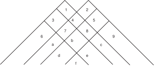
$n$$n$$n+1$$2n-1$$n+1$$1$$2n$$2n$$1$$n$$2n+1$$n$$n+1$$n+1$$1$

Figure 1. The image of $\mathcal{L}(\mathcal{K}_{(r,s)})\to\mathbb{Z}^{2}:L\mapsto(\operatorname{r}(L),\operatorname{tb}(L))$ for non-simple cablings of the positive trefoil with $\frac{s}{r}\in(n,n+1)$. The number of Legendrian knots realizing each point in $\mathbb{Z}^{2}$ whose coordinates sum to an odd number is indicated in the figure. The exact width of each region is determined by Theorem 1.7.

The transverse classification is now an immediate corollary.

Theorem 1.8.

Let $\mathcal{K}$ be the $(2,3)$-torus knot. If $\frac{s}{r}\not\in(1,\infty)$ then $\mathcal{K}_{(r,s)}$ is transversely simple and all transverse knots are stabilizations of the one with maximal self-linking number $rs+s-r$.

If $\frac{s}{r}\in[n,n+1)$ for a positive integer $n$ then $\mathcal{K}_{(r,s)}$ is not transversely simple and has the following classification.

1. The maximal self-linking number is $rs+s-r,$ and there is a unique transverse knot in $\mathcal{T}(\mathcal{K}_{(r,s)})$ with this self-linking number.

2. There are $n-1$ distinct transverse knots in $\mathcal{T}(\mathcal{K}_{(r,s)})$ that do not destabilize and have self-linking number $rs+r-s.$

3. If $\frac{r}{s}\not=n$ then there is a unique transverse knot in $\mathcal{T}(\mathcal{K}_{(r,s)})$ that does not destabilize and has self-linking number $rs+r-s-2|(n+1)r-s|$.

4. All other transverse knots in $\mathcal{T}(\mathcal{K}_{(r,s)})$ destabilize to one of the ones listed above.

5. None of the transverse knots listed above become transversely isotopic until they have been stabilized to have self-linking number $rs-s-r.$ There is a unique transverse knot in $\mathcal{T}(\mathcal{K}_{(r,s)})$ with self-linking number less than or equal to $rs-s-r.$

For the classification of cables of other positive torus knots we need some notation. Given a rational number $u=\frac{s}{r}>0$ let $u^{a}$ be the largest rational number with an edge in the Farey tessellation to $u.$ See Figure 2. (The $a$ superscript stands for ”anti-clockwise”, as $u^{a}$ is anti-clockwise of $u$ in the Farey tessellation.) Similarly the smallest rational number with an edge in the Farey tessellation to $u$ will be denoted by $u^{c}.$ A formula for computing these numbers will be given in Subsection 2.1. We will refer to the interval $(u^{c},u^{a})$ as the interval of influence for $u$.

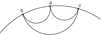
$u$$u^{a}$$u^{c}$

Figure 2. Given a rational number $u$, the numbers $u^{a}$ and $u^{c}$ are determined by the above figure in the Farey tessellation.

Given a positive $(p,q)$-torus knot and $k$ a positive integer, define

$$e_{k}=\frac{k}{pq-p-q}$$

We will see in Subsection 1.2 that such $e_{k}$ represent boundary slopes of non-thickenable solid tori, and that the half-intervals of influence $(e_{k},e_{k}^{a})$ will represent boundary slopes of partially thickenable solid tori when $\gcd{(k,pq-p-q)}=1$. We will refer to the $e_{k}$ as exceptional slopes. If we think of the fractions $e_{k}^{*}$ as representing curves on a torus, we denote the homological intersection of $(r,s)$ curves with the $e_{k}^{*}$ curves by

$$\frac{s}{r}\cdot e_{k}^{*}.$$

We can now state the precise classification theorems for cables of general positive $(p,q)$-torus knots.

Theorem 1.9.

Let $\mathcal{K}$ be a $(p,q)$-torus knot with $(p,q)\not=(2,3)$. Let

$$\mathcal{I}=\{n\in\mathbb{Z}:n>1\text{ and }\gcd(n,pq-p-q)=1\}$$

and

$$J=\cup_{n\in\mathcal{I}}J_{n}$$

where $J_{n}=(e_{n}^{c},e_{n}^{a})$ is the interval of influence for the exceptional slope $e_{n}$ defined above. The $J_{n}$ are all disjoint.

The classification of Legendrian knots in the knot type $\mathcal{K}_{(r,s)}$ is then given as follows.

1. If $\frac{s}{r}\not\in J$ then $\mathcal{K}_{(r,s)}$ is Legendrian simple. Moreover, in this case we have the following classification.

   1. If $\frac{s}{r}\in(0,\frac{1}{pq-p-q}]$ then there is a unique Legendrian knot $L\in\mathcal{L}(\mathcal{K}_{(r,s)})$ with Thurston-Bennequin invariant $\operatorname{tb}(L)=rs+s(pq-p-q)-r$ and rotation number $r(L)=0.$ All others are stabilizations of $L.$

   2. If $\frac{s}{r}>\frac{1}{pq-p-q}$ or $\frac{s}{r}<0$, then the maximal Thurston-Bennequin invariant for a Legendrian knot in $\mathcal{L}(\mathcal{K}_{(r,s)})$ is $rs$ and the rotation numbers realized by Legendrian knots with this Thurston-Bennequin invariant are

      $$\{\pm(r+s(n+k))\mbox{ }|\mbox{ }k=(pq-p-q-n),(pq-p-q-n)-2,\ldots,-(pq-p-q-n)\},$$

      where $n$ is the least integer bigger than $\frac{r}{s}$. All other Legendrian knots $L\in\mathcal{L}(\mathcal{K}_{(r,s)})$ are stabilizations of these. Two Legendrian knots with the same $\operatorname{tb}$ and $\operatorname{r}$ are Legendrian isotopic.

2. If $\frac{s}{r}\in J_{n}$ then there is some $k\geq 0$ such that $\frac{1}{k-1}>\frac{s}{r}>\frac{1}{k}$ and $\mathcal{K}_{(r,s)}$ is not Legendrian simple. The classification of Legendrian knots in $\mathcal{K}_{(r,s)}$ is as follows.

   1. The maximal Thurston-Bennequin invariant of $K_{(r,s)}$ is $rs$.

   2. For each integer $i$ in the set

      $$\{\pm(r+s(-k+l))\mbox{ }|\mbox{ }l=(pq-p-q-k),(pq-p-q-k)-2,\ldots,-(pq-p-q-k)\},$$

      there is a Legendrian $L_{i}\in\mathcal{L}(\mathcal{K}_{(r,s)})$ with

      $$\operatorname{tb}(L_{i})=rs\,\,\text{ and }\operatorname{r}(L_{i})=i.$$

   3. There are two Legendrian knots $K_{\pm}\in\mathcal{L}(\mathcal{K}_{(r,s)})$ satisfying

      $$\operatorname{tb}(K_{\pm})=rs\,\,\text{ and }\operatorname{r}(K_{\pm})=\pm(r-s(pq-p-q))$$

      if $\frac{s}{r}\in[e_{n},e_{n}^{a})$; however, if $\frac{s}{r}\in(e_{n}^{c},e_{n})$ then

      $$\operatorname{tb}(K_{\pm})=rs-\left|\frac{s}{r}\cdot e_{n}\right|\,\,\text{ and }\operatorname{r}(K_{\pm})=\pm r(n-1)$$

      and $K_{\pm}$ is not destabilizable.

   4. All Legendrian knots in $\mathcal{L}(\mathcal{K}_{(r,s)})$ destabilize to one of the $L_{i}$ or $K_{\pm}.$

   5. Let

      $$c=\begin{cases}(\frac{s}{r}\cdot e_{n}^{a})-1&\frac{s}{r}\in[e_{n},e_{n}^{a})\\ (\frac{s}{r}\cdot e_{n}^{a}-\frac{s}{r}\cdot e_{n})-1&\frac{s}{r}\in(e_{n}^{c},e_{n}).\end{cases}$$

      For any $y\in\mathbb{N}\cup\left\{0\right\}$ and $x\leq c$ the Legendrian $S_{\pm}^{x}S_{\mp}^{y}(K_{\pm})$ is not isotopic to a stabilization of any of the $L_{i}$ or $K_{\mp}$.

   6. Any two stabilizations of the non-destabilizable Thurston-Bennequin invariant Legendrian knots in $\mathcal{L}(\mathcal{K}_{(r,s)})$, except those mentioned in item (2e), are Legendrian isotopic if they have the same $\operatorname{tb}$ and $\operatorname{r}$.

From this theorem we can easily derive the transverse classification.

Theorem 1.10.

Let $\mathcal{K}$ be a $(p,q)$-torus knot with $(p,q)\not=(2,3)$. Using notation from Theorem 1.9 we have the following classification of transverse knots in $\mathcal{T}(\mathcal{K}_{(r,s)})$.

1. If $\frac{s}{r}\not\in J_{n}$ for any $n\in\mathcal{I}$ then $\mathcal{K}_{(r,s)}$ is transversely simple and all transverse knots in this knot type are stabilizations of the one with self-linking number $rs-r+s(pq-p-q)$.

2. If $\frac{s}{r}\in J_{n}$ for some $n\in\mathcal{I}$ then $\mathcal{K}_{(r,s)}$ is not transversely simple. There is a unique transverse knot $T$ in this knot type with maximal self-linking number, which is $rs-r+s(pq-p-q)$. There is also a unique non-destabilizable knot $T^{\prime}$ in this knot type and it has self-linking number $rs+r-s(pq-p-q)$. All other transverse knots in $\mathcal{T}(\mathcal{K}_{(r,s)})$ destabilize to either $T$ or $T^{\prime}$ and the stabilizations of $T$ and $T^{\prime}$ stay non-isotopic until they are stabilized to the point that their self-linking numbers are

   $$rs+r-s(pq-p-q)-2\left(\frac{s}{r}\cdot e_{n}^{a}\right)$$

   in the case of $\frac{s}{r}\in[e_{n},e_{n}^{a})$, and

   $$rs+r-s(pq-p-q)-2\left(\frac{s}{r}\cdot e_{n}^{a}-\frac{s}{r}\cdot e_{n}\right)$$

   in the case of $\frac{s}{r}\in(e_{n}^{c},e_{n})$.

We now turn from classification results for cables of positive torus knots, to classification results for embeddings of solid tori representing the positive torus knots themselves.

1.2. Classification results for solid tori

Let $S$ be a solid torus in a manifold $M.$ We say $S$ is in the knot type $\mathcal{K}$, or represents $\mathcal{K}$, if the core curve of $S$ is in the knot type $\mathcal{K}.$

We say a solid torus $S$ with convex boundary in a contact manifold $(M,\xi)$ thickens if there is a solid torus $S^{\prime}$ that contains $S$ such that $S^{\prime}$ has convex boundary with dividing slope different from $S.$ The existence of non-thickenable tori was first observed in [7]; the following theorem shows that non-thickenable tori exist for all positive $(p,q)$-torus knots.

Theorem 1.11.

Let $S$ be a solid torus in the knot type of a positive $(p,q)$-torus knot. In the standard tight contact structure $\xi_{std}$ on $S^{3}$ suppose that $\partial S$ is convex with two dividing curves of slope $\frac{s}{r}.$ Then $S$ thickens unless $\frac{s}{r}$ is an exceptional slope

$$e_{k}=\frac{k}{pq-p-q},$$

for some positive integer $k,$ in which case it might or might not thicken.

Moreover for each positive integer $k>1$ there are, up to contact isotopy, exactly two solid tori $N_{k}^{\pm}$ with convex boundary having $2n_{k}$ dividing curves of slope $e_{k}$ that do not thicken, where $n_{k}=\gcd(pq-p-q,k)$. For $k=1$ there is exactly one solid torus $N_{1}$ with convex boundary having two dividing curves of slope $e_{1}.$ This solid torus is a standard neighborhood of a Legendrian $(p,q)$-torus knots with maximal Thurston-Bennequin invariant and it does not thicken.

A key feature in the knot classification results above in Subsection 1.1 is a complete understanding of not only non-thickenable tori but also partially thickenable tori, that is tori with convex boundary that thicken, but not to a maximally thick torus in the given knot type. The existence of such tori has not been observed before, but it is clear that such tori will be key to future Legendrian classification results. In addition it is likely they will be important in understanding contact surgeries. The following theorem shows that partially thickenable tori exist for all positive $(p,q)$-torus knots.

Theorem 1.12.

Let $\mathcal{K}$ be a positive $(p,q)$-torus knot and let $e_{k}=\frac{k}{pq-p-q}$ be the exceptional slopes. Let $I_{k}=[e_{k},e_{k}^{a})$ and $\mathcal{I}=\{n\in\mathbb{Z}:n>1\text{ and }\gcd(n,pq-p-q)=1\}$. All solid tori below will represent the knot type $\mathcal{K}$.

1. If $(p,q)=(2,3)$ then $\mathcal{I}=\mathbb{N}-\left\{1\right\}$ and we have the following.

   1. The intervals $I_{k}=(k,\infty),$ so $I_{k}\subset I_{k+1}.$

   2. Any solid torus $S$ with convex boundary thickens to $N_{k}^{\pm}$ or to $N_{1}$ (that is a neighborhood of the maximal Thurston-Bennequin invariant $(2,3)$-torus knot).

   3. Any solid torus inside $N_{k}^{\pm}$ with convex boundary having dividing slope greater than $k$ (that is in $I_{k}$) does not thicken past the slope $e_{k}.$

   4. Any solid torus inside $N_{k}^{\pm}$ with convex boundary having negative (or infinite) dividing slope will thicken to a neighborhood of the maximal Thurston-Bennequin invariant $(2,3)$-torus knot.

2. If $(p,q)\not=(2,3)$ then we have the following.

   1. For any $k\not\in\mathcal{I}$, any solid torus $S$ inside $N_{k}^{\pm}$ with either boundary slope different from $e_{k}$, or less than $2n_{k}$ dividing curves, thickens to $N_{1}$.

   2. All the $I_{k}$ with $k\in\mathcal{I}$ are disjoint.

   3. Any solid torus $S$ with convex boundary having dividing slope in $I_{k}$ thickens to $N_{k}^{\pm}$ or to $N_{1}$ (that is a neighborhood of the maximal Thurston-Bennequin invariant $(p,q)$-torus knot).

   4. Any solid torus inside $N_{k}^{\pm}$ for some $k\in\mathcal{I}$, and with convex boundary having dividing slope in $I_{k}$, does not thicken past the slope $e_{k}.$

   5. Any solid torus inside $N_{k}^{\pm}$ with convex boundary having dividing slope outside of $I_{k}$ (that is greater than or equal to $e_{k}^{a}$ or negative) will thicken to a neighborhood of the maximal Thurston-Bennequin invariant $(p,q)$-torus knot.

From this theorem we can classify solid tori in the knot types of positive torus knots.

Corollary 1.13.

Let $\mathcal{K}$ be a positive $(p,q)$-torus knot and let $e_{k}=\frac{k}{pq-p-q}$ be the exceptional slopes. Let $I_{k}=[e_{k},e_{k}^{a})$ and $\mathcal{I}=\{n\in\mathbb{Z}:n>1\text{ and }\gcd(n,pq-p-q)=1\}$.

1. If $(p,q)=(2,3)$, then given a slope $s>1$ there is some integer $n$ such that $n\leq s<n+1$ and there are exactly $2n$ solid tori representing the knot type $\mathcal{K}$ with convex boundary having dividing slope $s$ and two dividing curves, only two of which thicken to a standard neighborhood of a Legendrian knot.

2. If $(p,q)\not=(2,3)$, then given any slope $s\geq\frac{1}{pq-p-q}$ we have the following.

   1. If there is some integer $n>0$ such that $\frac{1}{n}<s<\frac{1}{n-1}$ and $s\not\in I_{k}$ for any $k\in\mathcal{I}$, then there are exactly $2(pq-p-q-n+1)$ solid tori representing the knot type $\mathcal{K}$ with convex boundary having dividing slope $s$ and two dividing curves each of which thickens to a standard neighborhood of a Legendrian knot with $\operatorname{tb}=n$.

   2. If there is some integer $n>0$ such that $\frac{1}{n}<s<\frac{1}{n-1}$ and $s\in I_{k}$ for any $k\in\mathcal{I}$, then there are exactly $2(pq-p-q-n+1)+2$ solid tori representing the knot type $\mathcal{K}$ with convex boundary having dividing slope $s$ and two dividing curves, all but two of which thicken to a standard neighborhood of a Legendrian knot with $\operatorname{tb}=n$.

   3. If there is some $n>0$ such that $s=\frac{1}{n}$, then there are exactly $pq-p-q-n+1$ solid tori representing the knot type $\mathcal{K}$ with convex boundary having dividing slope $s$ and two dividing curves and they each represent a standard neighborhood of a Legendrian knot with $\operatorname{tb}=n$.

3. Given any negative slope $s$ there is some negative integer $n<0$ such that $\frac{1}{n+1}<s<\frac{1}{n}$. A solid torus with convex boundary having dividing slope $s$ and two dividing curves will thicken to a solid torus that is a standard neighborhood of a $\operatorname{tb}=n+1$ Legendrian knot.

We conclude this introduction with an outline of what follows. In Section 2 we collect needed preliminaries, including facts about continued fractions and convex surfaces, and we outline a strategy for classifying Legendrian knots. In Section 3 we classify embeddings of solid tori representing positive torus knots. In Section 4 we provide classifications for all simple cables of positive torus knots, and in Sections 5 and  6 we establish classifications for all non-simple cables of positive torus knots.

Acknowledgments. The first and third authors were partially supported by NSF Grant DMS-0804820. The second author was partially supported by QGM (Centre for Quantum Geometry of Moduli Spaces) funded by the Danish National Research Foundation. Some of the work presented in this paper was carried out in the Spring of 2010 while the first and third author were at MSRI, we gratefully acknowledge their support for this work.

2. Preliminaries

In this section we first prove some important facts about continued fractions in Subsection 2.1. The remaining sections recall various facts concerning the classification of Legendrian and transverse knots from [5]. The reader is assumed to be familiar with the basic notions associated to convex surfaces and Legendrian and transverse knots, but these sections are included for the convenience of the reader and to make the paper as self-contained as possible. All this information can be found in [5, 9].

2.1. Continued fractions, the Farey tessellation, and intersection of curves on a torus

In this section we collect various facts about continued fractions and the Farey tessellation (see Figure 4) that will be needed throughout our work.

Given a rational number $u>0$ we may represent it as a continued fraction

$$u=a_{0}-\cfrac{1}{a_{1}-\cfrac{1}{a_{2}\ldots-\cfrac{1}{a_{n}}}}$$

with $a_{0}\geq 1$ and the other $a_{i}>1$. We will denote this as $u=[a_{0};a_{1},\ldots,a_{n}]$. If we know that $u=[a_{0};a_{1},\ldots,a_{n}]$ then we define

$$u^{a}=[a_{0};a_{1},\ldots,a_{n-1}],$$

with the convention that if $n=0$ then $u^{a}=\infty$; we also define

$$u^{c}=[a_{0};a_{1},\ldots,a_{n}-1].$$

Lemma 2.1.

The number $u^{a}$ is the largest rational number bigger than $u$ with an edge to $u$ in the Farey tessellation and $u^{c}$ is the smallest rational number less than $u$ with an edge to $u$ in the Farey tessellation. Moreover there is an edge in the Farey tessellation between $u^{a}$ and $u^{c}$ and $u$ is the mediant of $u^{a}$ and $u^{c}$, that is if $u^{a}=\frac{p^{a}}{q^{a}}$ and $u^{c}=\frac{p^{c}}{q^{c}}$ then

$$u=\frac{p^{a}+p^{c}}{q^{a}+q^{c}}.$$

Proof.

Define $\frac{p_{k}}{q_{k}}=[a_{0};a_{1},\ldots,a_{k}]$ and $p_{-1}=1,q_{-1}=0.$ One may easily verify using induction that

$$p_{k+1}=a_{k+1}p_{k}-p_{k-1},\text{ and }\,q_{k+1}=a_{k+1}q_{k}-q_{k-1}.$$

From this one can inductively deduce that

$$p_{k+1}q_{k}-p_{k}q_{k+1}=-1.$$

Thus there is an edge in the Farey tessellation between $u=\frac{p}{q}=\frac{p_{n}}{q_{n}}$ and $u^{a}=\frac{p^{a}}{q^{a}}=\frac{p_{n-1}}{q_{n-1}}.$ Similarly, let $\frac{c_{k}}{d_{k}}=[a_{k};a_{k+1},\ldots,a_{n}]$ and $\frac{c^{\prime}_{k}}{d^{\prime}_{k}}=[a_{k};a_{k+1},\ldots,a_{n}-1]$ and notice that $c_{n}d^{\prime}_{n}-d_{n}c^{\prime}_{n}=a_{n}-(a_{n}-1)=1.$ Now we see that

$$\frac{c_{k}}{d_{k}}=a_{k}-\frac{1}{c_{k+1}/{d_{k+1}}}=\frac{a_{k}c_{k+1}-d_{k+1}}{c_{k+1}}$$

and a similar expression for $\frac{c^{\prime}_{k}}{d^{\prime}_{k}}$ and induction yield $c_{k}d^{\prime}_{k}-d_{k}c^{\prime}_{k}=1.$ In particular, there is an edge in the Farey tessellation between $u=\frac{c_{0}}{d_{0}}$ and $u^{c}=\frac{c^{\prime}_{0}}{d^{\prime}_{0}}.$

Finally by setting $\frac{c^{\prime\prime}_{k}}{d^{\prime\prime}_{k}}=[a_{k};a_{k+1},\ldots,a_{n-1}]$ and noticing that $c^{\prime\prime}_{n-1}d^{\prime}_{n-1}-d^{\prime\prime}_{n-1}c^{\prime}_{n-1}=1$, we can use the above formulas, and analogous ones, to inductively prove that $c^{\prime\prime}_{k-1}d^{\prime}_{k-1}-d^{\prime\prime}_{k-1}c^{\prime}_{k-1}=1$. This establishes an edge in the Farey tessellation between $u^{c}=\frac{c^{\prime}_{0}}{d^{\prime}_{0}}$ and $u^{a}=\frac{c^{\prime\prime}_{0}}{d^{\prime\prime}_{0}}$. Since there is an edge in the Farey tessellation between each pair of numbers in the set $\{u,u^{a},u^{c}\}$ the lemma is established by noticing that the numerators (and denominators) of $u^{a}$ and $u^{c}$ are both smaller than the numerator (and denominator) of $u.$ ∎

We recall that if we choose a basis for $H_{1}(T^{2};\mathbb{Z})$ then there is a one-to-one correspondence between embedded essential oriented curves on $T^{2}$ and rational numbers $\frac{p}{q}$, written in lowest common terms. Moreover given two rational numbers $\frac{p}{q}$ and $\frac{r}{s}$ we denote their homological intersection (which also happens to be the signed minimal intersection number) between the corresponding curves on $T^{2}$ by $\frac{p}{q}\cdot\frac{r}{s}$ and it can be computed by

$$\frac{p}{q}\cdot\frac{r}{s}=ps-rq.$$

Notice that this number is only well defined up to sign (since the orientation on the curve corresponding to a fraction is not determined). Throughout this work we will only be concerned with the absolute value of this number (if the exact number is ever needed we will specify the orientations on the homology class corresponding to a fraction).

Lemma 2.2.

Fix some positive integer $n$ and set $e_{k}=\frac{k}{n}$ for $k\in\left\{1,2,\ldots\right\}$ and $\mathcal{I}=\{k\in\mathbb{Z}:k>1\text{ and }\gcd(n,k)=1\}$. If $n\not=1$ then the intervals $J_{k}=(e_{k}^{c},e_{k}^{a})$ for $k\in\mathcal{I}$ are all disjoint. If $n=1$ then the intervals are nested $J_{k+1}\subset J_{k}$.

If $r$ is a positive rational number less than $e_{k}^{c}$ or greater than $e_{k}^{a}$ then for any $s\in\overline{J_{k}}$ we have

$$|r\cdot s|\geq\min\{|r\cdot e_{k}^{a}|,|r\cdot e_{k}^{c}|\}$$

with equality only if $s=e_{k}^{a}$ or $e_{k}^{c}$.

If $r\in(e_{k}^{c},e_{k})$ and $s\in(e_{k},e_{k}^{a}),$ then

$$|r\cdot s|>|r\cdot e_{k}^{a}|.$$

Proof.

If $n=1$ then it is clear that $e_{k}=k$ and one easily checks that $e_{k}^{c}=k-1$ and $e_{k}^{a}=\infty.$ So $J_{k}=(k-1,\infty)$.

If $n\not=1$ then we notice that any number in $(e^{c}_{k},e_{k})$ is a mediant of $e_{k}$ and $e_{k}^{c}$ and hence has denominator strictly bigger than $n$ (since the denominator of $e_{k}$ is $n$), thus $e_{k^{\prime}}$ cannot be in this interval for any $k^{\prime}\in\mathcal{I}$. Similarly $e_{k^{\prime}}$ cannot be in the interval $(e_{k},e_{k}^{a})$. Thus the intervals $J_{k},i\in\mathcal{I}$ are disjoint.

For the second statement notice that $r\cdot e_{k}^{a}$ and $r\cdot e_{k}^{c}$ have the same sign and $r\cdot s$ will be some non-negative integral linear combination of $r\cdot e_{k}^{a}$ and $r\cdot e_{k}^{c}$. For the last statement note that $r\cdot s$ will be some positive integral linear combination of $r\cdot e_{k}$ and $r\cdot e_{k}^{a}$. ∎

2.2. Convex surfaces and bypasses

In this subsection we discuss the main tools we will be using throughout the paper — convex surfaces. We assume the reader is familiar with convex surfaces as used in [5, 9]; but, for the convenience of the reader, we recall the fundamental facts from the theory that we will use in this paper.

2.2.1. Convex surfaces

Recall a surface $\Sigma$ in a contact manifold $(M,\xi)$ is convex if it has a neighborhood $\Sigma\times I$, where $I=(-\epsilon,\epsilon)$ is some interval, and $\xi$ is $I$-invariant in this neighborhood. Any closed surface can be $C^{\infty}$-perturbed to be convex. Moreover if $L$ is a Legendrian knot on $\Sigma$ for which the contact framing is non-positive with respect to the framing given by $\Sigma$, then $\Sigma$ may be perturbed in a $C^{0}$ fashion near $L$, but fixing $L$, and then again in a $C^{\infty}$ fashion away from $L$ so that $\Sigma$ is convex.

Given a convex surface $\Sigma$ with $I$-invariant neighborhood let $\Gamma_{\Sigma}\subset\Sigma$ be the multicurve where $\xi$ is tangent to the $I$ factor. This is called the dividing set of $\Sigma.$ If $\Sigma$ is oriented it is easy to see that $\Sigma\setminus\Gamma=\Sigma_{+}\cup\Sigma_{-}$ where $\xi$ is positively transverse to the $I$ factor along $\Sigma_{+}$ and negatively transverse along $\Sigma_{-}$. If $L$ is a Legendrian curve on a $\Sigma$ then the framing of $L$ given by the contact planes, relative to the framing coming from $\Sigma$, is given by $-\frac{1}{2}(L\cdot\Gamma)$. Moreover if $L=\partial\Sigma$ then the rotation number of $L$ is given by $\operatorname{r}(L)=\chi(\Sigma_{+})-\chi(\Sigma_{-})$.

2.2.2. Convex tori

A convex torus $T$ is said to be in standard form if $T$ can be identified with $\mathbb{R}^{2}/\mathbb{Z}^{2}$ so that $\Gamma_{T}$ consists of $2n$ vertical curves (note $\Gamma_{T}$ will always have an even number of curves and we can choose a parameterization to make them vertical) and the characteristic foliations consists of $2n$ vertical lines of singularities ($n$ lines of sources and $n$ lines of sinks) and the rest of the foliation is by non-singular lines of slope $s$. See Figure 3.

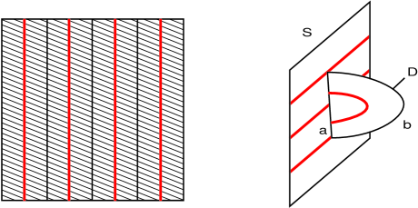
$D$$\Sigma$$\alpha$$\beta$

Figure 3. Standard convex tori shown on the left and a bypass shown on the right. The thicker curves are dividing curves.

The lines of singularities are called Legendrian divides and the other curves are called ruling curves. We notice that the Giroux Flexibility Theorem allows us to isotope any convex torus into standard form, [5, 9].

2.2.3. Bypasses and tori

Let $\Sigma$ be a convex surface and $\alpha$ a Legendrian arc in $\Sigma$ that intersects the dividing curves $\Gamma_{\Sigma}$ in 3 points $p_{1},p_{2},p_{3}$ (where $p_{1},p_{3}$ are the end points of the arc). Then a bypass for $\Sigma$ (along $\alpha$), see Figure 3, is a convex disk $D$ with Legendrian boundary such that

1. $D\cap\Sigma=\alpha,$

2. $tb(\partial D)=-1,$

3. $\partial D=\alpha\cup\beta,$

4. $\alpha\cap\beta=\{p_{1},p_{3}\}$ are corners of $D$ and elliptic singularities of $D_{\xi}.$

A surface $\Sigma$ locally separates the ambient manifold. If a bypass is contained in the (local) piece of $M\setminus\Sigma$ that has $\Sigma$ as its oriented boundary then we say the bypass will be attached to the front of $\Sigma$ otherwise we say it is attached to the back of $\Sigma$.

When a bypass is attached to a torus $T$ then either the dividing curves do not change, their number increases by two, or decreases by two, or the slope of the dividing curves changes. The slope of the dividing curves can change only when there are two dividing curves. (See [9] for more details.) If the bypass is attached to $T$ along a ruling curve then either the number of dividing curves decreases by two or the slope of the dividing curves changes. To understand the change in slope we need the following. Let $\mathbb{D}$ be the unit disk in $\mathbb{R}^{2}.$ Recall the Farey tessellation of $\mathbb{D}$ is constructed as follows. Label the point $(1,0)$ on $\partial\mathbb{D}$ by $0=\frac{0}{1}$ and the point $(-1,0)$ with $\infty=\frac{1}{0}.$ Now join them by a geodesic. If two points $\frac{p}{q},$ $\frac{p^{\prime}}{q^{\prime}}$ on $\partial\mathbb{D}$ with non-negative $y$-coordinate have been labeled then label the point on $\partial\mathbb{D}$ half way between them (with non-negative $y$-coordinate) by $\frac{p+p^{\prime}}{q+q^{\prime}}.$ Then connect this point to $\frac{p}{q}$ by a geodesic and to $\frac{p^{\prime}}{q^{\prime}}$ by a geodesic. Continue this until all positive fractions have been assigned to points on $\partial\mathbb{D}$ with non-negative $y$-coordinates. Now repeat this process for the points on $\partial\mathbb{D}$ with non-positive $y$-coordinate except start with $\infty=\frac{-1}{0}.$ See Figure 4.

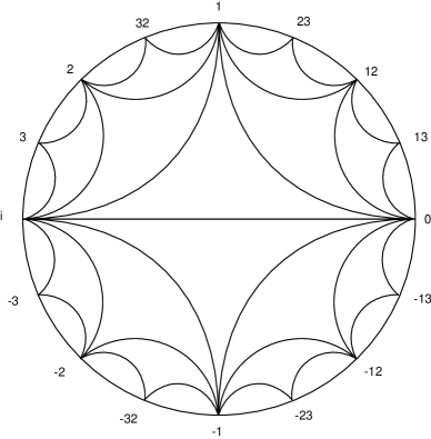
0$\infty$$1$23$-1$$-2$$-3$$\frac{1}{2}$$\frac{1}{3}$$-\frac{1}{2}$$-\frac{1}{3}$$\frac{2}{3}$$-\frac{2}{3}$$\frac{3}{2}$$-\frac{3}{2}$

Figure 4. The Farey tessellation.

The key result we need to know about the Farey tessellation is given in the following theorem.

Theorem 2.3 (Honda 2000, [9]).

Let $T$ be a convex torus in standard form with $|\Gamma_{T}|=2,$ dividing slope $s$ and ruling slope $r\not=s.$ Let $D$ be a bypass for $T$ attached to the front of $T$ along a ruling curve. Let $T^{\prime}$ be the torus obtained from $T$ by attaching the bypass $D.$ Then $|\Gamma_{T^{\prime}}|=2$ and the dividing slope $s^{\prime}$ of $\Gamma_{T^{\prime}}$ is determined as follows: let $[r,s]$ be the arc on $\partial\mathbb{D}$ running from $r$ counterclockwise to $s,$ then $s^{\prime}$ is the point in $[r,s]$ closest to $r$ with an edge to $s.$

If the bypass is attached to the back of $T$ then the same algorithm works except one uses the interval $[s,r]$ on $\partial\mathbb{D}$. ∎

2.2.4. The Imbalance Principle

As we see that bypasses are useful in changing dividing curves on a surface we mention a standard way to try to find them called the Imbalance Principle. Suppose that $\Sigma$ and $\Sigma^{\prime}$ are two disjoint convex surfaces and $A$ is a convex annulus whose interior is disjoint from $\Sigma$ and $\Sigma^{\prime}$ but its boundary is Legendrian with one component on each surface. If $|\Gamma_{\Sigma}\cdot\partial A|>|\Gamma_{\Sigma^{\prime}}\cdot A|$ then there will be a dividing curve on $A$ that cuts a disk off of $A$ that has part of its boundary on $\Sigma$. It is now easy to use the Giroux Flexibility Theorem to show that there is a bypass for $\Gamma$ on $A$.

2.2.5. Discretization of Isotopy

We will frequently need to analyze what happens to the contact geometry when we have a topological isotopy between two convex surfaces $\Sigma$ and $\Sigma^{\prime}$. This can be done by the technique of Isotopy Discretization [2] (see also [5] for its use in studying Legendrian knots). Given an isotopy between $\Sigma$ and $\Sigma^{\prime}$ one can find a sequence of convex surfaces $\Sigma_{1}=\Sigma,\Sigma_{2},\ldots,\Sigma_{n}=\Sigma^{\prime}$ such that

1. all the $\Sigma_{i}$ are convex and

2. $\Sigma_{i}$ and $\Sigma_{i+1}$ are disjoint and $\Sigma_{i+1}$ is obtained from $\Sigma_{i}$ by a bypass attachment.

Thus if one is trying to understand how the contact geometry of $M\setminus\Sigma$ and $M\setminus\Sigma^{\prime}$ relate, one just needs to analyze how the contact geometry of the pieces of $M\setminus\Sigma_{i}$ changes under bypass attachment. In particular, many arguments can be reduced from understanding a general isotopy to understanding an isotopy between two surfaces that cobound a product region.

There is also a relative version of Isotopy Discretization where $\Sigma$ and $\Sigma^{\prime}$ are convex surfaces with Legendrian boundary consisting of ruling curves on a convex torus. If $\partial\Sigma=\partial\Sigma^{\prime}$ and there is a topological isotopy of $\Sigma$ to $\Sigma^{\prime}$ relative to the boundary then we can find a discrete isotopy as described above.

2.3. Classifying knots in a knot type

In this section we briefly recall the standard strategy for classifying Legendrian knots in a given knot type $\mathcal{K}$ as laid out in [4, 5]. We begin by recalling the “normal form” for a neighborhood of a Legendrian or transverse knot and the relation between them.

2.3.1. Standard neighborhoods of knots

Given a Legendrian knot $L$, a standard neighborhood of $L$ is a solid torus $N$ that has convex boundary with two dividing curves of slope $1/\operatorname{tb}(L)$ (and of course we will usually take $\partial N$ to be a convex torus in standard form). Conversely given any such solid torus it is a standard neighborhood of a unique Legendrian knot. Up to contactomorphism one can model a standard neighborhood as a neighborhood $N^{\prime}$ of the $x$-axis in $\mathbb{R}^{3}/(x\mapsto x+1)\cong S^{1}\times\mathbb{R}^{2}$ with contact structure $\xi_{std}=\ker(dz-y\,dx).$ Using this model we can see that $L_{\pm}=\{(x,\pm\epsilon,0)\}\subset N^{\prime}$ is a $(\pm)$-transverse curve. The image of $L_{+}$ in $N$ is called the transverse push-off of $L$ and $L_{-}$ is called the negative transverse push-off. One may easily check that $L_{\pm}$ is well-defined and compute that

$${\,sl}(L_{\pm})=\operatorname{tb}(L)\mp\operatorname{r}(L).$$

One may understand stabilizations and destabilizations of a Legendrian knot $K$ in terms of the standard neighborhood. Specifically, inside the standard neighborhood $N$ of $L$, $L$ can be positively stabilized to $S_{+}(L)$, or negatively stabilized to $S_{-}(L)$. Let $N_{\pm}$ be a neighborhood of the stabilization of $L$ inside $N.$ As above we can assume that $N_{\pm}$ has convex boundary in standard form. It will have dividing slope $\frac{1}{\operatorname{tb}(L)-1}.$ Thus the region $N\setminus N_{\pm}$ is diffeomorphic to $T^{2}\times[0,1]$ and the contact structure on it is easily seen to be a basic slice, see [9]. There are exactly two basic slices with given dividing curves on their boundary and as there are two types of stabilization of $L$ we see that the basic slice $N\setminus N_{\pm}$ is determined by the type of stabilization done, and vice versa. Moreover if $N$ is a standard neighborhood of $L$ then $L$ destabilizes if the solid torus $N$ can be thickened to a solid torus $N_{d}$ with convex boundary in standard form with dividing slope $\frac{1}{\operatorname{tb}(L)+1}.$ Moreover the sign of the destabilization will be determined by the basic slice $N_{d}\setminus N$. Finally, we notice that using Theorem 2.3 we can destabilize $L$ by finding a bypass for $N$ attached along a ruling curve whose slope is clockwise of $1/(\operatorname{tb}(L)+1)$ (and anti-clockwise of $0$).

A neighborhood of a transverse knot $T$ can be modeled by the solid torus $S_{a}=\{(\phi,(r,\theta))|r\leq a\}\subset S^{1}\times\mathbb{R}^{2}$ for sufficiently small $a$, where $(r,\theta)$ are polar coordinates on $\mathbb{R}^{2}$ and $\phi$ is the angular coordinate on $S^{1}$, with the contact structure $\xi_{cyl}=\ker(d\phi+r^{2}\,d\theta)$. Notice that the tori $\partial S_{b}$ inside of $S_{a}$ have linear characteristic foliations of slope $-b^{2}.$ Thus for all integers $n$ with $\frac{1}{\sqrt{n}}<a$ we have tori $T_{n}=\partial S_{1/\sqrt{n}}$ with linear characteristic foliation of slope $-\frac{1}{n}.$ Let $L_{n}$ be a leaf of the characteristic foliation of $T_{n}.$ Any Legendrian $L$ Legendrian isotopic to one of the $L_{n}$ so constructed will be called a Legendrian approximation of $T.$

Lemma 2.4 (Etnyre-Honda 2001, [5]).

If $L_{n}$ is a Legendrian approximation of the transverse knot $T$ then $(L_{n})_{+}$ is transversely isotopic to $T.$ Moreover, $L_{n+1}$ is Legendrian isotopic to the negative stabilization of $L_{n}.$∎

This lemma is a key ingredient in the following result from which our transverse classification results will follow from our Legendrian classification results.

Theorem 2.5 (Etnyre-Honda 2001, [5]).

The classification of transverse knots up to transverse isotopy is equivalent to the classification of Legendrian knots up to negative stabilization and Legendrian isotopy.

2.3.2. Classification strategy

The classification of Legendrian knots in a given knot type can be done in a (roughly) three step process.

Step I — Identify the maximal Thurston-Bennequin invariant of $\mathcal{K}$ and classify Legendrian knots realizing this.

Step II — Identify and classify the non-maximal Thurston-Bennequin Legendrian knots in $\mathcal{K}$ that do not destabilize and prove that all other knots destabilize to one of these identified knots.

Step III — Determine which stabilizations of the maximal Thurston-Bennequin invariant knots and non-destabilizable knots are Legendrian isotopic.

As stabilization of a Legendrian knot is well defined and positive and negative stabilizations commute, it is clear that these steps will yield a classification of Legendrian knots in the knot type $\mathcal{K}$.

Step II is facilitated by the observation above that bypasses attached to appropriate ruling curves of a standard neighborhood of a Legendrian knot yield destabilizations. Similarly, if $L$ is a Legendrian knot contained in a convex surface $\Sigma$ (and the framing given to $L$ by $\Sigma$ is less than or equal to the framing given by a Seifert surface) and there is a bypass for $L$ on $\Sigma$ then this leads to a destabilization of $L$. Moreover one can find such a bypass in some cases by the Imbalance Principle discussed above.

2.3.3. Contact isotopy and contactomorphism

We begin by recalling a result of Eliashberg concerning the contactomorphism group of the standard contact structure $\xi_{std}$ on $S^{3}$. Fix a point $p$ in $S^{3}$ and let $\hbox{\em Diff}_{0}(S^{3})$ be the group of orientation-preserving diffeomorphisms of $S^{3}$ that fix the plane $\xi_{std}(p),$ and let $\hbox{\em Diff}_{\xi_{std}}$ be the group of diffeomorphisms of $S^{3}$ that preserve $\xi_{std}$.

Theorem 2.6 (Eliashberg 1992, [3]).

The natural inclusion of

$$\hbox{Diff}_{\xi_{std}}\hookrightarrow\hbox{Diff}_{0}(S^{3})$$

is a weak homotopy equivalence. ∎

Using this fact it is clear that if one has a contactomorphism $\phi$ of $(S^{3},\xi_{std})$ that takes a set $S\subset S^{3}$ to $S^{\prime}\subset S^{3}$, then there is a contact isotopy of $(S^{3},\xi_{std})$ that takes $S$ to $S^{\prime}$. In particular, if one is trying to show that two embeddings of a contact structure on a torus are contact isotopic then one merely needs to construct a contactomorphism that takes one torus to the other. Similarly to show two Legendrian knots are Legendrian isotopic one only needs to construct a contactomorphism that takes one knot to the other (or takes a standard neighborhood of one of the knots to the other, that is understand the contactomorphism type of the complement of the standard neighborhood).

2.4. Computations of $\operatorname{tb},\operatorname{r}$ and $\overline{\operatorname{tb}}$

In this subsection we collect various facts that are useful in computing the classical invariants of Legendrian knots on tori.

2.4.1. Rotation numbers for curves on convex tori

Let $T$ be a convex torus in a contact manifold $(M,\xi),$ where $\xi$ has Euler class 0. Now we define an invariant of homology classes of curves on $T.$ Let $v$ be any globally non-zero section of $\xi$ and $w$ a section of $\xi|_{T}$ that is transverse to and twists (with $\xi$) along the Legendrian ruling curves and is tangent to the Legendrian divides. If $\gamma$ is a closed oriented curve on $T$ then set $f_{T}(\gamma)$ equal to the rotation of $v$ relative $w$ along $\gamma.$ One may check the following properties (cf. [4, 5]).

1. The function $f_{T}$ is well-defined on homology classes.

2. The function $f_{T}$ is linear.

3. The function $f_{T}$ is unchanged if we isotope $T$ through convex tori in standard form.

4. If $\gamma$ is a $(r,s)$-ruling curve or Legendrian divide then $f_{T}(\gamma)=r(\gamma).$

2.4.2. Legendrian knots on tori

We recall two simple lemmas from [7]. The first concerns the computation of the Thurston-Bennequin invariant for cables.

Lemma 2.7.

Let $\mathcal{K}$ be a knot type and $N$ a solid torus representing $\mathcal{K}$ whose boundary is a standard convex torus. Suppose that $L\in\mathcal{L}(\mathcal{K}_{(p,q)})$ is contained in $\partial N$.

1. Suppose $L_{(p,q)}$ is a Legendrian divide and $\mbox{slope}(\Gamma_{\partial N(\mathcal{K})})={\frac{q}{p}}$. Then

   $$\operatorname{tb}(L_{(p,q)})=pq.$$

2. Suppose $L_{(p,q)}$ is a Legendrian ruling curve and $\mbox{slope}(\Gamma_{\partial N(\mathcal{K})})={\frac{q^{\prime}}{p^{\prime}}}$. Then

   $$\operatorname{tb}(L_{(p,q)})=pq-|pq^{\prime}-qp^{\prime}|.$$

∎

A simple consequence of the discussion in Subsection 2.4.1 yields the following computation of the rotation number for cables.

Lemma 2.8.

Let $\mathcal{K}$ be a knot type and $N$ a solid torus representing $\mathcal{K}$ whose boundary is a standard convex torus. Suppose that $L\in\mathcal{L}(\mathcal{K}_{(p,q)})$ is contained in $\partial N$. Then

$$r(L_{(p,q)})=p\cdot r(\partial D)+q\cdot r(\partial\Sigma),$$

where $D$ is a convex meridional disk of $N$ with Legendrian boundary on a contact-isotopic copy of the convex surface $\partial N$, and $\Sigma$ is a convex Seifert surface with Legendrian boundary in $\mathcal{L}(\mathcal{K})$ which is contained in a contact-isotopic copy of $\partial N(\mathcal{K})$. ∎

We end with a lemma that was established as Claim 4.2 in [7]. Recall that the contact width of a knot type $\mathcal{K}$ is given by

$$w(\mathcal{K})=\textrm{sup}\frac{1}{\textrm{slope}(\Gamma_{\partial S})}$$

where here $S$ ranges over all solid tori with convex boundary representing $\mathcal{K}$.

Lemma 2.9.

Given a knot type $\mathcal{K}$, suppose $(r,s)$ is a pair of relatively prime integers such that $\frac{r}{s}<w(\mathcal{K})$. Then the maximal Thurston-Bennequin invariant of $\mathcal{K}_{(r,s)}$ is

$$\overline{\operatorname{tb}}(\mathcal{K}_{(r,s)})=rs.$$

∎

3. Solid tori in $S^{3}$

In Subsection 3.1 we classify non-thickenable tori in the knot types of the positive torus knots, and in Subsection 3.2 we classify the partially thickenable tori. Subsection 3.3 discusses Legendrian knots sitting on these tori as ruling curves and Legendrian dividing curves.

3.1. Non-thickenable tori

When considering tori $N$ that realize the knot type of $(p,q)$-torus knot $\mathcal{K},$ there are two different “natural” coordinates to use. The first is the longitude-meridian coordinates where the longitude comes from the intersection of a Seifert surface with $\partial N.$ This longitude will be called the $\infty$-longitude, and these coordinates will be called the $\mathcal{C}$ coordinates. The other coordinate system has the longitude given by the framing coming from the Heegaard torus that $\mathcal{K}$ sits on in $S^{3}.$ This longitude will be called the $\infty^{\prime}$-longitude and these coordinates will be called the $\mathcal{C}^{\prime}$ coordinates. Except where stated otherwise we will always use the more standard $\mathcal{C}$ coordinates.

Lemma 3.1.

Suppose that the solid torus $N$ represents the knot type of a positive $(p,q)$-torus knot $\mathcal{K}$. If $N$ has convex boundary then $N$ will thicken unless it has dividing slope

$$e_{k}=\frac{k}{pq-p-q}$$

for some $k\in\left\{1,2,\ldots\right\}$, and $2n_{k}$ dividing curves where $n_{k}=\gcd(pq-p-q,k).$

Proof.

We begin by ignoring the contact structure and building a topological model for the complement of $N.$ See Figure 5. The knot $\mathcal{K}$ can be thought to sit on a torus $T$ that separates $S^{3}$ into two solid tori $V_{1}$ and $V_{2}$, each of which can be thought of as a neighborhood of an unknot $F_{1}$ and $F_{2}.$ As $N$ is a neighborhood of $\mathcal{K}$, we can isotope $T$ so that it intersects $N$ in an annulus and thus $A^{\prime}=T\setminus(T\cap N)$ is an annulus in the complement of $N$ with boundary on $\partial N.$ Moreover, there is a small neighborhood of $A^{\prime},$ which we denote ${N}(A^{\prime})$ such that $S^{3}\setminus(N\cup{N}(A^{\prime}))$ consists of two solid tori, which we may think of as $V_{1}$ and $V_{2}.$ Turning this construction around $V_{1}\cup V_{2}\cup{N}(A^{\prime})$ is the complement of $N.$ We can identify $N(A^{\prime})$ as a neighborhood of an annulus $A$ that has one boundary component a $(p,q)$ curve on $\partial V_{1}$ and the other boundary component a $(q,p)$ curve on $\partial V_{2}.$ Thus, topologically, the complement of $N$ can be built as the neighborhood of two unknots (that form a Hopf link) union the neighborhood of an annulus $A.$

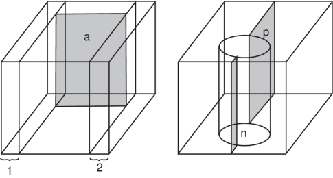
$V_{1}$$V_{2}$$A$$A^{\prime}$$N$

Figure 5. The cubes in the picture represent $T^{2}\times[0,1]$ (the top and bottom are identified and the front and back are also identified), thought of as the complement of the Hopf link $F_{1}\cup F_{2}$. We have chosen coordinates on the torus so that the $(p,q)$ curve is vertical. On the left hand side we see the solid tori $V_{1}$ and $V_{2}$ (minus their cores) and the annulus $A$. On the right hand side we see the solid torus $N$ and the annulus $A^{\prime}$.

Bringing the contact structure back into the picture we can assume that $L_{i}$, $i=1,2$, is a Legendrian representative of $F_{i}$ in the complement of $N,$ which maximize $tb(L_{i})$ in the complement of $N$, subject to the condition that $L_{1}\sqcup L_{2}$ is isotopic to $F_{1}\sqcup F_{2}$ in the complement of $N$. Let $tb(L_{i})=-m_{i}$, where $m_{i}>0.$ If $N(L_{i})$ is a regular neighborhood of $L_{i}$, then $\textrm{slope}(\Gamma_{\partial N(L_{i})})=-1/m_{i}$ with respect to $\mathcal{C}_{F_{i}}$.

Notice that $S^{3}\setminus(N(L_{1})\cup N(L_{2}))$ is diffeomorphic to $S=T^{2}\times[0,1]$ and contains $N.$ We wish to change coordinates on $T^{2}$ so that $N$ is a vertical solid torus in $S.$ Specifically, $T^{2}$ inherits coordinates as the boundary of $N(L_{1}),$ that is using the coordinate system coming from the framing $\mathcal{C}_{F_{1}}.$ We change coordinates so that the $(p,q)$ curve on $T^{2}$ becomes the $(0,1)$ curve (which can be thought of as the longitude in the $\mathcal{C}^{\prime}$ framing). This can be done by sending the oriented basis $((p,q),(p^{\prime},q^{\prime}))$ for $T^{2},$ where $pq^{\prime}-qp^{\prime}=1$, to the basis $((0,1),(-1,0)).$ This corresponds to the map $\displaystyle\phi_{1}=\left(\begin{array}[]{cc}q&-p\\ q^{\prime}&-p^{\prime}\end{array}\right)$. Then $\phi_{1}$ maps $(-m_{1},1)\mapsto(-qm_{1}-p,-q^{\prime}m_{1}-p^{\prime})$. Since we are only interested in slopes, we write this as $(qm_{1}+p,q^{\prime}m_{1}+p^{\prime})$.

Similarly, we change from $\mathcal{C}_{F_{2}}$ to $\mathcal{C}^{\prime}$. The only thing we need to know here is that $(-m_{2},1)$ maps to $(pm_{2}+q,p^{\prime}m_{2}+q^{\prime})$. Thus $S$ is a thickened torus $T^{2}\times[0,1]$ with dividing slope $\frac{q^{\prime}m_{1}+p^{\prime}}{qm_{1}+p}$ on $T\times\{0\}$ and $\frac{p^{\prime}m_{2}+q^{\prime}}{pm_{2}+q}$ on $T\times\{1\}.$

Now suppose $qm_{1}+p\neq pm_{2}+q$. This would mean that the twisting of Legendrian ruling representatives of $K$ on $\partial N(L_{1})$ and $\partial N(L_{2})$ would be unequal. Then we could apply the Imbalance Principle to a convex annulus ${A}$ in $S^{3}\backslash N$ between $\partial N(L_{1})$ and $\partial N(L_{2})$ to find a bypass along one of the $\partial N(L_{i})$. This bypass in turn gives rise to a thickening of $N(L_{i})$, allowing, by the twist number lemma [9], the increase of $tb(L_{i})$ by one. Hence, eventually we arrive at $qm_{1}+p=pm_{2}+q$ and a standard convex annulus ${A}$; that is, the dividing curves on $A$ run from one boundary component of $A$ to the other.

Since $m_{i}>0$, the smallest solution to $qm_{1}+p=pm_{2}+q$ is $m_{1}=m_{2}=1$. All the other positive integer solutions are therefore obtained by taking $m_{1}=pj+1$ and $m_{2}=qj+1$ with $j$ a non-negative integer. We can then compute the boundary slope of the dividing curves on $\partial(\widetilde{N})$ where $\widetilde{N}=N(L_{1})\cup N(L_{2})\cup{N}(A).$ This will be the boundary slope for the solid torus $\widetilde{N}$ containing $N$. We have

(3.1) $$-\frac{q^{\prime}(pj+1)+p^{\prime}}{pqj+p+q}+\frac{p^{\prime}(qj+1)+q^{\prime}}{pqj+p+q}-\frac{1}{pqj+p+q}=-\frac{j+1}{pqj+p+q}$$

After changing from $\mathcal{C}_{\mathcal{K}}^{\prime}$ to $\mathcal{C}_{\mathcal{K}}$ coordinates, and setting $k=j+1$, these slopes become $k/(pq-p-q)$ as desired. We also notice that $\partial\widetilde{N}$ has $2\gcd(pq-p-q,k)$ dividing curves. Thus any solid torus $N$ will thicken unless it satisfies the conditions stated in the lemma. ∎

We have not yet proved that tori as described in the above lemma actually exist. To rectify this problem we explicitly construct such tori in the tight contact structure on $S^{3}$ by gluing together tight contact structures on the pieces used in the proof of Lemma 3.1. More specifically we have the following.

Construction 3.2.

let $N$ be a solid torus in the knot type of $\mathcal{K}$ and set $M=S^{3}\setminus N.$ As noted in the proof above we can think of $M$ as the union of two solid tori $V_{1}\cup V_{2}$ (which we think of as a neighborhood of a Hopf link $F_{1}\cup F_{2}$), together with a product neighborhood $N(A)$ of an annulus $A$ that has one boundary component a $(p,q)$-curve on $\partial V_{1}$ and the other boundary component a $(q,p)$-curve on $\partial V_{2}$. Also recall that $N(A)$ can be thought of as a neighborhood of an annulus $A^{\prime}$ that has boundary on $N$ and that the union of $N$ and $N(A)$ is a thickened torus $T^{2}\times[0,1]$ whose complement is $V_{1}\cup V_{2}.$

Now let $N_{k}^{\pm}$ denote $N$ with one of the two universally tight contact structures on $N$ with convex boundary having boundary slope $s_{k}={\frac{k}{pq-p-q}}$ with respect to $\mathcal{C}$, and with $2n_{k}$ dividing curves. From the classification of tight contact structures on solid tori this is equivalent to the condition that the convex meridional disks all have bypasses all of the same sign and thus the two contact structures on $N_{k}^{\pm}$ differ by $-Id$. (Note that when $k=1$ there is only one contact structure. To avoid unnecessary notation we will frequently write $N_{1}^{\pm}$ realizing that $N_{1}^{+}$ is the same as $N_{1}^{-}$.)

Let $N(A)=N(A^{\prime})=A^{\prime}\times[0,1]$ denote a product neighborhood of $A^{\prime}$ and put a $[0,1]$-invariant contact structure on it, where the dividing curves on $A^{\prime}=A^{\prime}\times\{\frac{1}{2}\}$ are in standard form.

The set $R=N_{k}\cup N(A^{\prime})$ is diffeomorphic to $T^{2}\times[0,1]$ and we can think of it as fibering over the annulus with fiber circles representing the knot type $\mathcal{K}.$ For either choice of contact structure on $N_{k}$, the contact structure on $R$ can be isotoped to be transverse to the fibers of $R$, while preserving the dividing set on $\partial R$. It is well known, see for example [10], that such a horizontal contact structure is universally tight. Moreover, we see the boundary conditions on $R$ are $\#\Gamma_{T_{1}}=\#\Gamma_{T_{2}}=2$ and (with appropriately chosen dividing curves on $A^{\prime}$) $\mbox{slope}(\Gamma_{T_{1}})=-{\frac{1}{m_{1}}}$, $\mbox{slope}(\Gamma_{T_{2}})=-m_{2}$ when using the coordinates on $T^{2}$ coming from the framing $\mathcal{C}_{F_{1}}$.

We know that there are exactly two universally tight contact structures on $T^{2}\times[0,1]$ with these dividing curves, differing by $-Id$, and their horizontal annuli contain bypasses all of the same sign; one can easily see they correspond to the two choices of universally tight contact structures on $N_{k}.$ We know that each of these universally tight contact structures on $R$ embeds in the standard tight contact structure as the region between a Legendrian realization of the Hopf link $F_{1}\cup F_{2}.$ Thus the standard tight contact structure on $S^{3}$ minus $R$ give standard neighborhoods of a Legendrian realization $L_{1}$ of $F_{1}$, and $L_{2}$ of $F_{2}.$ Moreover, we know that if $F_{1}$ and $F_{2}$ are oriented so that their linking is $+1$ then for one choice of universally tight contact structure on $R$ we have that $L_{1}$ and $L_{2}$ are both obtained from maximal Thurston-Bennequin unknots by only positive stabilizations and for the other choice of universally tight contact structure on $R$ we have only negative stabilizations. ∎

We first notice that these $N_{k}^{\pm}$ just constructed in $S^{3}$ are non-thickenable solid tori.

Lemma 3.3.

The tori $N_{k}^{\pm}$ from Construction 3.2 are non-thickenable.

Proof.

By Lemma 3.1, it suffices to show that $N_{k}$ does not thicken to any $N_{k^{\prime}}$ for $k^{\prime}<k$. (We drop the $\pm$ from the notation for $N_{k}$ for the remainder of this proof and just assume one choice of sign is fixed throughout.) To this end, observe that the $(p,q)$-torus knot is a fibered knot over $S^{1}$ with fiber a Seifert surface $\Sigma$ of genus $g=(p-1)(q-1)/2$ (see [13]). Moreover, the monodromy map $\phi$ of the fibration is periodic with period $pq$. Thus, $M_{k}$ has a $pq$-fold cover $\widetilde{M}_{k}\cong S^{1}\times\Sigma$. If one thinks of $M_{k}$ as $\Sigma\times[0,1]$ modulo the relation $(x,0)\sim(\phi(x),1)$, then one can view $\widetilde{M}_{k}$ as $pq$ copies of $\Sigma\times[0,1]$ cyclically identified via the same monodromy. Now note that in $M_{k}$, the $\infty^{\prime}$-longitude intersects any given Seifert surface $pq$ times efficiently. It is therefore evident that we can view $M_{k}$ as a Seifert fibered space with two singular fibers (the components of the Hopf link). The regular fibers are topological copies of the $\infty^{\prime}$-longitude, which itself is a Legendrian ruling curve on $\partial M_{k}=\partial N_{k}$ with twisting $-(pq(k-1)+p+q)$.

We claim the pullback of the tight contact structure to $\widetilde{M}_{k}$ admits an isotopy where the $S^{1}$ fibers are all Legendrian and have twisting number $-(pq(k-1)+p+q)$ with respect to the product framing. To see this we consider the contact structure on $V_{i},$ the neighborhood of the Legendrian unknot $L_{i}$ (we will use notation form Construction 3.2). In the $pq$-cover of $M_{k}$ the torus $V_{1}$ will lift to $p$ copies of the $q$-fold cover $\widetilde{V}_{1}$ of $V_{1}$ and similarly $V_{2}$ will lift to $q$ copies of the $p$-fold cover $\widetilde{V}_{2}$ of $V_{2}.$ We can assume that $\partial V_{1}$ has ruling slope $\frac{q}{p}$ (that is the ruling curves are Legendrian isotopic to a Legendrian $\infty^{\prime}$-curve on $\partial M_{k}$) and similarly for $\partial V_{2}.$ The ruling curves lift to curves of slope $\frac{1}{p}$ in $\widetilde{V}_{1}.$ In particular they are longitudes and have twisting $-(pq(k-1)+p+q).$ Moreover the dividing curves on $\widetilde{V}_{1}$ are also longitudinal (a different longitude of course). Thus we see that the contact structure on $\widetilde{V}_{1}$ is just a standard neighborhood of one of the ruling curves (pushed into the interior of the solid torus). Similarly for $\widetilde{V}_{2}.$ Thus each of these tori is foliated by Legendrian curves isotopic to the ruling curves. As $\widetilde{M}_{k}$ is made from copies of the $\widetilde{V}_{i}$ and copies of covers of the convex neighborhoods of the annuli $A$ we see the claimed isotopy of $\widetilde{M}_{k}$ so that the $S^{1}$ fibers are all Legendrian.

If $N_{k}$ can be thickened to $N_{k^{\prime}}$, then there exists a Legendrian curve topologically isotopic to the regular fiber of the Seifert fibered space $M_{k}$ with twisting number greater than $-(pq(k-1)+p+q)$, measured with respect to the Seifert fibration. Pulling back to the $pq$-fold cover $\widetilde{M}_{k}$, we have a Legendrian knot which is topologically isotopic to a fiber but has twisting greater than $-(pq(k-1)+p+q)$. Call this Legendrian knot with greater twisting $\gamma$. We will obtain a contradiction, thus proving that $N_{k}$ cannot be thickened to $N_{k^{\prime}}$.

Since $\Sigma$ is a punctured surface of genus $g$, we can cut $\Sigma$ along $2g$ disjoint arcs $\alpha_{i}$, all with endpoints on $\partial\Sigma$, that yield a polygon $P$. Thus we have a solid torus $S^{1}\times P$ embedded in $\widetilde{M}_{k}$. We first calculate $\textrm{slope}(\Gamma_{\partial(S^{1}\times P)})$ as measured in the product framing. To do so, note that a longitude for this torus intersects $\Gamma,$ $2(pq(k-1)+p+q)$ times, and a meridian for this torus is composed of $2$ copies each of the $2g$ arcs $\alpha_{i}$, as well as $4g$ arcs $\beta_{i}$ from $\partial\Sigma$. Now since $\partial\Sigma$ is a preferred longitude downstairs in $M_{k}$, we know that $\Gamma$ intersects these $\beta_{i}$, $2(pq-p-q)=2(2g-1)$ times positively. But then the edge-rounding that results at each intersection of an $S^{1}\times\beta_{i}$ with an $S^{1}\times\alpha_{i}$ yields $4g$ negative intersections with $\Gamma$. Thus we obtain after edge-rounding that $\textrm{slope}(\Gamma_{\partial(S^{1}\times P)})=-1/(pq(k-1)+p+q)$.

Now as in Lemma 3.2 in [10], we take $\widetilde{M}_{k}=S^{1}\times\Sigma$ and pass to a (new) finite cover of the base by tiling enough copies of $P$ together so that $\gamma$ is contained in a solid torus $S^{1}\times(\bigcup P)$. We notice that $S^{1}\times(\bigcup P)$ is foliated by Legendrian knots with twisting $-(pq(k-1)+p+q)$ that are isotopic to the $S^{1}$ fibers in the product structure and that the dividing curves on the boundary of the solid torus are longitudinal. Thus $S^{1}\times(\bigcup P)$ is a standard neighborhood of a Legendrian curve with twisting $-(pq(k-1)+p+q)$ with respect to the product structure. We know that inside any such solid torus any Legendrian isotopic to the core of the torus has twisting less than or equal to $-(pq(k-1)+p+q)$ (or else one could violate the Bennequin bound). Thus $\gamma$ cannot exist. ∎

We now observe that the $N_{k}^{\pm}$ are the only candidates for non-thickenable tori in the knot type of a positive $(p,q)$-torus knot. In addition, we compute what the rotation numbers of Legendrian curves on $\partial N_{k}^{\pm}$ are.

Lemma 3.4.

Let $N$ be a solid torus with convex boundary representing the positive $(p,q)$-torus knot. If $N$ does not thicken then $N$ must be isotopic to one of the $N_{k}^{\pm}$ from Construction 3.2.

Moreover, if $\partial N_{k}^{\pm}$ is isotoped so that the ruling curves are meridional then the meridional curves will have rotation number $\pm(k-1)$, and if $\partial N_{k}^{\pm}$ is isotoped so that the ruling curves are $\infty$-longitudes then the $\infty$-longitudes have rotation number 0.

Proof.

Let $N$ be a solid torus with convex boundary as in the lemma. If $N$ does not thicken then from the discussion in the proof of Lemma 3.1 we see that $S^{3}\setminus N$ can be thought of as the union of two solid tori $V_{1}\cup V_{2}$ (which we think of as a standard neighborhood of a Legendrian realization $L_{1}\cup L_{2}$ of the Hopf link $F_{1}\cup F_{2}$) together with a product neighborhood $N(A)$ of an annulus $A$ that has one boundary component a $(p,q)$-curve $K_{1}$ on $\partial V_{1}$ and the other boundary component a $(q,p)$-curve $K_{2}$ on $\partial V_{2}$. From the proof of Lemma 3.1 we see that $\operatorname{tb}(L_{1})=-(p(k-1)+1)$ and $\operatorname{tb}(L_{2})=-(q(k-1)+1)$ for some positive integer $k.$ We can assume that $\partial A$ are ruling curves on the tori $\partial V_{1}$ and $\partial V_{2}.$ Ruling curves on $A$ provide a Legendrian isotopy form $K_{1}$ to $K_{2}.$ Thus $K_{1}$ and $K_{2}$ have the same rotation numbers. From this and the discussion in Construction 3.2 we see that the signs of the stabilizations must be the same, thus $r(L_{1})=\pm p(k-1)$ and $r(L_{2})=\pm q(k-1).$ Hence $S^{3}\setminus N$ is contactomorphic to $S^{3}\setminus N_{k}^{\pm}.$ Thinking of the neighborhood $N(A)$ as a product neighborhood $N(A^{\prime})$ of the annulus $A^{\prime}$ (using the notation from Lemma 3.1 and Construction 3.2) we see that $N\cup N(A^{\prime})$ must be a universally tight contact structure on $T^{2}\times[0,1]$ (or else we could find a bypass for one of the $L_{i}$ and hence thicken $N$). We will only get a universally tight contact structure on $N\cup N(A^{\prime})$ if $N$ has convex meridian discs with bypasses all of the same sign, as one may easily check by computing the relative Euler class of $N\cup N(A^{\prime})$.

The statement about meridional ruling curves is obvious. To verify the statement for the $\infty$-longitudes we need to use the function $f_{T}$ that measures the rotation numbers of curves on convex tori $T$ that was discussed in Subsection 2.4.1. We fix our attention on $N_{k}^{+}$ (leaving the analogous case for $N_{k}^{-}$ to the reader). Recall $L_{1}$ is a Legendrian unknot obtained from the maximal Thurston-Bennequin unknot by $p(k-1)$ positive stabilizations. Thus if $V_{1}$ is a standard neighborhood of $L_{1}$ and $K$ is a $(p,q)$-ruling curve on $\partial V_{1}$ then we see

$$f_{\partial V_{1}}(K)=pf_{\partial V_{1}}(\mu^{\prime})+qf_{\partial V_{1}}(\lambda^{\prime\prime})=qp(k-1),$$

where $\mu^{\prime}$ is a meridional curve on $\partial V_{1}$ and $\lambda^{\prime\prime}$ is a longitude.

If we isotope $\partial N_{k}^{+}$ so that the ruling curves are $\infty^{\prime}$-curves then there is a convex annulus $A^{\prime\prime}$ in $S^{3}$ from the curve $K$ on $\partial V_{1}$ to an $\infty^{\prime}$-longitude $\lambda^{\prime}$ on $\partial N_{k}^{+}$ that has dividing curves that run from one boundary component to the other. Thus we can rule $A^{\prime\prime}$ by curves parallel to $K$ and $\lambda^{\prime}$ and see that $K$ and $\lambda^{\prime}$ are Legendrian isotopic. In particular $f_{\partial N_{k}^{+}}(\lambda^{\prime})=r(\lambda^{\prime})=qp(k-1).$ Let $\lambda$ denote a $\infty$-longitude on $\partial V_{k}^{+}.$ Since we know that $\lambda=\lambda^{\prime}-pq\mu$ where $\mu$ is a meridian on $\partial V_{k}^{+}$ we see that

$$f_{\partial N_{k}^{+}}(\lambda)=f_{\partial N_{k}^{+}}(\lambda^{\prime})-pqf_{\partial N_{k}^{+}}(\mu)=0.$$

∎

Proof of Theorem 1.11.

The theorem merely collects the statements of Lemmas 3.1, 3.3, and 3.4, together with Construction 3.2. ∎

3.2. Partially thickenable tori

In this section we use the notation established in Construction 3.2 and the subsequent lemmas of the previous section. We notice that $M_{k}^{\pm}$ can always be constructed so that it is contained in any arbitrarily small neighborhood of the annulus $A$ union $N(L_{1})\cup N(L_{2})$ from Construction 3.2 and any two such constructed $M_{k}^{\pm}$ are isotopic (and hence the corresponding $N_{k}^{\pm}$ are isotopic too).

Throughout this subsection we will always be talking about tori in the knot type of a positive $(p,q)$-torus knot.

Lemma 3.5.

Let $N$ be a solid torus in $N_{k}^{\pm}$ with standard convex boundary having dividing slope $s\in[e_{k},e_{k}^{a}).$ If $\gcd(k,pq-p-q)=1$, then there can be no bypass $D$ inside $N_{k}^{\pm}\setminus N$ for $\partial N_{k}^{\pm}$ attached along a ruling curve of slope $\infty^{\prime}$.

Proof.

Notice that $N_{k}^{\pm}\setminus N$ is diffeomorphic to $T^{2}\times[0,1].$ Moreover the slope on $T^{2}\times\{0\}=\partial N$ is in $[e_{k},e_{k}^{a})$ and on $T^{2}\times\{1\}=\partial N_{k}^{\pm}$ is $e_{k}.$ If such a bypass existed then there would be a torus $T$ in $T^{2}\times[0,1]$ with dividing slope $e_{k}^{a}$. Thus the contact structure on $T^{2}\times[0,1]$ is not minimally twisting, but this is impossible as the contact structure on $S^{3}$ we are considering is tight.

(Notice that if $\gcd(k,pq-p-q)>1$ then a bypass can be attached that merely reduces the number of dividing curves.) ∎

Lemma 3.6.

Assume that $\gcd(k,pq-p-q)=1$. Let $L_{1}$ and $L_{2}$ be the two unknots used in the construction of $M_{k}^{\pm}$ and $A$ the annulus, see Construction 3.2. Let $N(L_{1})\cup N(L_{2})$ be the standard neighborhood of $L_{1}\cup L_{2}$ used in this construction. Suppose that $\widehat{A}$ is any convex annulus in the complement of $N(L_{1})\cup N(L_{2})\cup N$, which has boundary Legendrian ruling curves parallel to $\partial A$ on $\partial N(L_{1})\cup\partial N(L_{2})$, and such that $\widehat{A}$ is isotopic to $A$ in the complement of $N.$ Then the dividing curves on $\widehat{A}$ run from one boundary component to the other and there is a contact isotopy of $S^{3}$ taking $N(L_{1})\cup N(L_{2})\cup A$ to $N(L_{1})\cup N(L_{2})\cup\widehat{A}.$

Proof.

First notice that if $\widehat{A}$ is disjoint from $A$ then the first statement is clear since if the dividing curves were not as stated there would be a bypass for $N^{\pm}_{k}$ on a $\infty^{\prime}$ ruling curve contradicting Lemma 3.5. (To see this recall that $N_{k}^{\pm}=S^{3}-(N(L_{1})\cup N(L_{2})\cup N(A))$.) For the second statement notice that there will be a diffeomorphism of $S^{3}$ fixing (set-wise) $N(L_{1})\cup N(L_{2})$ and sending $A$ to $\widehat{A}.$ Moreover we can assume this diffeomorphism preserves the dividing sets on $\partial N(L_{1})\cup N(L_{2})$ and sends $\Gamma_{A}$ to $\Gamma_{\widehat{A}}.$ Thus we may isotope the diffeomorphism so that it is a contactomorphism in a neighborhood of $N(L_{1})\cup N(L_{2})\cup A.$ As the contact structure on the complementary solid torus is unique (as indicated in the proof of Lemma 3.4) we can further isotope this map to a contactomorphism of $S^{3}$. As the space of contactomorphisms of the standard contact structure on $S^{3}$ (that fix a point) is contractible it is standard to find a contact isotopy as desired.

If $\widehat{A}$ and $A$ are not disjoint then we can use Isotopy Discretization as discussed in Subsection 2.2.5 to find a sequence of annuli $A_{1},\ldots,A_{n}$ such that $A_{1}=A,A_{n}=A^{\prime},$ each $A_{i}$ is a convex annulus with boundary Legendrian ruling curves parallel to $\partial A$ and for each $i=1,\ldots,n-1,A_{i}$ and $A_{i+1}$ are disjoint. The result now follows. ∎

Proposition 3.7.

Let $N$ be a solid torus in $N_{k}^{\pm}$ with standard convex boundary having dividing slope $s\in[e_{k},e_{k}^{a}).$ If $\gcd(k,pq-p-q)=1$, then $N$ will thicken to a solid torus $N^{\prime}$ of slope $e_{k}$ but not beyond. Moreover, $N^{\prime}$ is isotopic to $N_{k}^{\pm}.$

Remark 3.8.

Notice that if $\gcd(k,pq-p-q)>1$ then $N_{k}^{\pm}$ can be thinned to a torus $N^{\prime}$ that has the same dividing slope as $N_{k}^{\pm}$ but fewer dividing curves. This will allow for the destabilization of the Legendrian knots $L_{1}$ and $L_{2}$ used in Lemma 3.1, which in turn, allow for the thickening of $N^{\prime}$ past $N_{k}^{\pm}$. Thus we see when $\gcd(k,pq-p-q)>1$ that there are no partially thickenable tori in $N_{k}^{\pm}$.

Remark 3.9.

For the right handed trefoil knot there is another, arguably simpler, proof of this result that is more in the spirit of the previous subsection. We present a unified proof for all $(p,q)$ here and refer to [15] for the alternate argument.

Proof.

Suppose that $N$ can be thickened past the slope $e_{k}$. Then it can be thickened to $N_{k^{\prime}}$ for some $k^{\prime}<k.$ We can arrange $N$ to have ruling curves isotopic to $\infty^{\prime}$-longitudes. Taking an annulus $\widetilde{A}$ from a ruling curve on $\partial N$ to a ruling curve on $\partial N_{k^{\prime}}$ (of slope $\infty^{\prime}$) we see that there are enough disjoint bypasses $D_{1},\ldots,D_{n}$ along $\widetilde{A}$ for $\partial N$ to thicken $N$ to a solid torus with dividing slope outside the interval $[e_{k},e_{k}^{a}).$ If the bypasses were contained in $N_{k}$ this would of course be a contradiction, as we could attach them to $\partial N$ to obtain a convex torus in $N_{k}$ with slope $e_{k^{\prime}}$. We now argue that we can isotope $N_{k}$ so that it contains all the bypasses. This contradiction will imply that $N$ cannot be thickened to $N_{k^{\prime}}$ for any $k^{\prime}<k.$

To this end let $L_{1}$ and $L_{2}$ be the two unknots used in the construction of $M_{k}^{\pm}$ and $A$ the annulus, see Construction 3.2. From the construction we know that $M_{k}^{\pm}$ is obtained by taking the union of arbitrarily small neighborhoods $N(L_{1})\cup N(L_{2})$ of $L_{1}\cup L_{2}$ and $N(A)$ of $A$ (and rounding corners). Consider the 2-complex $X$ obtained from $L_{1}\cup L_{2}$ by attaching (an extension of) $A.$ Clearly $M_{k}^{\pm}$ can be isotoped to be contained in any arbitrarily small neighborhood of $X.$

We now consider the intersection of $X$ with the bypasses above. First we notice there is a contact isotopy of the $D_{i}$ making them transverse to $X.$ So the intersection consists of closed curves, vertices (corresponding to the intersection of $D$ with $L_{1}\cup L_{2}$) and arcs. We may now choose standard neighborhoods $N(L_{i})$ of the Legendrian knots $L_{i}$ (and possibly isotope the interiors of the $D_{i}$) so that $N(L_{i})$ intersects the bypass disks in disks (that is each vertex of $X\cap D_{i}$ becomes a disk) that are disjoint from the simple closed curves in $X\cap D_{i}$. We may now isotope $X$ so that $X-(X\cap(N(L_{1})\cup N(L_{2})))$ is a convex annulus $\widehat{A}$ with Legendrian boundary ruling curves on $\partial(N(L_{1})\cup N(L_{2}))$ and intersects the bypass disks as $X-(X\cap(N(L_{1})\cup N(L_{2})))$ does.

Let $D$ denote one of these bypasses. We will show how to isotope $D$ to be disjoint from $M_{k}^{\pm}$ and observe that this argument can be applied to each of the $D_{i}$ resulting in the desired contradiction. It is clear that if $D\cap X=\emptyset$ then $D$ may be assumed to be contained in $N_{k}^{\pm}.$ Thus we show how to eliminate the intersections between $D$ and $X$. We first show how to remove the closed curves from the intersection. Let $\gamma$ be an innermost closed curve in $D\cap X$. (That is $\gamma$ bounds a disk on $D$ that does not contain any other points of intersection between $X$ and $D$.) Notice that from the set-up above $\gamma$ is an intersection between $\widehat{A}$ and $D.$ We can isotope $\widehat{A}$, rel boundary, so as to eliminate $\gamma$ from $X\cap D.$ (Notice along the way, we might also eliminate some intersections between $X$ and other $D_{i}$ but we do not increase the number of intersections between $D_{i}$ and $X$.) By Lemma 3.6 we see that this isotopy can be done by a contact isotopy, thus resulting in a new $X$ with all the above properties but fewer intersections with the disk $D.$ Continuing we can assume that $D\cap X$ contains no simple closed curves.

Now suppose that $\gamma$ is an arc in $D\cap X$ that connects two vertices. We can take an interval in $\gamma$ that is disjoint from the intersection of $D$ and $N(L_{1})\cup N(L_{2})$ and then isotope $\widehat{A}$ as above to remove this interval from the intersection of $X$ and $D.$ Thus $X\cap D$ consists of “stars” and arcs; that is, each connected component of the intersection is either an arc (with both endpoints on $\partial D$) or has a single vertex with several edges (connecting the vertex to $\partial D$). We again notice that the arcs of intersection are intersections between $\widehat{A}$ and $D$ and thus we may remove them as above if they are outermost (that is, separates off a disks from $D$ that does not contain any points of intersection between $D$ and $X$).

We are now left to consider outermost “stars”. Given such a star we assume that the vertex comes from an intersection between $D$ and $L_{1}.$ So we have a disk $D^{\prime}\subset D\cap N(L_{1})$ corresponding to the vertex and the $p$ edges corresponding to $\widehat{A}\cap D$ (we would have $q$ edges if $D$ intersected $L_{2}$ at the vertex under consideration). Recall $M_{k}^{\pm}$ is obtained by taking the union of an $I$ invariant neighborhood of $\widehat{A}$ and $N(L_{1})\cup N(L_{2})$ and rounding corners. So we can isotope $D$ slightly near $\widehat{A}$ so that $M_{k}^{\pm}\cap D$ consists of $D^{\prime}$ union $p$ strips corresponding to thickenings of the edges of $D\cap\widehat{A}$. From this it is easy to see that $\partial(M_{k}^{\pm}\cap D)$ consists of $p$ arcs, $\gamma_{1},\ldots,\gamma_{p}.$ One of these arcs, which we denote $\gamma_{p}$, divides $D$ into two disks, one of which contains all the other $\gamma_{i}$’s (and no other intersections with $X$). Denote this disk $C$. Notice that $N(L_{2})$ does not intersect $C.$

$\gamma_{1}$$\gamma_{2}$$\gamma_{3}$$C_{1}$$C_{2}$

Figure 6. On the left is the disk $D$ and a star component of $D\cap X$ is in bold. The intersection of a neighborhood of $X$ with $D$ is also shown along with the curves $\gamma_{i}$ that make up the boundary of this region. On the right is the disk $C$ that $\gamma_{3}$ cuts off of $D$ and the sub disks $C_{i}$.

Each arc $\gamma_{i},i<p,$ separates a disk $C_{i}$ from $C$ that is disjoint from the interior of $M_{k}^{\pm}.$ If we push $\partial M_{k}^{\pm}$ across the disk $C_{i}$ then we get a new torus $T^{\prime}$ in $N_{k}^{\pm}-N.$ Recall that the ruling slope on $\partial N(L_{2})$ was by $(q,p)$-curves and that the isotopy of $\partial M_{k}^{\pm}$ to $T^{\prime}$ can be done fixing one of these curves. Thus the contact twisting of the ruling curve is still $-(pq(k-1)+p+q)$, however, the ruling curve on a convex torus with dividing slope in $[e_{k},e_{k}^{a})$ will always have twisting less than or equal to $-(pq(k-1)+p+q)$ with equality if and only if the dividing slope is $e_{k}.$ Thus we see that $T^{\prime}$ has dividing slope $e_{k}$ and hence is contact isotopic to $\partial M_{k}^{\pm}.$ That is we can find a contact isotopy that eliminates one of the arcs of intersection. Continuing in this way we push $\partial M_{k}^{\pm}$ across the other disks $C_{i}$ by a contact isotopy resulting in the disk $C$ being contained in $M_{k}^{\pm}.$ Now pushing $\partial M_{k}^{\pm}$ across $C$ will not change the dividing set since $N_{k}^{\pm}$ is a non-thickenable torus. Combining these isotopies we have removed the outermost “star” in $D\cap X.$

By successively removing outermost arcs or “stars” from $D\cap X$ we can eventually make $D$ disjoint from $X$ and thus contained in $N_{k}^{\pm}-N.$ ∎

Proposition 3.10.

Let $N$ be a solid torus in $N_{k}^{\pm}$ with standard convex boundary having dividing slope $s\not\in[e_{k},e_{k}^{a}).$ Then $N$ will thicken to the solid torus $N_{1}$ (which is a standard neighborhood of the maximal Thurston-Bennequin invariant Legendrian $(p,q)$-torus knot).

Proof.

Given such a torus $N$ we know from the construction and discussion in Subsection 3.1 that we can thicken $N$ to a solid torus $N^{\prime}$ whose boundary is convex with two dividing curves of slope $e_{k}^{a}$ and in the complement of $N^{\prime}$ we will have $M_{k}^{\pm}$. Now taking an annulus from $N^{\prime}$ to $\partial N(L_{1})$ (using the notation from Construction 3.2) we will see that there is a bypass for $\partial N(L_{1})$ and thus we can increase the Thurston-Bennequin of $L_{1}.$ As in the proof of Lemma 3.1 we see that $N^{\prime}$ will thicken to some $N_{k^{\prime}}^{\pm}$ with $k^{\prime}<k.$ Thus we know we can thicken past $N_{k^{\prime}}^{\pm}$ unless $k^{\prime}=1$, and hence we can thicken to $N_{1}.$ ∎

We are now ready to establish the main results stated in the introduction concerning partially thickenable tori.

Proof of Theorem 1.12.

The statements in the theorem just collect the facts from Proposition 3.7, Remark 3.8 and Lemma 2.2. ∎

Proof of Corollary 1.13.

For statement (1) notice that if $n\leq s<n+1$ then a convex torus with two dividing curves of slope $s$ will lie inside one of the $N_{m}^{\pm}$ for $m=2,\ldots n$ or $N_{1}$. From the classification of the $N_{m}^{\pm}$ we know there is a convex torus with two dividing curves and infinite dividing slope inside each of the $N_{m}^{\pm}$ and it will cobound with $\partial N_{m}^{\pm}$ a unique basic slice, [9]. Moreover there are two distinct such tori in $N_{1}$ and each of these two will cobound with $\partial N_{1}$ a unique basic slice. Inside a basic slice there is a unique, up to contactomorphism, convex torus of slope $s$. Thus given any convex torus $T$ with two dividing curves of slope $s$ we can use this data to construct a contactomorphism of $S^{3}$ taking $T$ to one of the tori described above. Then the discussion in Subsection 2.3.3 gives a contact isotopy from $T$ to one of these tori. As there are $2n$ such tori this establishes statement (1) of the theorem.

The other statements in the corollary have analogous proofs. ∎

3.3. Legendrian knots on tori

In this section we prove two fundamental propositions about Legendrian knots on partially thickenable, and non-thickenable, tori that will be necessary in our classification of cables of torus knots.

Proposition 3.11.

Suppose $\mathcal{K}$ is a positive $(p,q)$-torus knot and $N_{n}^{\pm}$ is a solid torus constructed above in Subsection 3.1, for some $n>1$ with $\gcd{(n,pq-p-q)}=1$. Let $\frac{s}{r}\in[e_{n},e_{n}^{a})$ and $k=|\frac{s}{r}\cdot e_{n}^{a}|$. If $T$ is the convex torus in $N_{n}^{\pm}$ with two dividing curves and dividing slope $\frac{s}{r}$ and $L$ is a Legendrian divide on $T$, then:

1. For any $y\in\mathbb{N}\cup\{0\}$ and $x<k$, any convex torus $T^{\prime}$ on which the Legendrian knot $S_{\pm}^{x}S_{\mp}^{y}(L)$ sits bounds a partially thickenable, or non-thickenable, torus in $N_{n}^{\pm}$.

2. The Legendrian knot $S_{\pm}^{k}S_{\mp}^{y}(L)$ sits on a convex torus $T^{\prime}$ that bounds a solid torus that thickens to $N_{1}$.

Proof.

We will concentrate on the Legendrian divide $L$ on a torus $T$ inside $N_{n}^{+}$ below, but analogous arguments also work for $N_{n}^{-}$. Recall that inside the solid torus $N_{n}^{+}$ there is a convex torus $T^{\prime}$ with two dividing curves and dividing slope $e_{n}^{a}$. Let $L^{\prime}$ be a Legendrian ruling curve on $T^{\prime}$ of slope $\frac{s}{r}$. Using an annulus $A$ that $L$ and $L^{\prime}$ cobound, it is easy to see that $L^{\prime}$ is obtained from $L$ by stabilizing $k=|\frac{s}{r}\cdot e_{n}^{a}|$ times.

We want to compute the difference between the rotation number of $L$ on $T$ and $L^{\prime}$ on $T^{\prime}$. The region between $T$ and $T^{\prime}$ is a thickened torus and the difference in these rotation numbers will be given by the value of the relative Euler class of the thickened torus evaluated on the annulus $A$. To compute this we use the classification of tight contact structures on thickened tori, as given in [9], and the fact that $N_{n}^{+}$ is universally tight. In particular, we can compute the relative Euler class $e$ of the thickened torus cobounded by $\partial N_{n}^{+}$ and $T$:

$$P.D.(e)=((r,s)-(b,a))\in H_{1}(T^{2}\times I;\mathbb{Z}),$$

where $P.D.$ stands for the Poincaré Dual and we are using the basis for $H_{1}$ given by the meridian and longitude and $e_{n}^{a}=\frac{a}{b}$. We can use this to compute the difference between the rotation number of the $(r,s)$ curve on $\partial N_{n}^{+}$ and on $T$ which is $(r(s-a)-s(r-b)=(sb-ra)=\frac{s}{r}\cdot\frac{a}{b}=\frac{s}{r}\cdot e_{n}^{a}>0$. That is, $L^{\prime}$ is obtained from $L$ by $k$ positive stabilizations. According to Theorem 1.12 the solid torus that $T^{\prime}$ bounds can be thickened to $N_{1}$. As any further negative stabilizations of $L$ can be seen on $T^{\prime}$ as well (by having $L$ intersect the dividing curves in a non-minimal way) we have established the second point in the proposition.

For the first point in the proposition notice that the discussion above shows that $S_{+}^{x}S_{-}^{y}(L)$, with $x<k$, cannot sit as a Legendrian curve on a convex torus with dividing slope $e_{n}^{a}$ (since otherwise $x\geq k$). Suppose that $S_{+}^{x}S_{-}^{y}(L)$ is also isotopic to a curve on a convex torus $T^{\prime}$ that is neither a partially thickenable, nor a non-thickenable, torus in $N_{n}^{+}$. (This $T^{\prime}$ is not the same as in the previous paragraph.) We can extend the isotopy of $S_{+}^{x}S_{-}^{y}(L)$ to an ambient contact isotopy and thus we may assume that one fixed copy of $S_{+}^{x}S_{-}^{y}(L)$ sits on both a partially (or non-) thickenable torus $T$ in $N_{n}^{+}$ and on a torus $T^{\prime}$ that is not a partially (or non-) thickenable torus in $N_{n}^{+}$. We may isotope $T^{\prime}$ near $S_{+}^{x}S_{-}^{y}(L)$ so that it agrees with $T$. Let $N$ be a standard neighborhood of $S_{+}^{x}S_{-}^{y}(L)$ that intersects $T$ and $T^{\prime}$ on a subset of $T\cap T^{\prime}$. Let $A$ and $A^{\prime}$ be the annuli in the complement of $N$ given by $T$ and $T^{\prime}$, respectively. We may further assume that $\partial A=\partial A^{\prime}$ are ruling curves on $\partial N$ and that all ruling curves on $\partial N$ are parallel to $\partial A$. These annuli are properly topologically isotopic in the complement of a neighborhood of $S_{+}^{x}S_{-}^{y}(K_{+})$. (This follows from standard results concerning incompressible surface in Seifert fibered spaces.)

We can use Isotopy Discretization as discussed in Subsection 2.2.5 to find a sequence of annuli $A_{1},\ldots,A_{m}$ such that $A_{1}=A,A_{m}=A^{\prime},$ each $A_{i}$ is a convex annulus with boundary consisting of Legendrian ruling curves parallel to $\partial A$ and for each $i=1,\ldots,m-1,A_{i}$ and $A_{i+1}$ are disjoint and related by a bypass attachment. Notice that this gives us a sequence of tori $T_{1}=T,\ldots,T_{m}=T^{\prime}$ that are related by bypass attachments in the complement of $S_{+}^{x}S_{-}^{y}(L)$. The torus $T_{1}$ is partially (or non-) thickenable inside of $N_{n}^{+}$. We inductively show that $T_{i}$ is also such a convex torus. Assume that we have shown that $T_{i-1}$ is such a torus; then recall $T_{i}$ is obtained from $T_{i-1}$ by attaching a bypass from the outside (that is from the outside of the solid torus $T_{i-1}$ bounds) or from the inside. If we attach the bypass to $T_{i-1}$ from the outside we get a new convex torus that bounds a thickening of the solid torus that $T_{i-1}$ bounds, and so is also a partially (or non-) thickenable torus in $N_{n}^{+}$. If we attach the bypass from the inside then as there is an edge in the Farey tessellation between $e_{n}$ and $e_{n}^{a}$ (and the dividing slope of $T_{i-1}$ is contained in the interval $[e_{n},e_{n}^{a})$) we see that the dividing slope of $T_{i}$ is in $[e_{n},e_{n}^{a}].$ But as in the previous paragraph the restriction on the rotation number and Thurston-Bennequin invariant implies that the dividing slope cannot be $e_{n}^{a}$. Thus the dividing slope of $T_{i}$ is in $[e_{n},e_{n}^{a})$. In particular it bounds a partially (or non-) thickenable solid torus in $N_{n}^{+}$. Thus $T_{m}=T^{\prime}$ bounds a partially (or non-) thickenable solid torus in $N_{n}^{+}$, which contradicts our assumption on $T^{\prime}$. From this we see that any convex solid torus on which $S_{+}^{x}S_{-}^{y}(L)$ sits bounds a partially (or non-) thickenable solid torus in $N_{n}^{+}$. ∎

Proposition 3.12.

Suppose $\mathcal{K}$ is a positive $(p,q)$-torus knot and $N_{n}^{\pm}$ is a solid torus constructed above in Subsection 3.1, for some $n>1$ with $\gcd{(n,pq-p-q)}=1$. Let $\frac{s}{r}\in(e^{c}_{n},e_{n})$ and $k=(\frac{s}{r}\cdot e_{n}^{a})-(\frac{s}{r}\cdot e_{n})$. If $L$ is a ruling curve on $\partial N_{n}^{\pm}$ with slope $\frac{s}{r}$, then:

1. For any $y\in\mathbb{N}\cup\{0\}$ and $x<k$ the convex torus containing $S_{\pm}^{x}S_{\mp}^{y}(L)$ has dividing slope $e_{n}$ and is contained in $N_{n}^{\pm}$.

2. The Legendrian knot $S^{k}_{\pm}S^{y}_{\mp}(L)$ sits on a convex torus $T$ that bounds a solid torus that thickens to $N_{1}$.

Proof.

We will concentrate on a Legendrian ruling curve $L$ on $\partial N_{n}^{+}$ below, but analogous arguments also work for $N_{n}^{-}$. The proof of the second point in the proposition follows exactly as in the proof of Proposition 3.11 and in particular, $S^{k}_{+}S^{y}_{-}(L)$ sits on a convex torus $T^{\prime}$ inside of $N_{n}^{+}$ with dividing slope $e_{n}^{a}$. Moreover, any Legendrian knot that is a stabilization of $L$ that sits on $T^{\prime}$ will have at least $k$ positive stabilizations.

The first point follows the same outline as the proof of Claim 6.5 in [7], but is augmented by what we know from Proposition 3.7. More specifically, if $T^{\prime}$ also contains $L$ and is isotopic to $\partial N_{n}^{+}$ then standard properties of incompressible surfaces in Seifert fibered spaces (recall that the sub-annulus of $T^{\prime}$ contained in the complement of a neighborhood of $L$ is incompressible in the complement of $L$) imply that $T^{\prime}$ must be isotopic to $\partial N_{n}^{+}$ relative to $L$. Therefore, it suffices to show that the slope of the dividing set does not change under any isotopy of $\partial N_{n}^{+}$ relative to $L$. Although we would like to say that the isotopy leaves the dividing set of $\partial N_{n}^{+}$ invariant, this is not true, see [7], though we will show the dividing slope does not change. If $T^{\prime}$ is isotopic to $\partial N_{n}^{+}$ relative to $L$ then the standard Isotopy Discretization used above implies that there is a sequence of surfaces $\Sigma_{1}=\partial N_{n}^{+},\ldots\Sigma_{m}=T^{\prime}$ such that each $\Sigma_{i}$ is convex and obtained from the previous $\Sigma_{i-1}$ by a bypass attachment. We inductively assume the following:

1. $\Sigma$ is a convex torus which contains $L$ and satisfies $2\leq\#\Gamma_{\Sigma}\leq 2(x+y)+2$ and $\mbox{slope}(\Gamma_{\Sigma})=e_{n}$.

2. $\Sigma$ is contained in a $[0,1]$-invariant $T^{2}\times[0,1]$ with $\mbox{slope}(\Gamma_{T_{0}})=\mbox{slope}(\Gamma_{T_{1}})=e_{n}$ and $\#\Gamma_{T_{0}}=\#\Gamma_{T_{1}}=2$ and is parallel to $T^{2}\times\{i\}$.

3. There is a contact diffeomorphism $\phi:S^{3}\stackrel{{\scriptstyle\sim}}{{\rightarrow}}S^{3}$ which takes $T^{2}\times[0,1]$ to a standard $I$-invariant neighborhood of $\partial N_{n}^{+}$ and matches up their complements.

Notice that if we prove all the $\Sigma_{i}$ satisfy these conditions then $T^{\prime}$ will satisfy the conclusions of the first point of the proposition, thus completing our proof.

We assume that $\Sigma_{i}$ satisfies the inductive hypothesis above. Using the terminology from the proof of Proposition 3.11 we notice that if a bypass is attached to $\Sigma_{i}$ from the outside then the dividing slope cannot change or this would give a thickening of our non-thickenable solid torus. If the bypass is attached from the inside, then let $\Sigma^{\prime}$ be the torus obtained after the bypass is attached. By Lemma 2.1 we see that $\mathfrak{s}=\mbox{slope}(\Gamma_{\Sigma^{\prime}})$ must lie in $[e_{n},e_{n}^{a}]$. Since the argument in the first paragraph of this proof disallows $\mathfrak{s}=e_{n}^{a}$, we know that $\mathfrak{s}\in[e_{n},e_{n}^{a})$. Suppose that $\mathfrak{s}>e_{n}$. Let $\Sigma^{\prime\prime}$ be a convex torus of slope $e_{n}^{a}$ and $\#\Gamma=2$ in the interior of the solid torus bounded by $\Sigma^{\prime}$. Take a Legendrian curve $L^{\prime}$ on $\Sigma^{\prime}$ which is parallel to and disjoint from $L$, and intersects $\Gamma_{\Sigma^{\prime}}$ minimally. (The existence of such a curve is easily established by noting that $L$ is obtained from a curve $L^{\prime}$ that minimally intersects $\Gamma_{\Sigma^{\prime}}$ by a sequence of “finger moves” across $\Gamma_{\Sigma^{\prime}}$. Inducting on the number of such moves one may show that a parallel copy of $L^{\prime}$ can be made disjoint from these moves.) Similarly, consider $L^{\prime\prime}$ on $\Sigma^{\prime\prime}$. Using Lemma 2.2 we see that $|\Gamma_{\Sigma^{\prime}}\cap L^{\prime}|>|\Gamma_{\Sigma^{\prime\prime}}\cap L^{\prime\prime}|$. Thus an annulus that is bounded by $L^{\prime}$ and $L^{\prime\prime}$ will contain bypasses for $\Sigma^{\prime}$ that are disjoint from $L$. After successive attachments of such bypasses, we eventually obtain $\Sigma^{\prime\prime\prime}$ of slope $e_{n}^{a}$ containing $L$, a contradiction. Therefore (observing the restriction on the number of components of $\Gamma_{\Sigma_{i}}$ are dictated by $\operatorname{tb}(S^{k}_{+}S^{y}_{-}(L))$) we see that Condition (1) is preserved.

Suppose $\Sigma^{\prime}$ is obtained from $\Sigma$ by a single bypass move. Since $\mbox{slope}(\Gamma_{\Sigma^{\prime}})=\mbox{slope}(\Gamma_{\Sigma})$, either the bypass attachment was trivial or $\#\Gamma$ is either increased or decreased by 2. Suppose first that $\Sigma^{\prime}\subset N$, where $N$ is the solid torus bounded by $\Sigma$. For convenience, suppose $\Sigma=T_{0.5}$ inside $T^{2}\times[0,1]$ satisfies Conditions (2) and (3) of the inductive hypothesis. In particular $T_{1}$ is a torus outside of $N$ with two dividing curves. The tori $T_{1}$ and $\Sigma^{\prime}$ cobound a thickened torus $T^{2}\times[0.5,1]$ with non-rotative contact structure. Thus by the classification of tight contact structures on solid tori, we can factor a non-rotative outer layer which is the new $T^{2}\times[0,0.5]$. It is easy to see that this new $T^{2}\times[0,1]$ satisfies Conditions (2) and (3) of the inductive hypothesis.

Now suppose $\Sigma^{\prime}\subset(S^{3}\setminus N)$. If $N^{\prime}$ is the solid torus $\Sigma^{\prime}$ bounds then we prove that there exists a non-rotative outer layer $T^{2}\times[0.5,1]$ for $S^{3}\setminus N^{\prime}$, where $\#\Gamma_{T_{1}}=2$. This follows from repeating the procedure in the proof of Lemma 3.1, where Legendrian representatives of $F_{1}$ and $F_{2}$ were thickened and then connected by a vertical annulus. This time the same procedure is carried out with the provision that the representatives of $F_{1}$ and $F_{2}$ lie in $S^{3}\setminus N^{\prime}$. Once the maximal thickness for representatives of $F_{1}$ and $F_{2}$ is obtained, after rounding we get a convex torus in $S^{3}\setminus N^{\prime}$ parallel to $\Sigma^{\prime}$ but with $\#\Gamma=2$. Therefore we obtain a non-rotative outer layer $T^{2}\times[0.5,1]$. ∎

4. Simple cables

In this section we classify the simple cables of positive torus knots. These classification results and their proofs are very similar to those in [7] and the first two of them follow directly from [14]. We include sketches here to demonstrate the classification strategy discussed in Subsection 2.3.2 and as a warm-up for the more intricate results in the next section.

Theorem 4.1.

Suppose $\mathcal{K}$ is a positive $(p,q)$-torus knot. If $r,s$ are relatively prime integers with

$$\frac{r}{s}=\frac{1}{{s}/{r}}>w(\mathcal{K})=pq-p-q,$$

then $\mathcal{K}_{(r,s)}$ is Legendrian simple. Moreover, there is a unique maximal Thurston-Bennequin invariant representative $L$ of $\mathcal{K}_{(r,s)}$ which has invariants

$$\operatorname{tb}(L)=\overline{\operatorname{tb}}(\mathcal{K}_{(r,s)})=rs-\left|w(\mathcal{K})\cdot\frac{r}{s}\right|=rs-(r-s(pq-p-q)),$$

and $\operatorname{r}(L)=0.$ All other Legendrian representatives of $\mathcal{K}_{(r,s)}$ destabilize to $L.$

Sketch of Proof.

We establish the theorem by (1) proving the above formula for $\overline{\operatorname{tb}}(\mathcal{K}_{(r,s)}),$ (2) showing there is a unique Legendrian knot $L$ with this as its Thurston-Bennequin invariant and (3) showing that any other Legendrian knot in this knot type is a stabilization of $L$.

To show (1) we let $K$ be any Legendrian knot in the knot type $\mathcal{K}_{(r,s)}$. There is a solid torus $S$ realizing the knot type $\mathcal{K}$ that contains $K$ in $\partial S.$ We know there is a Seifert surface for $\mathcal{K}_{(r,s)}$ with Euler characteristic $r+s(p+q-pq)-rs$ thus the Bennequin inequality implies

$$\operatorname{tb}(K)\leq rs-r+s(pq-p-q).$$

From this we see that the twisting of the contact planes along $K$ measured with respect to $\partial S$ is less than or equal to $-r+s(pq-p-q).$ Our condition that $r/s>pq-p-q$ implies that $-r+s(pq-p-q)<0$, from which we can conclude that $\partial S$ can be made convex without moving $K.$ Let $a$ be the slope of the dividing curves on $\partial S.$ We know $a\geq w(\mathcal{K})$ or negative. Moreover, $|a\cdot\frac{r}{s}|\geq|w(\mathcal{K})\cdot\frac{r}{s}|$ with equality if and only if $a=w(\mathcal{K})$. Since we know that $\operatorname{tb}(K)$ is $rs$ plus $tw(K,\partial S)$ and $tw(K,\partial S)$ is $-|a\cdot\frac{r}{s}|$ times the number of dividing curves, we clearly see that the maximal possible Thurston-Bennequin invariant is realized on the the boundary of a solid torus $S$ with convex boundary having two dividing curves of slope $\frac{1}{w(\mathcal{K})}.$ If $S$ is the standard neighborhood of a Legendrian knot in the knot type $\mathcal{K}$ with maximal Thurston-Bennequin invariant then a ruling curve of slope $\frac{s}{r}$ will give a Legendrian knot $L$ in the knot type $\mathcal{K}_{(r,s)}$ realizing this bound as its Thurston-Bennequin invariant. Thus we have computed $\overline{\operatorname{tb}}(\mathcal{K}_{(r,s)})$. Notice we have also shown that if $K$ is any other Legendrian knot with $\operatorname{tb}(K)=\overline{\operatorname{tb}}(\mathcal{K}_{(r,s)})$ then $K$ will sit on the boundary of a standard neighborhood of a maximal Thurston-Bennequin invariant Legendrian knot representing $\mathcal{K}$. Since there is a unique such knot, standard arguments, like those in [5, 7] and discussed in Subsection 2.3.3, show that $K$ is Legendrian isotopic to $L.$ Thus we have shown there is a unique Legendrian representative with maximal Thurston-Bennequin invariant.

We are left to check (3). To this end let $K$ be a Legendrian knot in the knot type $\mathcal{K}_{(r,s)}$ with $\operatorname{tb}(K)<\overline{\operatorname{tb}}(\mathcal{K}_{(r,s)})$ and let $S$ be a solid torus in the knot type $\mathcal{K}$ such that $K$ sits on $\partial S.$ As mentioned above we can assume that $\partial S$ is convex. Let $a$ be the dividing slope for $\partial S$. If $a$ is positive then there is some integer $n\geq 0$ such that $\frac{1}{n+1}<a\leq\frac{1}{n}$. (A similar argument will hold for $a$ negative.) Thus there is a convex torus $T$ inside $S$ with two dividing curves of slope $\frac{1}{n}$. As $\frac{s}{r}\cdot\frac{1}{n}\leq\frac{s}{r}\cdot b$ for any slope $b\in(\frac{1}{n+1},\frac{1}{n}]$ with equality if and only if $b=\frac{1}{n},$ we see that the $(r,s)$ ruling curve on $T$ has Thurston-Bennequin invariant less than or equal to $\operatorname{tb}(K)$ and it is strictly less than $\operatorname{tb}(K)$ unless $a=\frac{1}{n}$. Taking an annulus between $K$ and a ruling curve on $T$ we can find a bypass to show that $K$ destabilizes unless $a=\frac{1}{n}$. In this case we can assume that $T$ is $\partial S$ and $S$ is a standard neighborhood of a Legendrian knot in the knot type $\mathcal{K}.$ As $\mathcal{K}$ is Legendrian simple and $n$ is not the maximal Thurston-Bennequin invariant we can thicken $S$ to a solid torus $S^{\prime}$ that is a standard neighborhood of a Legendrian knot with $\operatorname{tb}=n+1.$ We can now use the ruling curve on $\partial S^{\prime}$ to show that $K$ destabilizes. ∎

Theorem 4.2.

Suppose $\mathcal{K}$ is a positive $(p,q)$-torus knot. If $r,s$ are relatively prime integers with $s>1$ and $\frac{s}{r}<0$, then $\mathcal{K}_{(r,s)}$ is also Legendrian simple. Moreover, $\overline{tb}(\mathcal{K}_{(r,s)})=rs$ and the set of rotation numbers realized by $\{L\in\mathcal{L}(\mathcal{K}_{(r,s)})|tb(L)=\overline{tb}(\mathcal{K}_{(r,s)})\}$ is

$$\{\pm(r+s(n+k))\mbox{ }|\mbox{ }k=(pq-p-q+n),(pq-p-q+n)-2,\ldots,-(pq-p-q+n)\},$$

where $n$ is the integer that satisfies

$$-n-1<{\frac{r}{s}}<-n.$$

All other Legendrian knots destabilize to one of these maximal Thurston-Bennequin knots.

Notice that the restriction $s>1$ is reasonable as when $s=1$ we know $\mathcal{K}_{(r,s)}=\mathcal{K}.$

Sketch of Proof.

This theorem is essentially Theorem 3.6 from [7], the only difference being that $\mathcal{K}$ is not uniformly thick. As we saw in the previous proof the only real difference in this case where $\mathcal{K}$ is not uniformly thick is that we have to be careful to argue that Legendrian knots with non-maximal Thurston-Bennequin invariants destabilize. But in this case we see that if $K$ is any Legendrian knot in the knot type $\mathcal{K}_{(p,q)}$ then it sits on a convex torus $T$ bounding a solid torus $S$ in the knot type $\mathcal{K}$ and there is either a torus $T^{\prime}$ parallel to $T$ inside $S$ or outside $S$ such that $T^{\prime}$ is convex with dividing slope $\frac{s}{r}.$ We can use $T^{\prime}$ to find a destabilization of $K.$ ∎

Theorem 4.3.

Suppose $\mathcal{K}$ is a positive $(p,q)$-torus knot with $(p,q)\not=(2,3)$. If $r,s$ are relatively prime positive integers with $0<\frac{r}{s}<w(\mathcal{K})=pq-p-q$ but $\frac{s}{r}\not\in J$, where $J$ is as in Theorem 1.9, then $\mathcal{K}_{(r,s)}$ is also Legendrian simple. Moreover, $\overline{tb}(\mathcal{K}_{(r,s)})=rs$ and the set of rotation numbers realized by $\{L\in\mathcal{L}(\mathcal{K}_{(r,s)})|tb(L)=\overline{tb}(\mathcal{K}_{(r,s)})\}$ is

$$\{\pm(r+s(-n+k))\mbox{ }|\mbox{ }k=(pq-p-q-n),(pq-p-q-n)-2,\ldots,-(pq-p-q-n)\},$$

where $n$ is the integer that satisfies

$$n-1<{\frac{r}{s}}<n.$$

All other Legendrian knots destabilize to one of these maximal Thurston-Bennequin knots.

Sketch of Proof.

Establishing the classification of maximal Thurston-Bennequin Legendrian knots in this knot type can be done exactly as in Theorem 3.6 from [7], see [14] for details, except when $\frac{s}{r}\in[e_{n},e_{n}^{a})$ for some $n$ not relatively prime to $pq-p-q$. If $L$ is a Legendrian knot in the knot type $\mathcal{K}_{(r,s)}$ for such an $\frac{s}{r}\not=e_{n}$ and $L$ has maximal Thurston-Bennequin invariant, then, as discussed above, $L$ will sit as a Legendrian divide on a convex torus $T$ in the knot type $\mathcal{K}$. Such a torus bounds a solid torus $S$ that can be thickened to a solid torus with convex boundary having two dividing curves of slope $e_{n}$. As mentioned in Corollary 1.13, see also Remark 3.8, we see that this torus further thickens to $N_{1}$. Thus the reasoning in Theorem 3.6 in [7] applies. If $L$ is a Legendrian knot in the knot type $\mathcal{K}_{(r,s)}$ with $\frac{s}{r}=e_{n}$, then it again sits as a Legendrian divide on a convex torus $T$. If $T$ is not $\partial N_{n}^{\pm}$ then according to Corollary 1.13 it will bound a solid torus that thickens to $N_{1}$. If $T=\partial N_{n}^{\pm}$ then since $e_{n}\not\in J$, by assumption, we know $\gcd(n,pq-p-q)\not=1$ and hence $T$ has more than two dividing curves. Below we show that we can find a torus $T^{\prime}$, inside the solid torus $T$ bounds, with two less dividing curves on which $L$ also sits. Of course this new torus will thicken to $N_{1}$ and hence we are done as above. To find $T^{\prime}$ notice that according to the classification of contact structures on thickened tori we can find a convex torus $T_{0}$ inside of $S$, the solid torus $T$ bounds, with two dividing curves of slope $e_{n}$. Let $B=T_{0}\times[0,1]$ be the thickened torus that $T$ and $T_{0}$ cobound. Take a simple closed curve $\gamma$ on $T_{0}$ that intersects a curve of slope $e_{n}$ one time. Let $A=\gamma\times[0,1]$ be an annulus in $B$ running from $\gamma$ on $T_{0}$ to $T$. We can arrange that $\partial A$ consists of ruling curves on $T_{0}$ and $T$. Now if $\gcd(n,pq-p-q)>2$ then there will be at least 2 non-adjacent bypasses on $A$ for $T$. Thus one of them will be disjoint from $L$. Pushing $T$ across this bypass will result in the torus $T^{\prime}$ with fewer dividing curves than $T$ and on which $L$ sits. Since we are considering $(p,q)$-torus knots notice that $pq-p-q$ is odd and thus $\gcd(n,pq-p-q)$ cannot be even, thus the condition that $\gcd(n,pq-p-q)>2$ is satisfied.

We are left to show that any Legendrian knot with non-maximal Thurston-Bennequin invariant destabilizes. Let $K$ be a Legendrian knot in the knot type $\mathcal{K}_{(r,s)}$ with $\operatorname{tb}(K)<rs.$ We know that $K$ can be put on a convex torus $T$ that bounds a solid torus $S$ representing the knot type $\mathcal{K}.$ Let $a$ be the dividing slope of $T.$ If $a>\frac{s}{r}$ then there is a torus $T^{\prime}$ parallel to $T$ inside $S$ with dividing slope $\frac{s}{r}.$ We can use an annulus that cobounds $K$ and a Legendrian divide on $T^{\prime}$ to show that $K$ destabilizes. Now suppose that $a<\frac{s}{r}.$ If $a\in I_{n}=[e_{n},e_{n}^{a})$ for some $n$ then from Lemma 2.2 we see that $|a\cdot\frac{s}{r}|\geq|e_{n}^{a}\cdot\frac{s}{r}|$ with equality if and only if $a=e_{n}^{a}$. Since $a\not=e_{n}^{a}$ we can let $T^{\prime}$ be a torus inside $S$ that is parallel to $T$ and has dividing slope $e_{n}^{a}$ and use an annulus between $K$ and a ruling curve on $T^{\prime}$ to show $K$ destabilizes. If $a$ is not in $I_{n}=[e_{n},e_{n}^{a})$ for any $n$ then from Theorem 1.12 we know there is a torus $T^{\prime}$ outside $S$ that is parallel to $T$ and has dividing slope $\frac{1}{pq-p-q}$. Thus between $T$ and $T^{\prime}$ we have a convex torus $T^{\prime\prime}$ with dividing slope $\frac{s}{r}.$ As above we can use this torus to show $K$ destabilizes. ∎

5. Cables of positive torus knots (other than the trefoil)

Recall if $\mathcal{K}$ is the knot type of the positive $(p,q)$-torus knot and $(p,q)\not=(2,3)$ then we set

$$e_{k}=\frac{k}{pq-p-q},$$

$J_{k}=(e_{k}^{c},e_{k}^{a})$, $\mathcal{I}=\{n\in\mathbb{Z}:n>1\text{ and }\gcd(n,pq-p-q)=1\}$ and $J=\cup_{n\in\mathcal{I}}J_{n}.$ Much of Theorem 1.9 was proven in the previous section. To complete the proof we need to classify Legendrian knots in the $(r,s)$-cable of the $(p,q)$-torus knot type $\mathcal{K}$ when $\frac{s}{r}\in J_{n}$ for some $n\in\mathcal{I}.$ In the next two propositions we do this first for the case when $\frac{s}{r}\in[e_{n},e_{n}^{a})$, and then for the case when $\frac{s}{r}\in(e_{n}^{c},e_{n})$.

Proposition 5.1.

With the notation above, suppose $\frac{s}{r}\in[e_{n},e_{n}^{a})$ for some $n\in\mathcal{I}.$ Then there is some $k\geq 0$ such that $\frac{1}{k-1}>\frac{s}{r}>\frac{1}{k}$ and $\mathcal{L}(\mathcal{K}_{(r,s)})$ admits the following classification.

1. The maximal Thurston-Bennequin invariant is $\overline{\operatorname{tb}}(\mathcal{K}_{(r,s)})=rs$.

2. For each integer $i$ in the set

   $$\{\pm(r+s(-k+l))\mbox{ }|\mbox{ }l=(pq-p-q-k),(pq-p-q-k)-2,\ldots,-(pq-p-q-k)\},$$

   there is a Legendrian $L_{i}\in\mathcal{L}(\mathcal{K}_{(r,s)})$ with

   $$\operatorname{tb}(L_{i})=rs\,\,\text{ and }\operatorname{r}(L_{i})=i.$$

3. There are two Legendrian knots $K_{\pm}\in\mathcal{L}(\mathcal{K}_{(r,s)})$ with

   $$\operatorname{tb}(K_{\pm})=rs\,\,\text{ and }\operatorname{r}(K_{\pm})=\pm(s(pq-p-q)-r).$$

4. All Legendrian knots in $\mathcal{L}(\mathcal{K}_{(r,s)})$ destabilize to one of the $L_{i}$ or $K_{\pm}.$

5. Let $c=(\frac{s}{r}\cdot e_{n}^{a})-1$. For any $y\in\mathbb{N}\cup\{0\}$ and $x\leq c$ the Legendrian $S_{\pm}^{x}S_{\mp}^{y}(K_{\pm})$ is not isotopic to a stabilization of any of the other maximum Thurston-Bennequin invariant Legendrian knots in $\mathcal{L}(\mathcal{K}_{(r,s)})$.

6. Any two stabilizations of maximal Thurston-Bennequin invariant Legendrian knots in $\mathcal{L}(\mathcal{K}_{(r,s)})$, except those mentioned in item (5), are Legendrian isotopic if they have the same $\operatorname{tb}$ and $\operatorname{r}$.

Proof.

We follow the standard approach to classifying Legendrian knots in a given knot type outlined in Section 2.

Step I — Identify the maximal Thurston-Bennequin invariant of the knot type and classify Legendrian knots realizing this: The computation of the maximal Thurston-Bennequin invariant is done in Lemma 2.9.

$\bullet$ Construction of maximal Thurston-Bennequin invariant knots in $\mathcal{L}(\mathcal{K}_{(r,s)})$: Let $N_{m}^{\pm}$ be the non-thickenable solid tori representing $\mathcal{K}$ that were constructed in Subsection 3.1. Recall $N_{1}$ is a standard neighborhood of the maximal Thurston-Bennequin invariant Legendrian $(p,q)$-torus knot $L$ (and that there is only one $N_{1}$ so the $\pm$ is ignored here). Inside $N_{1}$ there are solid tori corresponding to stabilizing $L$, $(pq-q-p)-k$ times. The range of the rotation numbers for the Legendrian $(p,q)$-torus knots represented by these tori is $S=\{(pq-p-q-k),(pq-p-q-k)-2,\ldots,-(pq-p-q-k)\}$. Denote these tori $S_{l}$ for $l\in S.$ Inside each $S_{l}$ there are two tori $S_{l}^{\pm}$ that come from positively or negatively stabilizing the Legendrian knot corresponding to $S_{l}$. In the thickened torus $S_{l}-S_{l}^{\pm}$ there is a unique convex torus $T_{l}^{\pm}$ with dividing slope $\frac{s}{r}$. Let $i=sl\pm m$ where $m=r-sk>0$ is the remainder. Denote by $L_{i}$ a Legendrian divide on $T_{l}^{\pm}$. We clearly have that $\operatorname{tb}(L_{i})=rs$ and the computation in the proof of Lemma 3.8 in [7] (or similar to the one given below for $K_{\pm}$) gives that $\operatorname{r}(L_{i})=i$.

Now consider the two tori $N_{n}^{\pm}$. Inside each one there is a convex torus $T^{\pm}$ with dividing slope $\frac{s}{r}.$ Let $K_{\pm}$ be a Legendrian divide on $T^{\pm}$. Again it is clear that $\operatorname{tb}(K_{\pm})=rs.$ Recall that from Lemma 2.8 we know that

$$\operatorname{r}(K_{\pm})=r\operatorname{r}(\partial D)+s\operatorname{r}(\partial\Sigma)$$

where $D$ is a meridional disk for $T^{\pm}$ with Legendrian boundary and $\Sigma$ is a surface, outside the solid torus $T^{\pm}$ that bounds, with Legendrian boundary on $T^{\pm}.$ If $D^{\prime}$ and $\Sigma^{\prime}$ are the corresponding surfaces for $\partial N_{n}^{\pm}$ then we know from Lemma 3.4 that $\operatorname{r}(\partial D^{\prime})=\pm(n-1)$ and $\operatorname{r}(\partial\Sigma^{\prime})=0.$ Thus the rotation number of an $(r,s)$-ruling curve on $\partial N_{n}^{\pm}$ is $\pm r(n-1)$. To compute the rotation number for the Legendrian divide on $T^{\pm}$ we use the classification of tight contact structures on thickened tori, as given in [9], and the fact that $N_{n}^{\pm}$ is universally tight. In particular, we can compute the relative Euler class $e$ of the thickened torus cobounded by $N_{n}^{\pm}$ and $T^{\pm}$:

$$P.D.(e)=\pm((r,s)-(pq-p-q,n))\in H_{1}(T^{2}\times I;\mathbb{Z}),$$

where $P.D.$ stands for the Poincaré Dual and we are using the basis for $H_{1}$ given by the meridian and longitude. We can use this to compute the difference between the rotation number of the $(r,s)$ curve on $\partial N_{n}^{\pm}$ and on $T^{\pm}$ which is $\pm(r(s-n)-s(r-(pq-p-q))$. Thus we have that $\operatorname{r}(K_{\pm})=\pm(s(pq-p-q)-r)$.

$\bullet$ Classification of maximal Thurston-Bennequin invariant knots in $\mathcal{L}(\mathcal{K}_{(r,s)})$: If $K\in\mathcal{L}(K_{(r,s)})$ with $\operatorname{tb}(K)=rs$ then $K$ sits on a convex torus with dividing slope $\frac{s}{r}$. Theorem 1.12 and Corollary 1.13 say that such a torus is one of the ones considered when constructing $K_{\pm}$ and $L_{i}$. Thus, a by now standard argument, see [5] and Subsection 2.3.3 above, says the torus must be isotopic to one of the ones used in those constructions from which we can also conclude that $K$ is isotopic to one of $K_{\pm}$ or $L_{i}$.

Step II — Prove all non-maximal Thurston-Bennequin invariant knots in $\mathcal{L}(\mathcal{K}_{(r,s)})$ destabilize: Let $K$ be any Legendrian knot in $\mathcal{L}(\mathcal{K}_{(r,s)})$ with Thurston-Bennequin invariant less than $rs$. Let $T$ be a torus bounding a solid torus $S$ in the knot type $\mathcal{K}$ on which $K$ sits. Since $\operatorname{tb}<rs$ we know that we can perturb $T$ relative to $K$ so that it is convex. If the dividing slope $t$ of $T$ is equal to $\frac{s}{r}$ then $K$ intersects the dividing curves inefficiently and we can find a bypass for $K$ on $T$. Thus we can destabilize $K$. If $t\not=\frac{s}{r}$ then we have three cases to consider. Case one is when $t\not\in[e_{m},e_{m}^{a})$ for any $m$. In this case Theorem 1.12 tells us that $S$ can be thickened to a standard neighborhood of a maximal Thurston-Bennequin knot in $\mathcal{L}(\mathcal{K})$. Thus there is a convex torus $T^{\prime}$ parallel to $T$ (either inside $S$ or outside $S$ depending on $t$) with dividing slope $\frac{s}{r}.$ We can use an annulus between $T$ and $T^{\prime}$ with boundary on $K$ and a Legendrian divide on $T^{\prime}$ to find a bypass for $K$ and hence $K$ destabilizes. Case two is when $t\in[e_{m},e_{m}^{a})$ for $m\not=n.$ Lemma 2.2 says that $|t\cdot\frac{s}{r}|$ is strictly greater than $|\frac{s}{r}\cdot e_{m}^{a}|$ and $|\frac{s}{r}\cdot e_{m}^{c}|$ (since $t$ is on the interior of $[e_{m}^{c},e_{m}^{a}]$). Thus there is a torus $T^{\prime}$ in $S$ with dividing slope $e_{m}^{a}$. Using an annulus between $K$ on $T$ and a $\frac{s}{r}$ ruling curve on $T^{\prime}$ we find a bypass for $K$ and hence a destabilization. Finally in case three we consider $t\in[e_{n},e_{n}^{a})$. In this case we can find a torus $T^{\prime}$ as in case one to destabilize $K$.

Step III — Determine which stabilizations of the $K_{\pm}$ and $L_{i}$ are Legendrian isotopic: We first notice that exactly as in Lemma 4.12 of [5] and Theorem 3.6 in [7] we see that stabilizations of the $L_{i}$ are Legendrian isotopic whenever they have the same Thurston-Bennequin invariants and rotation numbers. (Recall this is easily established by showing that when two of the $L_{i}$ are stabilized a minimal number of times to have the same invariants they can both be realized as a ruling curve on the boundary of a standard neighborhood of the same Legendrian knot in the knot type $\mathcal{K}$.)

We will now concentrate on $K_{+}$ below, but analogous arguments also work for $K_{-}$. From Proposition 3.11 we see that $S_{+}^{x}S_{-}^{y}(K_{+})$ sits on a torus $T$ that bounds a solid torus that thickens to $N_{1}$ if $x>c$. In particular $T$ sits inside a solid torus $S$ used in the construction of one of the $L_{i}$ (that is $L_{i}$ is a Legendrian dividing curve on $\partial S$). Thus we may use an annulus that $S_{+}^{x}S_{-}^{y}(K_{+})$ and $L_{i}$ cobound to see that $S_{+}^{x}S_{-}^{y}(K_{+})$ destabilizes to $L_{i}$.

We are left to see that $S_{+}^{x}S_{-}^{y}(K_{+})$ is not isotopic to any stabilization of the other maximal Thurston-Bennequin invariant knots if $x\leq c.$ But this is clear from part one of Proposition 3.11 since any stabilization of one of the $L_{i}$ or $K_{-}$ sits on a convex torus that does not bound a partially (or non-) thickenable torus contained in $N_{n}^{+}$. ∎

Proposition 5.2.

With the notation above, suppose $\frac{s}{r}\in(e_{n}^{c},e_{n})$ for some $n\in\mathcal{I}.$ Then there is some $k\geq 0$ such that $\frac{1}{k-1}>\frac{s}{r}>\frac{1}{k}$ and $\mathcal{L}(\mathcal{K}_{(r,s)})$ admits the following classification.

1. The maximal Thurston-Bennequin invariant is $\overline{\operatorname{tb}}(\mathcal{K}_{(r,s)})=rs$.

2. For each integer $i$ in the set

   $$\{\pm(r+s(-k+l))\mbox{ }|\mbox{ }l=(pq-p-q-k),(pq-p-q-k)-2,\ldots,-(pq-p-q-k)\},$$

   there is a Legendrian $L_{i}\in\mathcal{L}(\mathcal{K}_{(r,s)})$ with

   $$\operatorname{tb}(L_{i})=rs\,\,\text{ and }\operatorname{r}(L_{i})=i.$$

3. There are two Legendrian knots $K_{\pm}\in\mathcal{L}(\mathcal{K}_{(r,s)})$ that do not destabilize but have

   $$\operatorname{tb}(K_{\pm})=rs-\left|\frac{s}{r}\cdot e_{n}\right|\,\,\text{ and }\operatorname{r}(K_{\pm})=\pm r(n-1).$$

4. All Legendrian knots in $\mathcal{L}(\mathcal{K}_{(r,s)})$ destabilize to one of the $L_{i}$ or $K_{\pm}.$

5. Let $c=(\frac{s}{r}\cdot e_{n}^{a}-\frac{s}{r}\cdot e_{n})-1$. For any $y\in\mathbb{N}\cup\{0\}$ and $x\leq c$ the Legendrian $S_{\pm}^{x}S_{\mp}^{y}(K_{\pm})$ is not isotopic to a stabilization of any of the maximum Thurston-Bennequin invariant Legendrian knots in $\mathcal{L}(\mathcal{K}_{(r,s)})$ or stabilizations of $K_{\mp}$.

6. Any two stabilizations of the non-destabilizable Thurston-Bennequin invariant Legendrian knots in $\mathcal{L}(\mathcal{K}_{(r,s)})$, except those mentioned in item (5), are Legendrian isotopic if they have the same $\operatorname{tb}$ and $\operatorname{r}$.

Proof.

We follow the standard approach to classifying Legendrian knots in a given knot type outlined in Section 2.

Step I — Identify the maximal Thurston-Bennequin invariant of the knot type and classify Legendrian knots realizing this: The computation of the maximal Thurston-Bennequin invariant is done in Lemma 2.9.

$\bullet$ Construction of maximal Thurston-Bennequin invariant knots in $\mathcal{L}(\mathcal{K}_{(r,s)})$: This is identical to part of the construction in Proposition 5.1. Let $N_{1}$ be a standard neighborhood of the maximal Thurston-Bennequin invariant Legendrian $(p,q)$-torus knot. Inside $N_{1}$ there are solid tori corresponding to stabilizing $L$, $(pq-q-p)-k$ times. The range of the rotation numbers for the Legendrian $(p,q)$-torus knots represented by these tori is $S=\{(pq-p-q-k),(pq-p-q-k)-2,\ldots,-(pq-p-q-k)\}$. Denote these tori $S_{l}$ for $l\in S.$ Inside each $S_{l}$ there are two tori $S_{l}^{\pm}$ that come from positively or negatively stabilizing the Legendrian knot corresponding to $S_{l}$. In the thickened torus $S_{l}-S_{l}^{\pm}$ there is a unique convex torus $T_{l}^{\pm}$ with dividing slope $\frac{s}{r}$. Let $i=sl\pm m$ where $m=r-sk>0$ is the remainder. Denote by $L_{i}$ a Legendrian divide on $T_{l}^{\pm}$. We clearly have that $\operatorname{tb}(L_{i})=rs$ and the computation in the proof of Lemma 3.8 in [7] gives that $\operatorname{r}(L_{i})=i$.

$\bullet$ Classification of maximal Thurston-Bennequin invariant knots in $\mathcal{L}(\mathcal{K}_{(r,s)})$: If $K\in\mathcal{L}(K_{(r,s)})$ with $\operatorname{tb}(K)=rs$ then $K$ sits on a convex torus with dividing slope $\frac{s}{r}$. Theorem 1.12 and Corollary 1.13 say that such a torus is one of the ones considered when constructing the $L_{i}$. Thus, a by now standard argument, see [5], says the torus must be isotopic to one of the ones used in those constructions from which we can also conclude that $K$ is isotopic to one of $L_{i}$.

Step II — Identify and classify the non-destabilizable, non-maximal Thurston-Bennequin Legendrian knots in $\mathcal{L}(\mathcal{K}_{(r,s)})$ and then show the rest destabilize to one of these or a maximal Thurston-Bennequin Legendrian knot: Let $N_{m}^{\pm}$ be the non-thickenable solid tori representing $\mathcal{K}$ that were constructed in Subsection 3.1.

$\bullet$ Constructing the non-destabilizable Legendrian knots: Consider the two tori $N_{n}^{\pm}$. Let $K_{\pm}$ be a ruling curve of slope $(r,s)$ on $\partial N_{n}^{\pm}$. It is clear that the twisting of the contact planes along $K_{\pm}$ with respect to the framing of $K_{\pm}$ coming from $\partial N_{n}^{\pm}$ is

$$-\frac{1}{2}\left|K_{\pm}\cdot\Gamma_{\partial N_{n}^{\pm}}\right|=-\left|\frac{s}{r}\cdot e_{n}\right|.$$

Thus the Thurston-Bennequin invariant (that is the twisting with respect to the Seifert surface for $K_{\pm}$) is

$$\operatorname{tb}(K_{\pm})=rs-\left|\frac{s}{r}\cdot e_{n}\right|.$$

Just as in Step I of the proof of Proposition 5.1 we compute

$$\operatorname{r}(K_{\pm})=\pm r(n-1).$$

$\bullet$ Proving all non-maximal Thurston-Bennequin invariant knots either destabilize or have $\operatorname{tb}=rs-|\frac{s}{r}\cdot e_{n}|$ and sit as a ruling curve on $\partial N_{n}^{\pm}$: Let $L$ be a Legendrian knot in $\mathcal{L}(\mathcal{K}_{(r,s)})$ with $\operatorname{tb}(L)<rs$. Let $S$ be a solid torus representing the knot type $\mathcal{K}$ that contains $L$ in its boundary. We know that the twisting of the contact planes with respect to $\partial S$ is negative so we can make $\partial S$ convex without moving $L$. If $L$ does not intersect the dividing curves $\Gamma_{\partial S}$ minimally (for curves in their homology classes) then we will see a bypass for $L$ on $\partial S$ and hence $L$ destabilizes. So we can assume that $L$ intersects $\Gamma_{\partial S}$ minimally.

Now if the dividing slope $t$ of $\partial S$ is not $e_{n}$ then there are three cases to consider. Case one is when $t\not\in[e_{m},e_{m}^{a})$ for any $m$. In this case Theorem 1.12 tells us that $S$ can be thickened to a standard neighborhood of a maximal Thurston-Bennequin knot in $\mathcal{L}(\mathcal{K})$. Thus there is a convex torus $T$ parallel to $\partial S$ (either inside $S$ or outside $S$ depending on $t$) with dividing slope $\frac{s}{r}.$ We can use an annulus between $T$ and $\partial S$ with boundary on $L$ and a Legendrian divide on $T$ to find a bypass for $L$ and hence $L$ destabilizes. Case two is when $t\in[e_{m},e_{m}^{a})$ for $m\not=n.$ Lemma 2.2 says that $|t\cdot\frac{s}{r}|$ is strictly greater than $|\frac{s}{r}\cdot e_{m}^{a}|$ and $|\frac{s}{r}\cdot e_{m}^{c}|$ (since $t$ is on the interior of $[e_{m}^{c},e_{m}^{a}]$). Thus there is a torus $T$ in $S$ with dividing slope $e_{m}^{a}$. Using an annulus between $K$ on $T$ and a $\frac{s}{r}$ ruling curve on $T$ we find a bypass for $L$ and hence a destabilization. Finally in case three we consider $t\in(e_{n},e_{n}^{a})$. In this case we have that $|\frac{s}{r}\cdot t|>|\frac{s}{r}\cdot e_{n}|$. We can thus use an annulus between $L$ on $\partial S$ and a $\frac{s}{r}$ ruling on $\partial N_{n}^{\pm}$ to find a bypass for $L$.

If $t=e_{n}$ then $L$ is a ruling curve on $\partial S$. If $S$ is not $N_{n}^{\pm}$ then $S$ will thicken to $N_{1}$ and thus we can again destabilize $L$ as in case one of the previous paragraph. So we see that $L$ will destabilize unless it is a ruling curve on $N_{n}^{\pm}$. Of course in this case $\operatorname{tb}(L)=rs-|\frac{s}{r}\cdot e_{n}|$.

$\bullet$ Proving the knots $K_{\pm}$ do not destabilize: It $K_{\pm}$ destabilized then by the above work they would be stabilizations of one of the $L_{i}$. Thus $K_{\pm}$ could be put on some convex torus other than $\partial N_{n}^{\pm}$, but this contradicts Proposition 3.12.

$\bullet$ Proving any Legendrian knots with $\operatorname{tb}=rs-|\frac{s}{r}\cdot e_{n}|$ either destabilize or are isotopic to $K_{\pm}$: This is immediate from the work above and Corollary 1.13.

Step III — Determine which stabilizations of the $K_{\pm}$ and $L_{i}$ are Legendrian isotopic: The stabilizations of the $L_{i}$ all become Legendrian isotopic whenever they have the same Thurston-Bennequin invariants as discussed in Step III of the proof of Proposition 5.1.

From Proposition 3.12 we know that $S_{\pm}^{x}S_{\mp}^{y}(K_{\pm})$, for any $y\in\mathbb{N}\cup\{0\}$ and $x\leq c$, can be put only on the convex torus $\partial N_{n}^{\pm}$. Thus it is clear that $S_{\pm}^{x}S_{\mp}^{y}(K_{\pm})$ is not isotopic to any stabilization of a $L_{i}$ or of $K_{\mp}$.

We also know from Propositon 3.11 that $S_{\pm}^{c+1}S_{\mp}^{y}(K_{\pm})$ can be put on a convex torus that bounds a solid torus that thickens to $N_{1}$ and thus is a stabilization of the $L_{i}$. ∎

Proof of Theorem 1.5 and Theorem 1.9 .

Theorem 1.9 is an immediate consequence of Propositions 5.1 and 5.2 together with Theorems 4.1, 4.2 and 4.3. Theorem 1.5 is clear from the statement of Theorem 1.9. ∎

Proof of Theorem 1.6 and Theorem 1.10.

Theorem 2.5 tells us that the classification of transverse knots is equivalent to the classification of Legendrian knots up to negative stabilization. Thus the Theorem 1.10 is a corollary of Theorem 1.9. Theorem 1.6 follows from Theorem 1.10 once one observes that that if we choose $\frac{s}{r}=me_{k}+ne_{k}^{a}$ (where the addition is done as on the Farey tessellation), then $\frac{s}{r}\cdot\frac{1}{pq-p-q}>n$. As a result, the non-destabilizable transverse knot will have self-linking number at least $2n$ less than maximal; furthermore, it will take $\frac{s}{r}\cdot e_{k}^{a}=m$ stabilizations before it becomes isotopic to a stabilization of the maximal self-linking number transverse knot. ∎

6. Cables of the trefoil

We are now ready to classify non-Legendrian simple cables of the positive trefoil knot.

Proposition 6.1.

Let $\mathcal{K}$ be the positive trefoil knot. Suppose that $n\geq 1$ and $(r,s)$ is a pair of relatively prime integers such that $\frac{s}{r}\in[n,n+1)$. Then the $(r,s)$-cable of $\mathcal{K}$, $\mathcal{K}_{(r,s)}$, is not Legendrian simple and Legendrian knots in this knot type have the following classification.

1. The maximal Thurston-Bennequin number is $\overline{\operatorname{tb}}(\mathcal{K}_{(r,s)})=rs$.

2. There are $n$ Legendrian knots $L_{\pm}^{j}\in\mathcal{L}(\mathcal{K}_{(r,s)}),j=1,\ldots,n$, with

   $$\operatorname{tb}(L_{\pm}^{j})=rs\,\,\text{ and }\operatorname{r}(L_{\pm}^{j})=\pm(s-r).$$

3. If $\frac{s}{r}\not=n$ then there are two Legendrian knots $K_{\pm}\in\mathcal{L}(\mathcal{K}_{(r,s)})$ that do not destabilize but have

   $$\operatorname{tb}(K_{\pm})=rs-\left|\frac{s}{r}\cdot(n+1)\right|\,\,\text{ and }\operatorname{r}(K_{\pm})=\pm\left(s-r+\left|\frac{s}{r}\cdot(n+1)\right|\right).$$

4. All Legendrian knots in $\mathcal{L}(\mathcal{K}_{(r,s)})$ destabilize to one of the $L^{j}_{\pm}$ or $K_{\pm}$.

5. Let $c=r-1$. For any $y\in\mathbb{N}$ and $x\leq c$ the Legendrian $S_{\pm}^{x}S_{\mp}^{y}(L^{j}_{\pm})$ is not isotopic to a stabilization of any of the other $L_{\pm}^{j}$’s the $L_{\mp}^{j}$, $K_{\pm}$ or $K_{\mp}$.

6. Let $c^{\prime}=r-\left|\frac{s}{r}\cdot(n+1)\right|-1$. For any $y\in\mathbb{N}\cup\{0\}$ and $x\leq c^{\prime}$ the Legendrian $S_{\pm}^{x}S_{\mp}^{y}(K_{\pm})$ is not isotopic to a stabilization of any of the $L_{\pm}^{j}$’s or $K_{\mp}$.

7. Any two stabilizations of the $L_{\pm}^{j}$ or $K_{\pm}$, except those mentioned in item (5) and (6), are Legendrian isotopic if they have the same $\operatorname{tb}$ and $\operatorname{r}$.

Proof.

We follow the standard approach to classifying Legendrian knots used above.

Step I — Identify the maximal Thurston-Bennequin invariant of the knot type and classify Legendrian knots realizing this: The computation of the maximal Thurston-Bennequin invariant is done in Lemma 2.9.

$\bullet$ Construction of maximal Thurston-Bennequin invariant knots in $\mathcal{L}(\mathcal{K}_{(r,s)})$: This is identical to the construction from the last section. Let $N_{1}$ be a standard neighborhood of the maximal Thurston-Bennequin invariant Legendrian positive trefoil knot. Inside $N_{1}$ there are two solid tori $S^{\pm}$ that come from positively or negatively stabilizing the Legendrian knot corresponding to $N_{1}$. In the thickened torus $N_{1}-S^{\pm}$ there is a unique convex torus $T^{\pm}$ with dividing slope $\frac{s}{r}$. Let $L^{1}_{\pm}$ be a Legendrian divide on $T^{\pm}$. We clearly have that $\operatorname{tb}(L_{i})=rs$ and the computation in the proof of Lemma 3.8 in [7] gives that $\operatorname{r}(L_{i})=\pm(s-r)$.

Now consider the non-thickenable tori $N_{j}^{\pm}$ from Theorem 1.12. For $j\leq n$ we can find a convex torus $T_{j}^{\pm}$ with dividing slope $\frac{s}{r}.$ Let $L^{j}_{\pm}$ be a Legendrian divide on $T_{j}^{\pm}$. Again it is clear that $\operatorname{tb}(K_{\pm})=rs.$ Recall that from Lemma 2.8 we know that

$$\operatorname{r}(L^{j}_{\pm})=r\operatorname{r}(\partial D)+s\operatorname{r}(\partial\Sigma)$$

where $D$ is a meridional disk for $T_{j}^{\pm}$ with Legendrian boundary and $\Sigma$ is a surface outside the solid torus $T_{j}^{\pm}$ bounds with Legendrian boundary on $T_{j}^{\pm}.$ If $D^{\prime}$ and $\Sigma^{\prime}$ are the corresponding surfaces for $\partial N_{j}^{\pm}$ then we know from Lemma 3.4 that $\operatorname{r}(\partial D^{\prime})=\pm(j-1)$ and $\operatorname{r}(\partial\Sigma^{\prime})=0.$ Thus the rotation number of an $(r,s)$-ruling curve on $\partial N_{n}^{\pm}$ is $\pm r(j-1)$. To compute the rotation number for the Legendrian divide on $T_{j}^{\pm}$ we use the classification of tight contact structures on thickened tori, as given in [9], and the fact that $N_{j}^{\pm}$ is universally tight. In particular, we can compute the relative Euler class $e$ of the thicken torus cobranded by $N_{j}^{\pm}$ and $T^{\pm}$:

$$P.D.(e)=\pm((r,s)-(1,j))\in H_{1}(T^{2}\times I;\mathbb{Z}),$$

where $P.D.$ stands for the Poincaré Dual and we are using the basis for $H_{1}$ given by the meridian and longitude. We can use this to compute the difference between the rotation number of the $(r,s)$ curve on $\partial N_{j}^{\pm}$ and on $T_{j}^{\pm}$ which is $\pm(r(s-j)-s(r-1)$. Thus we have that $\operatorname{r}(L^{j}_{\pm})=\pm(s-r)$.

$\bullet$ Classification of maximal Thurston-Bennequin invariant knots in $\mathcal{L}(\mathcal{K}_{(r,s)})$: If $K\in\mathcal{L}(K_{(r,s)})$ with $\operatorname{tb}(K)=rs$ then $K$ sits on a convex torus with dividing slope $\frac{s}{r}$. Theorem 1.12 and Corollary 1.13 say that such a torus is one of the ones considered when constructing the $L^{j}_{\pm}$. Thus, a by now standard argument, see [5], says the torus must be isotopic to one of the ones used in those constructions from which we can also conclude that $K$ is isotopic to one of the $L^{j}_{\pm}$.

Step II — Identify and classify the non-destabilizable, non-maximal Thurston-Bennequin Legendrian knots in $\mathcal{L}(\mathcal{K}_{(r,s)})$ and then show the rest destabilize to one of these or a maximal Thurston-Bennequin Legendrian knot: Let $N_{m}^{\pm}$ be the non-thickenable solid tori representing $\mathcal{K}$ that were constructed in Subsection 3.1.

$\bullet$ Constructing the non-destabilizable Legendrian knots: If $\frac{s}{r}=n$ then there are no non-destabilizable knots. Otherwise consider the two tori $N_{n+1}^{\pm}$. Let $K_{\pm}$ be a ruling curve of slope $(r,s)$ on $\partial N_{n+1}^{\pm}$. It is clear that the twisting of the contact planes along $K_{\pm}$ with respect to the framing of $K_{\pm}$ coming from $\partial N_{n}^{\pm}$ is

$$-\frac{1}{2}\left|K_{\pm}\cdot\Gamma_{\partial N_{n+1}^{\pm}}\right|=-\left|\frac{s}{r}\cdot(n+1)\right|.$$

Thus the Thurston-Bennequin invariant (that is the twisting with respect to the Seifert surface for $K_{\pm}$) is

$$\operatorname{tb}(K_{\pm})=rs-\left|\frac{s}{r}\cdot(n+1)\right|.$$

Just as in the proof of Proposition 5.1 we compute

$$\operatorname{r}(K_{\pm})=\pm\left(s-r-\left|\frac{s}{r}\cdot(n+1)\right|\right),$$

or, more simply, $\operatorname{r}(K_{\pm})=\pm rn$.

$\bullet$ Proving all non-maximal Thurston-Bennequin invariant knots either destabilize or have $\operatorname{tb}=rs-|\frac{s}{r}\cdot(n+1)|$ and sit as a ruling curve on $\partial N_{n+1}^{\pm}$: Assume that $\frac{s}{r}\not=n$ (since otherwise there are no-non-destabilizable knots). Let $L$ be a Legendrian knot in $\mathcal{L}(\mathcal{K}_{(r,s)})$ with $\operatorname{tb}(L)<rs$. Let $S$ be a solid torus representing the knot type $\mathcal{K}$ that contains $L$ in its boundary. We know that the twisting of the contact planes with respect to $\partial S$ is negative so we can make $\partial S$ convex without moving $L$. If $L$ does not intersect the dividing curves $\Gamma_{\partial S}$ minimally (for curves in their homology classes) then we will see a bypass for $L$ on $\partial S$ and hence $L$ destabilizes. So we can assume that $L$ intersect $\Gamma_{\partial S}$ minimally.

Now if the dividing slope $t$ of $\partial S$ is not $n+1$ then there are three cases to consider. If $t<0$ then $S$ thickens to $N_{1}$ and in particular there is a convex torus with dividing slope $\frac{s}{r}$ either inside or outside $S$. We may use an annulus between $L$ and a dividing curve on this torus to destabilize $L$. If $t>n+1$, then $S$ contains a solid torus $S^{\prime}$ with convex boundary having infinite dividing slope. Lemma 2.2 guarantees that $|t\cdot\frac{s}{r}|$ is greater than $|\frac{1}{0}\cdot\frac{s}{r}|$. Thus we may take a convex annulus from $L$ to a ruling curve on $\partial S^{\prime}$ and use the Imbalance Principle to find a bypass, and hence a destabilization, for $L$. Finally if $t\in(n,n+1)$, then there is a torus with dividing slope $\frac{s}{r}$ either inside or outside of $S$, and we may use an annulus between $L$ and a dividing curve on this torus to destabilize $L$.

If $t=n+1$ then $L$ is a ruling curve on $\partial S$. If $S$ is not $N_{n+1}^{\pm}$ then $S$ will thicken to $N_{k}$ for some $k\geq n$ and thus we can again destabilize $L$ as in case one of the previous paragraph. So we see that $L$ will destabilize unless it is a ruling curve on $N_{n+1}^{\pm}$. Of course in this case $\operatorname{tb}(L)=rs-|\frac{s}{r}\cdot(n+1)|$.

$\bullet$ Proving the knots $K_{\pm}$ do not destabilize: If $K_{\pm}$ destabilized then by the above work they would be stabilizations of one of the $L^{j}_{\pm}$. Thus $K_{\pm}$ could be put on some convex torus other than $\partial N_{n}^{\pm}$, but this contradicts Proposition 3.12.

$\bullet$ Proving any Legendrian knots with $\operatorname{tb}=rs-|\frac{s}{r}\cdot(n+1)|$ either destabilize or are isotopic to $K_{\pm}$: This is immediate from the work above and Corollary 1.13.

Step III — Determine which stabilizations of the $K_{\pm}$ and $L_{i}$ are Legendrian isotopic: The stabilizations of the $L_{i}$ are shown to be Legendrian isotopic when they have the same classical invariants in the usual fashion as discussed in the proof of Proposition 5.1.

From Proposition 3.11 we know that $S_{\pm}^{x}S_{\mp}^{y}(L^{j}_{\pm})$, for any $y\in\mathbb{N}\cup\{0\}$ and $x\leq c$, can be put only on the convex torus $\partial N_{j}^{\pm}$. Thus it is clear that $S_{\pm}^{x}S_{\mp}^{y}(K_{\pm})$ is not isotopic to any stabilization of any of the other $L^{j}_{\pm}$, $K_{\pm}$ or $K_{\mp}$. Similarly if $\frac{s}{r}\not=n$ then for $x\leq c^{\prime}$, Proposition 3.12 says that $S_{\pm}^{x}S_{\mp}^{y}(K_{\pm})$ can only be put on the convex torus $\partial N_{n+1}^{\pm}$ and hence is not isotopic to any stabilization of the $L^{j}_{\pm}$ or to $K_{\mp}$.

We also know from Propositons 3.11 and  3.12 that $S_{\pm}^{c+1}S_{\mp}^{y}(L^{j}_{\pm})$ and $S_{\pm}^{c^{\prime}+1}S_{\mp}^{y}(K_{\pm})$ can be put on a convex torus that bounds a solid torus that thickens to $N_{1}$ and thus is a stabilization of the $L^{1}_{\pm}$. ∎

Proof of Theorem 1.1 and Theorem 1.7.

Theorem 1.7 simply collects the results from Proposition 6.1 and Theorems 4.1 and 4.2. For Theorem 1.1 we can choose $\frac{s}{r}=\frac{kn+m(n-1)}{k+m}$. One may easily check using Theorem 1.7 that $\mathcal{L}(\mathcal{K}_{(r,s)})$ contains $n-1$ Legendrian knots $L_{1},\ldots,L_{n-1}$ with maximal Thurston-Bennequin invariant (which will be $rs$ in this case) and rotation number $s-r$. It also contains one non-destabilizable knot $L^{\prime}$ with $\operatorname{tb}=rs-|\frac{s}{r}\cdot n|=rs-m$ and rotation number $s-r+m$. Moreover, one must stabilize $L^{\prime}$ positively $k$ times before it becomes isotopic to a stabilization of one of the $L_{i}$. ∎

Proof of Theorem 1.3 and Theorem 1.8.

Theorem 2.5 tells us that the classification of transverse knots is equivalent to the classification of Legendrian knots up to negative stabilization. Thus the Theorem 1.8 is a corollary of Theorem 1.7. Turning to Theorem 1.3 we see that choices similar to those in the previous proof yield the desired result. ∎

References

- [1] Kenneth L. Baker, John B. Etnyre and Jeremy Van Horn-Morris. Cabling, rational open book decompositions and contact structures. 2010. arXiv:1005.1978.
- [2] Vincent Colin. Chirurgies d’indice un et isotopies de sphères dans les variétés de contact tendues. C. R. Acad. Sci. Paris Sér. I Math., 324(6):659–663, 1997.
- [3] Yakov Eliashberg. Contact -manifolds twenty years since J. Martinet’s work. Ann. Inst. Fourier (Grenoble), 42(1-2):165–192, 1992.
- [4] John B. Etnyre. Transversal torus knots. Geom. Topol., 3:253–268 (electronic), 1999.
- [5] John B. Etnyre and Ko Honda. Knots and contact geometry. I. Torus knots and the figure eight knot. J. Symplectic Geom., 1(1):63–120, 2001.
- [6] John B. Etnyre and Ko Honda. On connected sums and Legendrian knots. Adv. Math., 179(1):59–74, 2003.
- [7] John B. Etnyre and Ko Honda. Cabling and transverse simplicity. Ann. of Math. (2), 162(3):1305–1333, 2005.
- [8] John B. Etnyre, Lenny Ng, and Vera Vértesi. Legendrian and transverse twist knots. 2010. arxiv:1002.2400.
- [9] Ko Honda. On the classification of tight contact structures. I. Geom. Topol., 4:309–368 (electronic), 2000.
- [10] Ko Honda. On the classification of tight contact structures. II. J. Differential Geom., 55(1):83–143, 2000.
- [11] Douglas J. LaFountain. Studying uniform thickness I: Legendrian simple iterated torus knots. Alg. Geom. Top., 10(2):891–916 (electronic), 2010.
- [12] Douglas J. LaFountain. Studying uniform thickness II: Transversely non-simple iterated torus knots. e-print at arxiv: 0909.1452, 2009.
- [13] John Milnor. Singular points of complex hypersurfaces. Annals of Mathematics Studies, No. 61. Princeton University Press, Princeton, N.J., 1968.
- [14] Bulent Tosun. On the Legendrian and transverse classification of cablings. 2010.
- [15] Bulent Tosun. Phd thesis, Georgia Institute of Technology. In preparation, 2012.