Ultrahigh Energy Cosmic Rays: Facts, Myths, and Legends

Abstract

This is a written version of a series of lectures aimed at graduate students in astrophysics/particle theory/particle experiment. In the first part, we explain the important progress made in recent years towards understanding the experimental data on cosmic rays with energies $\gtrsim 10^{8}\leavevmode\nobreak\ {\rm GeV}$. We begin with a brief survey of the available data, including a description of the energy spectrum, mass composition, and arrival directions. At this point we also give a short overview of experimental techniques. After that, we introduce the fundamentals of acceleration and propagation in order to discuss the conjectured nearby cosmic ray sources, and emphasize some of the prospects for a new (multi-particle) astronomy. Next, we survey the state of the art regarding the ultrahigh energy cosmic neutrinos which should be produced in association with the observed cosmic rays. In the second part, we summarize the phenomenology of cosmic ray air showers. We explain the hadronic interaction models used to extrapolate results from collider data to ultrahigh energies, and describe the prospects for insights into forward physics at the Large Hadron Collider (LHC). We also explain the main electromagnetic processes that govern the longitudinal shower evolution. Armed with these two principal shower ingredients and motivation from the underlying physics, we describe the different methods proposed to distinguish primary species. In the last part, we outline how ultrahigh energy cosmic ray interactions can be used to probe new physics beyond the electroweak scale.

0.1 Setting the stage

For biological reasons our perception of the Universe is based on the observation of photons, most trivially by staring at the night-sky with our bare eyes. Conventional astronomy covers many orders of magnitude in photon wavelengths, from $10^{4}$ cm radio-waves to $10^{-14}$ cm gamma rays of GeV energy. This 60 octave span in photon frequency allows for a dramatic expansion of our observational capacity beyond the approximately one octave perceivable by the human eye. Photons are not, however, the only messengers of astrophysical processes; we can also observe cosmic rays and neutrinos (and maybe also gravitons in the not-so-distant future). Particle astronomy may be feasible for neutral particles or possibly charged particles with energies high enough to render their trajectories magnetically rigid. This new astronomy can probe the extreme high energy behavior of distant sources and perhaps provide a window into optically opaque regions of the Universe. In these lectures we will focus attention on the highest energy particles ever observed. These ultrahigh energy cosmic rays (UHECRs) carry about seven orders of magnitude more energy than the LHC beam. We will first discuss the requirements for cosmic ray acceleration and propagation in the intergalactic space. After that we will discuss the properties of the particle cascades initiated when UHECRs interact in the atmosphere. Finally we outline strategies to search for physics beyond the highly successful but conceptually incomplete Standard Model (SM) of weak, electromagnetic, and strong interactions.

Before proceeding, we pause to present our notation. Unless otherwise stated, we work with natural (particle physicist’s) Heaviside-Lorentz (HL) units with

$$\hbar=c=k=\varepsilon_{0}=\mu_{0}=1\,.$$

The fine structure constant is $\alpha=e^{2}/(4\pi\varepsilon_{0}\hbar c)\simeq 1/137$. All SI units can then be expressed in electron Volt (eV), namely

$$1\leavevmode\nobreak\ {\rm m} \simeq 5.1\times 10^{6}\leavevmode\nobreak\ {\rm eV}^{-1}\,, 1\leavevmode\nobreak\ {\rm s} \simeq 1.5\times 10^{15}\leavevmode\nobreak\ {\rm eV}^{-1}\,, 1\leavevmode\nobreak\ {\rm kg} \simeq 5.6\times 10^{35}\leavevmode\nobreak\ {\rm eV}\,,$$

$$1\leavevmode\nobreak\ {\rm A} \simeq 1244\leavevmode\nobreak\ {\rm eV}\,, 1\leavevmode\nobreak\ {\rm G} \simeq 1.95\times 10^{-2}{\rm eV}^{2}\,, 1\leavevmode\nobreak\ {\rm K} \simeq 8.62\times 10^{-5}\leavevmode\nobreak\ {\rm eV}\,.$$

Electromagnetic processes in astrophysical environments are often described in terms of Gauss (G) units. For a comparison of formulas used in the literature we note the conversion, $(e^{2})_{\rm HL}=4\pi(e^{2})_{\rm G}$, $(B^{2})_{\rm HL}=(B^{2})_{\rm G}/4\pi$ and $(E^{2})_{\rm HL}=(E^{2})_{\rm G}/4\pi$. To avoid confusion we will present most of the formulas in terms of ‘invariant’ quantities, i.e. $eB$, $eE$ and the fine-structure constant $\alpha$. Distances are generally measured in Mpc $\simeq 3.08\times 10^{22}\leavevmode\nobreak\ {\rm m}$. Extreme energies are sometimes expressed in EeV $\equiv 10^{18}$ eV. The symbols and units of most common quantities are summarized in Table 1.

Table 1: Symbols and units of most common quantities.

symbol	quantity	unit
$J$	diffuse flux	${\rm GeV}^{-1}\leavevmode\nobreak\ {\rm cm}^{-2}\leavevmode\nobreak\ {\rm s}^{-1}\leavevmode\nobreak\ {\rm sr}^{-1}$
$\Phi$	diffuse neutrino flux (upper bound)	${\rm GeV}^{-1}\leavevmode\nobreak\ {\rm cm}^{-2}\leavevmode\nobreak\ {\rm s}^{-1}\leavevmode\nobreak\ {\rm sr}^{-1}$
$\phi$	point-source neutrino flux (upper bound)	${\rm GeV}^{-1}\leavevmode\nobreak\ {\rm cm}^{-2}\leavevmode\nobreak\ {\rm s}^{-1}$
$L$	source luminosity	${\rm erg}\,{\rm s}^{-1}$
$\mathcal{L}$	integrated luminosity	${\rm fb}^{-1}\equiv 10^{-39}\leavevmode\nobreak\ {\rm cm}^{2}$
$Q$	source emissivity	${\rm GeV}^{-1}\,{\rm s}^{-1}$
$\mathcal{Q}$	source emissivity per volume	${\rm GeV}^{-1}\,{\rm cm}^{-3}\,{\rm s}^{-1}$

0.2 Frontiers of multi-messenger astronomy

0.2.1 A century of cosmic ray observations

In 1912 Victor Hess carried out a series of pioneering balloon flights during which he measured the levels of ionizing radiation as high as 5 km above the Earth’s surface [1]. His discovery of increased radiation at high altitude revealed that we are bombarded by ionizing particles from above. These CR particles are now known to consist primarily of protons, helium, carbon, nitrogen and other heavy ions up to iron. Measurements of energy and isotropy showed conclusively that one obvious source, the Sun, is not the main source. Only below 100 MeV kinetic energy or so, where the solar wind shields protons coming from outside the solar system, does the Sun dominate the observed proton flux. Spacecraft missions far out into the solar system, well away from the confusing effects of the Earth’s atmosphere and magnetosphere, confirm that the abundances around 1 GeV are strikingly similar to those found in the ordinary material of the solar system. Exceptions are the overabundance of elements like lithium, beryllium, and boron, originating from the spallation of heavier nuclei in the interstellar medium.

Above $\sim 10^{5}\leavevmode\nobreak\ {\rm GeV},$ the rate of CR primaries is less than one particle per square meter per year and direct observation in the upper layers of the atmosphere (balloon or aircraft), or even above (spacecraft) is inefficient. Only ground-based experiments with large apertures and long exposure times can hope to acquire a significant number of events. Such experiments exploit the atmosphere as a giant calorimeter. The incident cosmic radiation interacts with the atomic nuclei of air molecules and produces air showers which spread out over large areas. Already in 1938, Pierre Auger concluded from the size of the air showers that the spectrum extends up to and perhaps beyond $10^{6}$ GeV [2, 3]. In recent years, substantial progress has been made in measuring the extraordinarily low flux at the high end of the spectrum.

There are two primary detection methods that have been successfully used in high exposure experiments. In the following paragraph we provide a terse overview of these approaches. For an authoritative review on experimental techniques and historical perspective see [4]. For a more recent comprehensive update including future prospects see [5].

The size of an extensive air shower (EAS) at sea-level depends on the primary energy and arrival direction. For showers of UHECRs, the cascade is typically several hundreds of meters in diameter and contains millions of secondary particles. Secondary electrons and muons produced in the decay of pions may be observed in scintillation counters or alternatively by the Cherenkov light emitted in water tanks. The separation of these detectors may range from 10 m to 1 km depending on the CR energy and the optimal cost-efficiency of the detection array. The shower core and hence arrival direction can be estimated by the relative arrival time and density of particles in the grid of detectors. The lateral particle density of the showers can be used to calibrate the primary energy. Another well-established method of detection involves measurement of the shower longitudinal development (number of particles versus atmospheric depth, shown schematically in Fig. 1) by sensing the fluorescence light produced via interactions of the charged particles in the atmosphere. The emitted light is typically in the 300 - 400 nm ultraviolet range to which the atmosphere is quite transparent. Under favorable atmospheric conditions, EASs can be detected at distances as large as 20 km, about 2 attenuation lengths in a standard desert atmosphere at ground level. However, observations can only be done on clear Moonless nights, resulting in an average 10% duty cycle.

Figure 1: Particles interacting near the top of the atmosphere initiate an electromagnetic and hadronic cascade. Its profile is shown on the right. The different detection methods are illustrated. Mirrors collect the Čerenkov and nitrogen fluorescent light, arrays of detectors sample the shower reaching the ground, and underground detectors identify the muon component of the shower. From Ref. [6].

In these lectures we concentrate on results from the High Resolution Fly’s Eye experiment and the Pierre Auger Observatory to which we will often refer as HiRes and Auger. HiRes [7] was an up-scaled version of the pioneer Fly’s Eye experiment [8]. The facility was comprised of two air fluorescence detector sites separated by 12.6 km. It was located at the US Army Dugway Proving Ground in the state of Utah at 40.00^∘ N, 113^∘ W, and atmospheric depth of 870 g/cm². Even though the two detectors (HiRes-I and HiRes-II) could trigger and reconstruct events independently, the observatory was designed to measure the fluorescence light stereoscopically. The stereo mode allows accurate reconstruction of the shower geometry (with precision of 0.4^∘) and provides valuable information and cross checks about the atmospheric conditions at the time the showers were detected. HiRes-I and HiRes-II collected data until April 2006 for an accumulated exposure in stereoscopic mode of $3,460$ hours . The monocular mode had better statistical power and covered a much wider energy range.

The Pierre Auger Observatory [9] is designed to measure the properties of EASs produced by CRs at the highest energies, above about $10^{9}$ GeV. It features a large aperture to gather a significant sample of these rare events, as well as complementary detection techniques to mitigate some of the systematic uncertainties associated with deducing properties of CRs from air shower observables.

The observatory is located on the vast plain of Pampa Amarilla, near the town of Malargüe in Mendoza Province, Argentina ($35.1^{\circ}-35.5^{\circ}$ S, $69.6^{\circ}$ W, and atmospheric depth of 875 g/cm²). The experiment began collecting data in 2004, with construction of the baseline design completed by 2008. As of October 2010, Auger had collected in excess of $20,000\leavevmode\nobreak\ {\rm km}^{2}\leavevmode\nobreak\ \rm{sr}\leavevmode\nobreak\ \rm{yr}$ in exposure, significantly more exposure than other cosmic ray observatories combined. Two types of instruments are employed. Particle detectors on the ground sample air shower fronts as they arrive at the Earth’s surface, while fluorescence telescopes measure the light produced as air shower particles excite atmospheric nitrogen.

The surface array [10] comprises $1,600$ surface detector (SD) stations, each consisting of a tank filled with 12 tons of water and instrumented with 3 photomultiplier tubes which detect the Cherenkov light produced as particles traverse the water. The signals from the photomultipliers are read out with flash analog to digital converters at 40 MHz and timestamped by a GPS unit, allowing for detailed study of the arrival time profile of shower particles. The tanks are arranged on a triangular grid with a 1.5 km spacing, covering about $3,000\leavevmode\nobreak\ {\rm km}^{2}$. The surface array operates with close to a 100% duty cycle, and the acceptance for events above $10^{9.5}$ GeV is nearly 100%.

The fluorescence detector (FD) system [11] consists of 4 buildings, each housing 6 telescopes which overlook the surface array. Each telescope employs an $11\leavevmode\nobreak\ {\rm m}^{2}$ segmented mirror to focus the fluorescence light entering through a 2.2 m diaphragm onto a camera which pixelizes the image using 440 photomultiplier tubes. The photomultiplier signals are digitized at 10 MHz, providing a time profile of the shower as it develops in the atmosphere. The FD can be operated only when the sky is dark and clear, and has a duty cycle of 10-15%. In contrast to the SD acceptance, the acceptance of FD events depends strongly on energy [12], extending down to about $10^{9}$ GeV.

The two detector systems provide complementary information, as the SD measures the lateral distribution and time structure of shower particles arriving at the ground, and the FD measures the longitudinal development of the shower in the atmosphere. A subset of showers is observed simultaneously by the SD and FD. These “hybrid” events are very precisely measured and provide an invaluable calibration tool. In particular, the FD allows for a roughly colorimetric measurement of the shower energy since the amount of fluorescence light generated is proportional to the energy deposited along the shower path; in contrast, extracting the shower energy via analysis of particle densities at the ground relies on predictions from hadronic interaction models describing physics at energies beyond those accessible to current experiments. Hybrid events can therefore be exploited to set a model-independent energy scale for the SD array, which in turn has access to a greater data sample than the FD due to the greater live time.

The Extreme Universe Space Observatory (EUSO) is currently being considered by the Japan Aerospace Exploration Agency for a possible payload on the Japanese Experimental Module (JEM) of the International Space Station [13]. The mission is currently scheduled for 2017 [14]. The launch will be provided by the H-II Transfer Vehicle Kounotori. Looking straight down, the UV telescope of JEM-EUSO will have 1 km² resolution on the Earth’s surface, which provides an angular resolution of $2.5^{\circ}$. The surface area expected to be covered on Earth is about $160,000\leavevmode\nobreak\ {\rm km}^{2}$, with a duty cicle of order of 10%. The detector will also operate in a tilted mode that will increase the viewing area by a factor of up to 5, but decreasing its resolution. The telescope will be equiped with devices that measure the transparency of the atmosphere and the existence of clouds.

In the remainder of the section, we describe recent results from HiRes and Auger, including the measurement of the cosmic ray energy spectrum, composition, and searches for anisotropy in the cosmic ray arrival directions.

Energy spectrum

The CR spectrum spans over roughly 11 decades of energy. Continuously running monitoring using sophisticated equipment on high altitude balloons and ingenious installations on the Earth’s surface encompass a plummeting flux that goes down from $10^{4}$ m^-2 s^-1 at $\sim 1$ GeV to $10^{-2}$ km^-2 yr^-1 at $\sim 10^{11}$ GeV. Its shape is remarkably featureless, with little deviation from a constant power law ($J\propto E^{-\gamma}$, with $\gamma\approx 3$) across this large energy range. The small changes in the power index, $\gamma$, are conveniently visualized taking the product of the flux with some power of the energy. In this case the spectrum reveals a leg-like structure as it is sketched in Fig. 2. The anatomy of this cosmic leg – its changes in slope, mass composition or arrival direction – reflects the various aspects of CR propagation, production and source distribution.

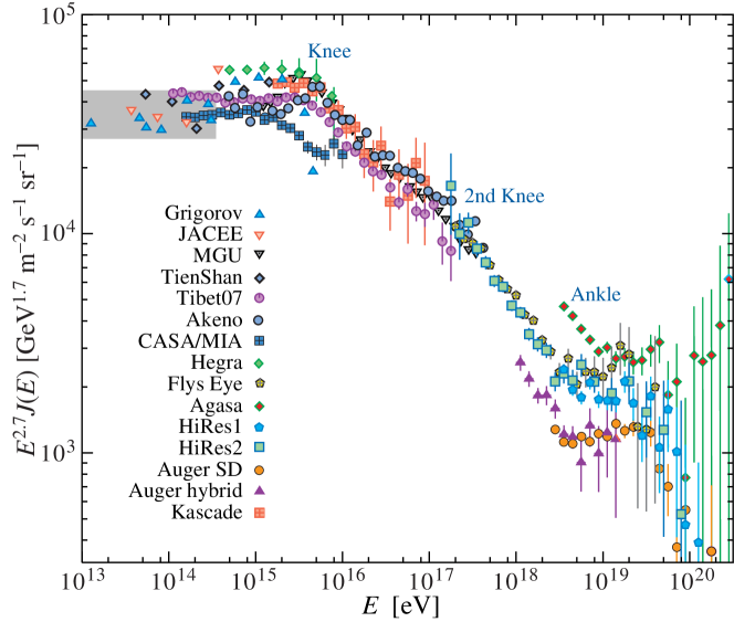
Figure 2: All-particle spectrum of cosmic rays. From Ref. [15].

A steepening of the spectrum ($\gamma\simeq 2.7\to 3.1$) at an energy of about $10^{6.5}$ GeV is known as the cosmic ray knee. Composition measurements in cosmic ray observatories indicate that this feature of the spectrum is composed of the subsequent fall-off of Galactic nuclear components with maximal energy $E/Z$ [16, 17, 18]. This scaling with atomic number $Z$ is expected for particle acceleration in a magnetically confining environment, which is only effective as long as the particle’s Larmor radius is smaller than the size of the accelerator. If this interpretation holds, the Galactic contribution in CRs can not extend much further than $10^{8}$ GeV, assuming iron ($Z=26$) as the heaviest component. However, the observational data at these energies is inconclusive and the end-point of Galactic CRs has not been pinned down so far. For a survey of spectral features at lower energies see [19].

The onset of an extragalactic contribution could be signaled by the so-called second knee – a further steepening ($\gamma\simeq 3.1\to 3.2$) of the spectrum at about $10^{8.7}$ GeV. Note that extragalactic CRs are subject to collisions with the interstellar medium during their propagation over cosmological distances. Depending on the initial chemical composition, these particle-specific interactions will be imprinted in the spectrum observed on Earth. It has been argued [20, 21] that an extragalactic proton population with a simple power-law injection spectrum may reproduce the spectrum above the second knee. In these models the flattening ($\gamma\simeq 3.2\to 2.7$) in the spectrum at around $10^{9.5}$ GeV – the so-called ankle – can be identified as a “dip” from $e^{+}e^{-}$ pair production together with a “pile-up” of protons from pion photoproduction. However, this feature relies on a proton dominance in extragalactic cosmic rays since heavier nuclei like oxygen or iron have different energy loss properties in the cosmic microwave background (CMB) and mixed compositions, in general will not reproduce the spectral features [22]. A cross-over at higher energies is also feasible: above the ankle the Larmor radius of a proton in the galactic magnetic field exceeds the size of the Galaxy and it is generally assumed that an extragalactic component dominates the spectrum at these energies [23]. Moreover, the galactic-extragalactic transition ought to be accompanied by the appearence of spectral features, e.g. two power-law contributions would naturally produce a flattening in the spectrum if the harder component dominates at lower energies. Hence, the ankle seems to be the natural candidate for this transition.

Shortly after the CMB was discovered [24], Greisen [25], Zatsepin, and Kuzmin [26] (GZK) pointed out that the relic photons make the universe opaque to CRs of sufficiently high energy. This occurs, for example, for protons with energies beyond the photopion production threshold,

$$E_{p\gamma_{\rm CMB}}^{\rm th}=\frac{m_{\pi}\,(m_{p}+m_{\pi}/2)}{\omega_{\rm CMB}}\approx 6.8\times 10^{10}\,\left(\frac{\omega_{\rm CMB}}{10^{-3}\leavevmode\nobreak\ {\rm eV}}\right)^{-1}\,\,{\rm GeV}\,,$$ (1)

where $m_{p}$ ($m_{\pi}$) denotes the proton (pion) mass and $\omega_{\rm CMB}\sim 10^{-3}$ eV is a typical CMB photon energy. After pion production, the proton (or perhaps, instead, a neutron) emerges with at least 50% of the incoming energy. This implies that the nucleon energy changes by an $e$-folding after a propagation distance $\lesssim(\sigma_{p\gamma}\,n_{\gamma}\,y_{\pi})^{-1}\sim 15$ Mpc. Here, $n_{\gamma}\approx 410$ cm^-3 is the number density of the CMB photons, $\sigma_{p\gamma}>0.1$ mb is the photopion production cross section, and $y_{\pi}$ is the average energy fraction (in the laboratory system) lost by a nucleon per interaction. For heavy nuclei, the giant dipole resonance (GDR) can be excited at similar total energies and hence, for example, iron nuclei do not survive fragmentation over comparable distances. Additionally, the survival probability for extremely high energy ($\approx 10^{11}$ GeV) $\gamma$-rays (propagating on magnetic fields $\gg 10^{-11}$ G) to a distance $d$, $p(>d)\approx\exp[-d/6.6\leavevmode\nobreak\ {\rm Mpc}]$, becomes less than $10^{-4}$ after traversing a distance of 50 Mpc. All in all, as our horizon shrinks dramatically for energies $\gtrsim 10^{11}$ GeV, one would expect a sudden suppression in the energy spectrum if the CR sources follow a cosmological distribution.

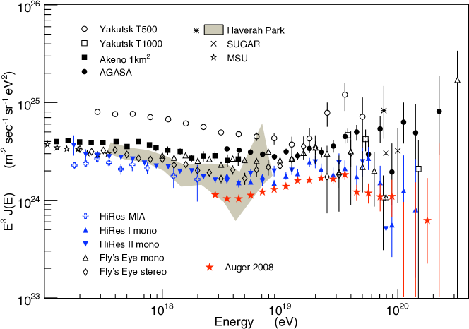
Figure 3: Comparison of flux measurements scaled by $E^{3}$. Only statistical errors are shown. Shown are the data of AGASA, Akeno, Auger, Fly’s Eye, Haverah Park, HiRes-MIA, HiRes Fly’s Eye, MSU, SUGAR, and Yakutsk. Yakutsk T500 (trigger 500) refers to the smaller sub-array of the experiment with 500m detector spacing and T1000 (trigger 1000) to the array with 1000m detector distance. In case several analyses of the same data set are available, only the most recent results are included in the plot. The shaded area, depicting the results of the analysis of the Haverah Park data, accounts for some systematic uncertainties by assuming extreme elemental compositions, either fully iron or proton dominated. The highest energy point (Fly’s Eye monocular observation) corresponds to the highest energy event. For sake of clarity, upper limits are not shown. The data of the MSU array are included to show the connection of the high-energy measurements to lower energy data covering the knee of the cosmic-ray spectrum. From Ref. [19].

At the beginning of summer 2002, in a pioneering paper Bahcall and Waxman [27] noted that the energy spectra of CRs reported by the AGASA, the Fly’s Eye, the Haverah Park, the HiRes, and the Yakutsk collaborations (see Fig. 3) are consistent with the expected GZK suppression at $\sim 3.5\sigma$ level according to the Fly’s Eye normalization, increasing up to $\sim 8\sigma$ if the selected normalization is that of Yakutsk. Five years later, the HiRes Collaboration reported a suppression of the CR flux above $E=[5.6\pm 0.5({\rm stat})\pm 0.9({\rm syst})]\times 10^{10}\leavevmode\nobreak\ {\rm GeV}$, with 5.3$\sigma$ significance [28]. The spectral index of the flux steepens from $2.81\pm 0.03$ to $5.1\pm 0.7$. The discovery of the GZK suppression has been confirmed by the Pierre Auger Collaboration, measuring $\gamma=2.69\pm 0.2({\rm stat})\pm 0.06({\rm syst})$ and $\gamma=4.2\pm 0.4({\rm stat})\pm 0.06({\rm syst})$ below and above $E=4.0\times 10^{10}\leavevmode\nobreak\ {\rm GeV}$, respectively (the systematic uncertainty in the energy determination is estimated as 22%) [29].

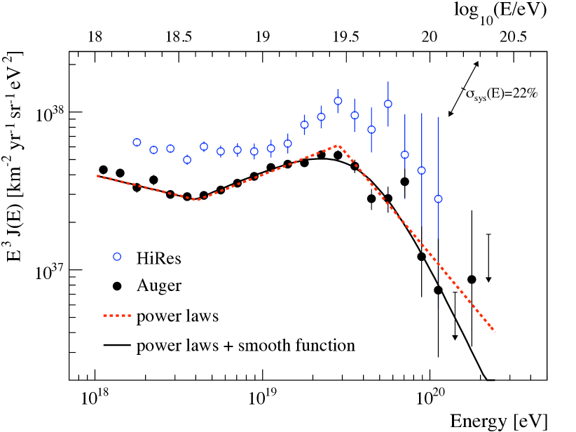
Figure 4: Combined spectrum from Auger (hybrid and SD events) and the stereo spectrum HiReS. The Auger systematic uncertainty of the flux scaled by $E^{3}$, due to the uncertainty of the energy scale of 22%, is indicated by arrows. The results of the two experiments are consistent within systematic uncertainties. From Ref. [30].

Last year, an updated Auger measurement of the energy spectrum was published [30], corresponding to a surface array exposure of $12,790\leavevmode\nobreak\ {\rm km}^{2}\leavevmode\nobreak\ {\rm sr\leavevmode\nobreak\ yr}$. This measurement, combining both hybrid and SD-only events, is shown in Fig. 4. The ankle feature and flux suppression are clearly visible. A broken power law fit to the spectrum shows that the break corresponding to the ankle is located at $\log_{10}(E/{\rm eV})=18.61\pm 0.01$ with $\gamma=3.26\pm 0.04$ before the break and $\gamma=2.59\pm 0.02$ after it. The break corresponding to the suppression is located at $\log_{10}(E/{\rm eV})=19.46\pm 0.03$. Compared to a power law extrapolation, the significance of the suppression is greater than $20\sigma$.

Primary species

Unfortunately, because of the highly indirect method of measurement, extracting precise information from EASs has proved to be exceedingly difficult. The most fundamental problem is that the first generations of particles in the cascade are subject to large inherent fluctuations and consequently this limits the event-by-event energy resolution of the experiments. In addition, the center-of-mass (c.m.) energy of the first few cascade steps is well beyond any reached in collider experiments. Therefore, one needs to rely on hadronic interaction models that attempt to extrapolate, using different mixtures of theory and phenomenology, our understanding of particle physics.

The longitudinal development has a well defined maximum, usually referred to as $X_{\rm max}$, which increases with primary energy as more cascade generations are required to degrade the secondary particle energies. Evaluating $X_{\rm max}$ is a fundamental part of many of the composition studies done by detecting air showers. For showers of a given total energy $E$, heavier nuclei have smaller $X_{\rm max}$ because the shower is already subdivided into $A$ nucleons when it enters the atmosphere. The average depth of maximum $\langle X_{\rm max}\rangle$ scales approximately as $\ln(E/A)$ [31]. Therefore, since $\langle X_{\rm max}\rangle$ can be determined directly from the longitudinal shower profiles measured with a fluorescence detector, the composition can be extracted after estimating $E$ from the total fluorescence yield. Indeed, the parameter often measured is $D_{10}$, the rate of change of $\langle X_{\rm max}\rangle$ per decade of energy.

Photons penetrate quite deeply into the atmosphere due to decreased secondary multiplicities and suppression of cross sections by the Landau-Pomeranchuk-Migdal (LPM) effect [32, 33]. Indeed, it is rather easier to distinguish photons from protons and iron than protons and iron are to distinguish from one another. For example, at $10^{10}\leavevmode\nobreak\ {\rm GeV}$, the $\langle X_{\rm max}\rangle$ for a photon is about 1000 g/cm², while for protons and iron the numbers are 800 g/cm² and 700 g/cm², respectively.

Searches for photon primaries have been conducted using both the surface and fluorescence istruments of Auger. While analysis of the fluorescence data exploits the direct view of shower development, analysis of data from the surface detector relies on measurement of quantities which are indirectly related to the $X_{\rm max}$, such as the signal risetime at 1000 m from the shower core and the curvature of the shower front. Presently, the 95% CL upper limits on the fraction of CR photons above $2,\ 3,\ 5,\ 10,\ 20,$ and $40\times 10^{9}\leavevmode\nobreak\ {\rm GeV}$ are $3.8\%,2.4\%,3.5\%,2.0\%,\ 5.1\%,$ and $31\%,$ respectively. Further details on the analysis procedures can be found in [34, 35, 36]. In Fig. 5 these upper limits are compared with predictions of the cosmogenic photon flux.

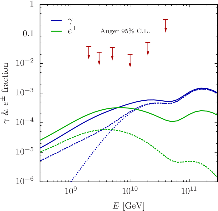
Figure 5: Upper limits on the photon fraction reported by the Pierre Auger Collaboration. A prediction for the cosmogenic photon flux is also shown for comparison (details on the calculation are given Sec. 0.2.5) The color and line coding is the same as the one in Fig. 37. This figure is courtesy of Markus Ahlers.

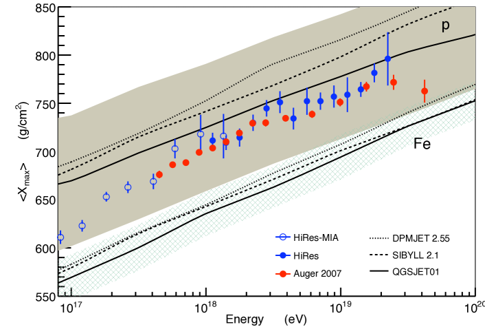
Figure 6: The compilation of fluorescence-based measurements of the mean $X_{\rm max}$ of various experiments is compared with predictions from EAS simulations using three event generators of hadronic interactions (sibyll, qgsjet, and dpmjet). The qgsjet predictions on the shower-to-shower fluctuations of the depth of maximum are indicated by the shaded (cross-hatched) area for proton (iron) primaries. From Ref. [19].

In Fig. 6 we show the variation of $\langle X_{\rm max}\rangle$ with primary energy as measured by several experiments. Interpreting the results of these measurements relies on comparison to the predictions of high energy hadronic interaction models. As one can see in Fig. 6, there is considerable variation in predictions among the different interaction models. For $1.6\times 10^{9}\leavevmode\nobreak\ {\rm GeV}<E<6.3\times 10^{10}\leavevmode\nobreak\ {\rm GeV}$, the HiRes data are consistent with a constant elongation rate $d\langle X_{\rm max}\rangle/d(\log(E))=47.9\pm 6.0({\rm stat})\pm 3.2({\rm sys})\leavevmode\nobreak\ {\rm g}/{\rm cm}^{2}/{\rm decade}$ [37]. The inference from the HiRes data is therefore a change in cosmic ray composition, from heavy nuclei to protons, at $E\sim 10^{8.6}$ GeV [38]. This is an order of magnitude lower in energy than the previous crossover deduced from the Fly’s Eye data [39]. On the other hand, Auger measurements, interpreted with current hadronic interaction models, seem to favor a mixed (protons + nuclei) composition at energies above $10^{8.6}\leavevmode\nobreak\ {\rm GeV}$ [40]. However, uncertainties in the extrapolation of the proton-air interaction – cross section [41] and elasticity and multiplicity of secondaries [42] – from accelerator measurements to the high energies characteristic for air showers are large enough to undermine any definite conclusion on the chemical composition.

Distribution of arrival directions

There exists “lore” that convinces us that the highest energy CRs observed should exhibit trajectories which are relatively unperturbed by galactic and intergalactic magnetic fields. Hence, it is natural to wonder whether anisotropy begins to emerge at these high energies. Furthermore, if the observed flux suppression is the GZK effect, there is necessarily some distance, O(100 Mpc), beyond which cosmic rays with energies near $10^{11}$ GeV will not be seen. Since the matter density within about 100 Mpc is not isotropic, this compounds the potential for anisotropy to emerge in the UHECR sample. On the one hand, if the distribution of arrival directions exhibits a large-scale anisotropy, this could indicate whether or not certain classes of sources are associated with large-scale structures (such as the Galactic plane or the Galactic halo). On the other hand, if cosmic rays cluster within a small angular region or show directional alignment with powerful compact objects, one might be able to associate them with isolated sources in the sky.

CR air shower detectors which experience stable operation over a period of a year or more can have a uniform exposure in right ascension, $\alpha$. A traditional technique to search for large-scale anisotropies is then to fit the right ascension distribution of events to a sine wave with period $2\pi/m$ ($m^{\rm th}$ harmonic) to determine the components ($x,y$) of the Rayleigh vector [43]

$$x=\frac{2}{{\cal N}}\sum_{i=1}^{N}\,w_{i}\,\cos(m\,\alpha_{i})\,,\,\,\,\,\,y=\frac{2}{{\cal N}}\sum_{i=1}^{N}\,w_{i}\,\,\,\sin(m\,\alpha_{i})\,,$$ (2)

where the sum runs over the number of $N$ events in the considered energy range, ${\cal N}=\sum_{i=1}^{N}w_{i}$ is the normalization factor, and the weights, $w_{i}=\omega^{-1}(\delta_{i})$, are the reciprocal of the relative exposure, $\omega$, given as a function of the declination, $\delta_{i}$ [44]. The $m^{\rm th}$ harmonic amplitude of $N$ measurements of $\alpha_{i}$ is given by the Rayleigh vector length ${\cal R}\leavevmode\nobreak\ =\leavevmode\nobreak\ (x^{2}\leavevmode\nobreak\ +\leavevmode\nobreak\ y^{2})^{1/2}$, and the phase is $\varphi={\rm arctan}(y/x)$. The expected length of such a vector for values randomly sampled from a uniform phase distribution is ${\cal R}_{0}\leavevmode\nobreak\ =\leavevmode\nobreak\ 2/\sqrt{{\cal N}}$. The chance probability of obtaining an amplitude with length larger than that measured is $p(\geq\leavevmode\nobreak\ {\cal R})\leavevmode\nobreak\ =\leavevmode\nobreak\ e^{-k_{0}},$ where $k_{0}\leavevmode\nobreak\ =\leavevmode\nobreak\ {\cal R}^{2}/{\cal R}_{0}^{2}.$ To give a specific example, a vector of length $k_{0}\leavevmode\nobreak\ \geq\leavevmode\nobreak\ 6.6$ would be required to claim an observation whose probability of arising from random fluctuation was 0.0013 (a “$3\sigma$” result) [45]. For a given CL, upper limits on the amplitude can be derived using a distribution drawn from a population characterized by an anisotropy of unknown amplitude and phase

$${\rm CL}=\sqrt{\frac{2}{\pi}}\frac{1}{I_{0}({\cal R}^{2}/4\sigma^{2})}\int_{0}^{{\cal R}_{UL}}\frac{ds}{\sigma}\,I_{0}\bigg{(}\frac{{\cal R}s}{\sigma^{2}}\bigg{)}\,\exp{\bigg{(}-\frac{s^{2}+{\cal R}^{2}/2}{2\sigma^{2}}\bigg{)}},$$ (3)

where $I_{0}$ is the modified Bessel function of the first kind with order zero and $\sigma=\sqrt{2/\mathcal{N}}$ [43].

The first harmonic amplitude of the CR right ascension distribution can be directly related to the amplitude $\alpha_{d}$ of a dipolar distribution of the form $J(\alpha,\delta)=J_{0}(1+\alpha_{d}\ \hat{d}\cdot\hat{u})$, where $\hat{u}$ and $\hat{d}$ respectively denote the unit vector in the direction of an arrival direction and in the direction of the dipole. Setting $m=1$, we can rewrite $x$, $y$ and $\mathcal{N}$ as:

$$x = \frac{2}{\mathcal{N}}\int_{\delta_{min}}^{\delta_{max}}d\delta\int_{0}^{2\pi}d\alpha\cos\delta\ J(\alpha,\delta)\ \omega(\delta)\cos\alpha,$$

$$y = \frac{2}{\mathcal{N}}\int_{\delta_{min}}^{\delta_{max}}d\delta\int_{0}^{2\pi}d\alpha\cos\delta\ J(\alpha,\delta)\ \omega(\delta)\sin\alpha,$$ (4)

$$\mathcal{N} = \int_{\delta_{min}}^{\delta_{max}}d\delta\int_{0}^{2\pi}d\alpha\cos\delta\ J(\alpha,\delta)\ \omega(\delta)\,.$$

In (4) we have neglected the small dependence on right ascension in the exposure. Next, we write the angular dependence in $J(\alpha,\delta)$ as $\hat{d}\cdot\hat{u}=\cos\delta\cos\delta_{0}\cos(\alpha-\alpha_{0})+\sin\delta\sin\delta_{0}$, where $\alpha_{0}$ and $\delta_{0}$ are the right ascension and declination of the apparent origin of the dipole, respectively. Performing the $\alpha$ integration in (4) it follows that

$${\cal R}=\left|\frac{Ad_{\perp}}{1+Bd_{\parallel}}\right|$$ (5)

where

$$A=\frac{\int d\delta\,\omega(\delta)\cos^{2}\delta}{\int d\delta\,\omega(\delta)\cos\delta}\,,\hskip 28.45274ptB=\frac{\int d\delta\,\omega(\delta)\cos\delta\sin\delta}{\int d\delta\,\omega(\delta)\cos\delta}\,,$$

$d_{\parallel}=\alpha_{d}\sin{\delta_{0}}$ is the component of the dipole along the Earth rotation axis, and $d_{\perp}=\alpha_{d}\cos{\delta_{0}}$ is the component in the equatorial plane [46]. The coefficients $A$ and $B$ can be estimated from the data as the mean values of the cosine and the sine of the event declinations. For example, for the Auger data sample we have $A=\left<\cos{\delta}\right>\simeq 0.78$ and $B=\left<\sin{\delta}\right>\simeq-0.45$. For a dipole amplitude $\alpha_{d}$, the measured amplitude of the first harmonic in right ascension ${\cal R}$ thus depends on the region of the sky observed, which is essentially a function of the latitude of the observatory $\ell_{\rm site}$, and the range of zenith angles considered. In the case of a small $Bd_{\parallel}$ factor, the dipole component in the equatorial plane $d_{\perp}$ is obtained as $d_{\perp}\simeq{\cal R}/\langle\cos{\delta}\rangle$. The phase $\varphi$ corresponds to the right ascension of the dipole direction $\alpha_{0}$. For a fixed number of arrival directions, the RMS error in the amplitude, $\Delta\alpha_{d}\approx 1.5N^{-1/2},$ has little dependence on the amplitude [44].

In Fig. 7 we show upper limits and measurements of $d_{\perp}$ from various experiments together with some predictions from UHECR models of both galactic and extragalactic origin. The AGASA Collaboration reported a correlation of the CR arrival directions to the Galactic plane at the $4\sigma$ level [49]. The energy bin width which gives the maximum $k_{0}$-value corresponds to the region $10^{8.9}$ GeV – $10^{9.3}$ GeV where $k_{0}=11.1,$ yielding a chance probability of $p(\geq\leavevmode\nobreak\ {\cal R}_{{}_{E\sim{\rm EeV}}}^{{}^{\rm AGASA}})\approx 1.5\times 10^{-5}.$ The recent results reported by the Pierre Auger Collaboration are inconsistent with those reproted by the AGASA Collaboration [48]. If the galactic/extragalactic transition occurs at the ankle, UHECRs at $10^{9}$ GeV are predominantly of galactic origin and their escape from the Galaxy by diffusion and drift motions are expected to induce a modulation in this energy range. These predictions depend on the assumed galactic magnetic field model as well as on the source distribution and the composition of the UHECRs. Two alternative models are displayed in Fig. 7, corresponding to different geometries of the halo magnetic fields [50]. The bounds reported by the Pierre Auger Collaboration already exclude the particular model with an antisymmetric halo magnetic field ($A$) and are starting to become sensitive to the predictions of the model with a symmetric field ($S$). The predictions shown in Fig. 7 are based on the assumption of predominantly heavy composition in the galactic component [51]. Scenarios in which galactic protons dominate at $10^{9}$ GeV would typically predict a larger anisotropy. Alternatively, if the structure of the magnetic fields in the halo is such that the turbulent component dominates over the regular one, purely diffusion motions may confine light elements of galactic origin up to $\simeq 10^{9}$ GeV, and may induce an ankle-like feature at higher energy due to the longer confinement of heavier elements [52]. Typical signatures of such a scenario in terms of large scale anisotropies are also shown in Fig. 7 (dotted line). The corresponding amplitudes are challenged by the current sensitivity of Auger. On the other hand, if the transition is taking place at lower energies, say around the second knee, UHECRs above $10^{9}$ GeV are dominantly of extragalactic origin and their large scale distribution could be influenced by the relative motion of the observer with respect to the frame of the sources. If the frame in which the UHECR distribution is isotropic coincides with the CMB rest frame, a small anisotropy is expected due to the Compton-Getting effect [53]. Neglecting the effects of the galactic magnetic field, this anisotropy would be a dipolar pattern pointing in the direction $\alpha_{0}\simeq 168^{\circ}$ with an amplitude of about 0.6% [54], close to the upper limits set by the Pierre Auger Collaboration. The statistics required to detect an amplitude of 0.6% at 99% CL is $\simeq 3$ times the published Auger sample [48].

The right harmonic analyses are completely blind to intensity variations which depend only on declination. Combining anisotropy searches in $\alpha$ over a range of declinations could dilute the results, since significant but out of phase Rayleigh vectors from different declination bands can cancel each other out. An unambiguous interpretation of anisotropy data requires two ingredients: exposure to the full celestial sphere and analysis in terms of both celestial coordinates [44].

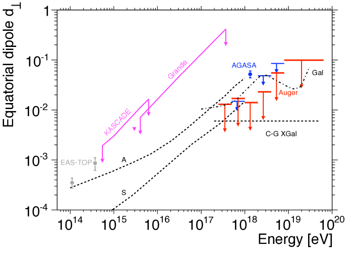
Figure 7: Upper limits on the anisotropy amplitude of first harmonic as a function of energy from Auger, EAS-TOP, AGASA, KASCADE and KASCADE-Grande experiments. Also shown are the predictions up to 1 EeV from two different galactic magnetic field models with different symmetries ($A$ and $S$), the predictions for a purely galactic origin of UHECRs up to a few times $10^{10}\,$ GeV ($Gal$), and the expectations from the Compton-Getting effect for an extragalactic component isotropic in the CMB rest frame ($C$-$G\,XGal$). Below 1 EeV, due to variations of the event counting rate arising from atmospheric effects, the Pierre Auger Collaboration adopted the East/West method [47], which is two times less efficient but doesn’t require correction for trigger efficiency. From Ref. [48]

.

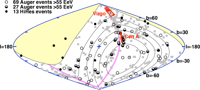
Figure 8: Correlation of the arrival directions of UHECR with AGNs from the VCV catalog. The shaded part of the sky is not visible by Auger. The gray squares are the AGNs within $z$ less than 0.018. The Auger events are shown with circles. The first 27 events are half filled. The 13 HiRes events are shown with black dots. The thin lines show the six regions of the sky to which Auger has equal exposure. The wide gray line is the supergalactic plane. From Ref. [5].

One way to increase the chance of success in finding out the sources of UHECRs is to check for correlations between CR arrival directions and known candidate astrophysical objects. To calculate a meaningful statistical significance in such an analysis, it is important to define the search procedure a priori in order to ensure it is not inadvertently devised especially to suit the particular data set after having studied it. With the aim of avoiding accidental bias on the number of trials performed in selecting the cuts, the Auger anisotropy analysis scheme followed a pre-defined process. First an exploratory data sample was employed for comparison with various source catalogs and for tests of various cut choices. The results of this exploratory period were then used to design prescriptions to be applied to subsequently gathered data.

Based on the results of scanning an exposure of $4,390\leavevmode\nobreak\ {\rm km}^{2}$ sr yr, a prescription was designed to test the correlation of events having energies $E>5.5\times 10^{10}$ GeV with objects in the Veron-Cetty & Veron (VCV) catalog of Active Galactic Nuclei (AGNs). The prescription called for a search of $3.1^{\circ}$ windows around catalog objects with redshifts $z<0.0018$. The significance threshold set in the prescription was met in 2007, when the exposure more than doubled and the total number of events reached 27, with 9 of the 13 events in the post-prescription sample correlating [56, 55]. For a sample of 13 events from an isotropic distribution, the probability that 9 or more correlate by chance with an object in the AGN catalogue (subject to cuts on the exposure weighted fraction of the sky within the opening angles and the redshift) is less than 1%. This corresponds to roughly a $2.5\sigma$ effect. In the summer of 2008, the HiRes Collaboration applied the Auger prescription to their data set and found no significant correlation [57]. One has to exercise caution when comparing results of different experiments with potentially different energy scales, since the analysis involves placing an energy cut on a steeply falling spectrum. More recently, the Pierre Auger Collaboration published an update on the correlation results from an exposure of $20,370\leavevmode\nobreak\ {\rm km}^{2}$ sr yr (collected over 6 yr but equivalent to 2.9 yr of the nominal exposure/yr of the full Auger), which contains 69 events with $E>5.5\times 10^{10}$ GeV [58]. A skymap showing the locations of all these events is displayed in Fig. 8. For a physical signal one expects the significance to increase as more data are gathered. In this study, however, the significance has not increased. A $3\sigma$ effect is not neccesarily cause for excitement; of every 100 experiments, you expect about one $3\sigma$ effect. Traditionally, in particle physics there is an unwritten $5\sigma$ rule for “discovery.” One should keep in mind though that in the case of CR physics we do not have the luxury of controlling the luminosity.

A number of other interesting observations are described in [58], including comparisons with other catalogs as well as a specific search around the region of the nearest active galaxy, Centaurus A (Cen A). It is important to keep in mind that these are all a posteriori studies, so one cannot use them to determine a confidence level for anisotropy as the number of trials is unknown. A compelling concentration of events in the region around the direction of Cen A has been observed. As one can see in Fig. 9, the maximum departure from isotropy occurs for a ring of $18^{\circ}$ around the object, in which 13 events are observed compared to an expectation of 3.2 from isotropy. There are no events coming from less than $18^{\circ}$ around M87, which is almost 5 times more distant than Cen A and lies at the core of the Virgo cluster. As shown in Fig. 8 the Auger exposure is 3 times smaller for M87 than for Cen A. Using these two rough numbers and assuming equal luminosity, one expects 75 times fewer events from M87 than from Cen A. Hence, the lack of events in this region is not completely unexpected.

The Centaurus cluster lies 45 Mpc behind Cen A. An interesting question then is whether some of the events in the $18^{\circ}$ circle could come from the Centaurus cluster rather than from Cen A. This does not appear likely because the Centaurus cluster is farther away than the Virgo cluster and for comparablel CR luminosities one would expect a small fraction of events coming from Virgo. Furthermore, the events emitted by Cen A and deflected by magnetic fields could still register as a correlation due to the overdense AGN population lying behind Cen A, resulting in a spurious signal [59].

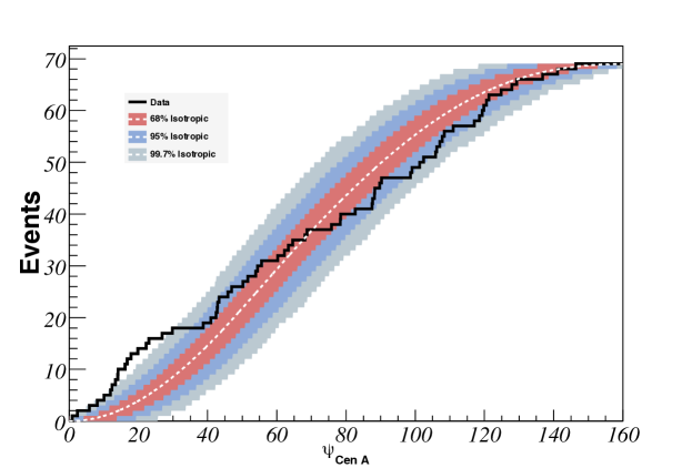
Figure 9: Cumulative number of events with $E\geq 55$ EeV as a function of angular distance from the direction of Cen A. The bands correspond to the 68%, 95%, and 99.7% dispersion expected for an isotropic flux. From Ref. [58].

In summary, the inaugural years of data taking at the Pierre Auger Observatory have yielded a large, high-quality data sample. The enormous area covered by the surface array together with an excellent fluorescence system and hybrid detection techniques have provided us with large statistics, good energy resolution, and solid control of systematic uncertainties. Presently, Auger is collecting some $7,000\leavevmode\nobreak\ {\rm km}^{2}\leavevmode\nobreak\ {\rm sr}\leavevmode\nobreak\ {\rm yr}$ of exposure each year, and is expected to run for 2 more decades. New detector systems are being deployed, which will lower the energy detection threshold down to $10^{8}$ GeV. An experimental radio detection program is also co-located with the observatory and shows promising results. As always, the development of new analysis techniques is ongoing, and interesting new results can be expected.

0.2.2 Origin of ultrahigh energy cosmic rays

It is most likely that the bulk of the cosmic radiation is a result of some very general magneto-hydrodynamic (MHD) phenomenon in space which transfers kinetic or magnetic energy into cosmic ray energy. The details of the acceleration process and the maximum attainable energy depend on the particular physical situation under consideration. There are basically two types of mechanism that one might invoke. The first type assumes the particles are accelerated directly to very high energy (VHE) by an extended electric field [60]. This idea can be traced back to the early 1930’s when Swann [61] pointed out that betatron acceleration may take place in the increasing magnetic field of a sunspot. These so-called “one-shot” mechanisms have been worked out in greatest detail, and the electric field in question is now generally associated with the rapid rotation of small, highly magnetized objects such as neutron stars (pulsars) or AGNs. Electric field acceleration has the advantage of being fast, but suffers from the circumstance that the acceleration occurs in astrophysical sites of very high energy density, where new opportunities for energy loss exist. Moreover, it is usually not obvious how to obtain the observed power law spectrum in a natural way, and so this kind of mechanism is not widely favored these days. The second type of process is often referred to as statistical acceleration, because particles gain energy gradually by numerous encounters with moving magnetized plasmas. These kinds of models were mostly pioneered by Fermi [62]. In this case the $E^{-2}$ spectrum emerges very convincingly. However, the process of acceleration is slow, and it is hard to keep the particles confined within the Fermi engine. In this section we first provide a summary of statistical acceleration based on the simplified version given in Ref. [63]. For a more detailed and rigorous discussion, the reader is referred to [64]. After reviewing statistical acceleration, we turn to the issue of the maximum achievable energy within diffuse shock acceleration and explore the viability of some proposed UHECR sources.

Fermi acceleration at shock waves

In his original analysis, Fermi [62] considered the scattering of CRs on moving magnetized clouds. The right panel of Fig. 10 shows a sketch of these encounters. Consider a CR entering into a single cloud with energy $E_{i}$ and incident angle $\theta_{i}$ with the cloud’s direction undergoing diffuse scattering on the irregularities in the magnetic field. After diffusing inside the cloud, the particle’s average motion coincides with that of the gas cloud. The energy gain by the particle, which emerges at an angle $\theta_{f}$ with energy $E_{f}$, can be obtained by applying Lorentz transformations between the laboratory frame (unprimed) and the cloud frame (primed). In the rest frame of the moving cloud, the CR particle has a total initial energy

$$E_{i}^{\prime}=\Gamma_{\rm cloud}\,E_{i}\,(1-\beta_{\rm cloud}\,\cos\theta_{i})\,,$$ (6)

where $\Gamma_{\rm cloud}$ and $\beta_{\rm cloud}=V_{\rm cloud}/c$ are the Lorentz factor and velocity of the cloud in units of the speed of light, respectively. In the frame of the cloud we expect no change in energy ($E_{i}^{\prime}=E_{f}^{\prime}$), because all the scatterings inside the cloud are due only to motion in the magnetic field (so-called collisionless scattering). There is elastic scattering between the CR and the cloud as a whole, which is much more massive than the CR. Transforming to the laboratory frame we find that the energy of the particle after its encounter with the cloud is

$$E_{f}=\Gamma_{\rm cloud}\,E_{f}^{\prime}\,(1+\beta_{\rm cloud}\cos\theta_{f})\,.$$ (7)

The fractional energy change in the laboratory frame is then

$$\frac{\Delta E}{E}=\frac{E_{f}-E_{i}}{E_{i}}=\frac{1-\beta_{\rm cloud}\cos\theta_{i}+\beta_{\rm cloud}\cos\theta_{f}-\beta_{\rm cloud}^{2}\cos\theta_{i}\cos\theta_{f}}{1-\beta_{\rm cloud}^{2}}-1\,.$$ (8)

Inside the cloud the CR direction becomes randomized and so $\langle\cos\theta_{f}\rangle=0.$ The collisionless scattered particle will gain energy in a head-on collision ($\theta_{i}>\pi/2$) and lose energy by tail-end ($\theta_{i}<\pi/2$) scattering. The net increase of its energy is a statistical effect. The average value of $\cos\theta_{i}$ depends on the relative velocity between the cloud and the particle. The probability $P$ per unit solid angle $\Omega$ of having a collision at angle $\theta_{i}$ is proportional to $(v-V_{\rm cloud}\cos\theta_{i})$, where $v$ is the CR speed. In the ultrarelativistic limit, i.e., $v\sim c$ (as seen in the laboratory frame),

$$\frac{dP}{d\Omega_{i}}\propto(1-\beta_{\rm cloud}\cos\theta_{i})\,,$$ (9)

so

$$\langle\cos\theta_{i}\rangle=-\frac{\beta_{\rm cloud}}{3}\,.$$ (10)

Now, inserting Eq. (10) into Eq.(8), one obtains for $\beta_{\rm cloud}\ll 1$,

$$\frac{\langle\Delta E\rangle}{E}=\frac{1+\beta_{\rm cloud}^{2}/3}{1-\beta_{\rm cloud}^{2}}-1\approx\frac{4}{3}\,\beta_{\rm cloud}^{2}\,.$$ (11)

Note that $\langle\Delta E\rangle/E\propto\beta_{\rm cloud}^{2}$, so even though the average magnetic field may vanish, there can still be a net transfer of the macroscopic kinetic energy from the moving cloud to the particle. However, the average energy gain is very small, because $\beta_{\rm cloud}^{2}\ll 1$. This acceleration process is very similar to a thermodynamical system of two gases, which tries to come into thermal equilibrium [66]. Correspondingly, the spectrum of CRs should follow a thermal spectrum which might be in conflict with the observed power-law.

A more efficient acceleration may occur in the vicinity of plasma shocks occurring in astrophysical environments [67, 68]. Suppose that a strong (nonrelativistic) shock wave propagates through the plasma as sketched in the left panel of Fig. 10. Then, in the rest frame of the shock the conservation relations imply that the upstream velocity $u_{\rm up}$ (ahead of the shock) is much higher than the downstream velocity $u_{\rm down}$ (behind the shock). The compression ratio $r=u_{\text{up}}/u_{\text{down}}=n_{\text{down}}/n_{\text{up}}$ can be determined by requiring continuity of particle number, momentum, and energy across the shock; here $n_{\text{up}}$ ($n_{\text{down}}$) is the particle density of the upstream (downstream) plasma. For an ideal gas the compression ratio can be related to the specific heat ratio and the Mach number of the shock. For highly supersonic shocks, $r=4$ [64]. Therefore, in the primed frame stationary with respect to the shock, the upstream flow approaches with speed $u_{\rm up}=\beta_{\rm up}c=4\beta c/3$ and the downstream flow recedes with speed $u_{\rm down}=\beta_{\rm down}c=\beta c/3$. When measured in the stationary upstream frame, the quantity $u=u_{\rm up}-u_{\rm down}=\beta c$ is the speed of the shocked fluid and $u_{\rm up}=\beta_{\rm shock}$ is the speed of the shock. Hence, because of the converging flow – whichever side of the shock you are on, if you are moving with the plasma, the plasma on the other side of the shock is approaching you with velocity $u$ – to first order there are only head-on collisions for particles crossing the shock front. The acceleration process, although stochastic, always leads to a gain in energy. In order to work out the energy gain per shock crossing, we can visualize magnetic irregularities on either side of the shock as clouds of magnetized plasma of Fermi’s original theory. By considering the rate at which CRs cross the shock from downstream to upstream, and upstream to downstream, one finds $\langle\cos\theta_{i}\rangle=-2/3$ and $\langle\cos\theta_{f}\rangle=2/3$. Hence, Eq. (8) can be generalized to

$${\langle\Delta E\rangle\over E}\simeq{4\over 3}\beta=\frac{4}{3}\frac{u_{\rm up}-u_{\rm down}}{c}.$$ (12)

Note this is first order in $\beta=u/c$, and is therefore more efficient than Fermi’s original mechanism.

An attractive feature of Fermi acceleration is its prediction of a power-law flux of CRs. Consider a test-particle with momentum $p$ in the rest frame of the upstream fluid (see Fig. 10). The particle’s momentum distribution is isotropic in the fluid rest frame. For pitch angles $\pi/2<\theta_{i}<\pi$ relative to the shock velocity vector (see Fig. 10) the particle enters the downstream region and has on average the relative momentum $p[1+2(\beta_{\rm up}-\beta_{\rm down})/3]$. Subsequent diffusion in the downstream region ‘re-isotropizes’ the particle’s momentum distribution in the fluid rest frame. As the particle diffuses back into the upstream region (for pitch angles $0<\theta_{f}<\pi/2$) it has gained an average momentum of $\langle\Delta p\rangle/p\simeq 4(\beta_{\text{up}}-\beta_{\text{down}})/3$. This means that the momentum gain of a particle per time is proportional to its momentum,

$$\dot{p}=p/t_{\text{gain}}\,.$$ (13)

On the other hand, the loss of particles from the acceleration region is proportional to their number,

$$\dot{N}=-N/t_{\text{loss}}\,.$$ (14)

Therefore, taking the ratio (13)/(14) we first obtain

$$dN/dp=-\alpha N/p\,,$$ (15)

and after integration $N(p)\propto p^{-\alpha},$ with $\alpha=t_{\text{gain}}/t_{\text{loss}}$. If the acceleration cycle across the shock takes the time $\Delta t$ we have already identified $\Delta t/t_{\text{gain}}=\langle\Delta p\rangle/p\simeq 4(\beta_{\text{up}}-\beta_{\text{down}})/3$. For the loss of relativistic particles one finds $\Delta t/t_{\text{loss}}\simeq 4\beta_{\text{up}}$. Therefore, $\alpha\simeq 3\beta_{\text{up}}/(\beta_{\text{up}}-\beta_{\text{down}})=3r/(r-1)$, yielding $\alpha\simeq 4$ for highly supersonic shocks and $\alpha>4$ otherwise. The energy spectrum $N(E)\propto E^{-\gamma}$ is related to the momentum spectrum by ${\rm d}EN(E)=4\pi p^{2}{\rm d}pN(p)$ and hence $\gamma=\alpha-2\gtrsim 2$. The steeply falling spectrum of CRs with $\gamma\simeq 3$ seems to disfavor supersonic plasma shocks. However, for the comparison of these injection spectra with the flux of CRs observed on Earth, one has to consider particle interactions in the source and in the interstellar medium. This can have a great impact on the shape, as we will discuss in Secs. 0.2.4 and 0.2.5.

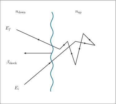
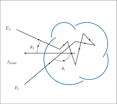
Figure 10: A sketch of 1st and 2nd order Fermi acceleration by scattering off plasma shocks (right) and magnetic clouds (left), respectively. From Ref. [65].

In general, the maximum attainable energy of Fermi’s mechanism is determined by the time scale over which particles are able to interact with the plasma. For the efficiency of a “cosmic cyclotron” particles have to be confined in the accelerator by its magnetic field $B$ over a sufficiently long time scale compared to the characteristic cycle time. The Larmor radius of a particle with charge $Ze$ increases with its energy $E$ according to

$$r_{L} = \sqrt{\frac{1}{4\pi\alpha}}\frac{E}{ZeB}$$ (16)

$$= \frac{1.1}{Z}\left(\frac{E}{\text{EeV}}\right)\left(\frac{B}{\mu\text{G}}\right)^{-1}\,{\rm kpc}\,.$$

The particle’s energy is limited as its Larmor radius approaches the characteristic radial size $R_{\text{source}}$ of the source

$$E_{\text{max}}\simeq Z\left(\frac{B}{\mu\text{G}}\right)\left(\frac{R_{\text{source}}}{\text{kpc}}\right)\,\times 10^{9}\leavevmode\nobreak\ {\rm GeV}\,.$$ (17)

This limitation in energy is conveniently visualized by the ‘Hillas plot’ [60] shown in Fig. 11 where the characteristic magnetic field $B$ of candidate cosmic accelerators is plotted against their characteristic size $R$. It is important to stress that in some cases the acceleration region itself only exists for a limited period of time; for example, supernovae shock waves dissipate after about $10^{4}$ yr. In such a case, Eq. (17) would have to be modifed accordingly. Otherwise, if the plasma disturbances persist for much longer periods, the maximum energy may be limited by an increased likelihood of escape from the region. A look at Fig. 11 reveals that the number of sources for the extremely high energy CRs around $10^{12}$ GeV is very sparse. For protons, only radio galaxy lobes and clusters of galaxies seem to be plausible candidates. For nuclei, terminal shocks of galactic superwinds originating in the metally-rich starburst galaxies are potential sources [69]. Exceptions may occur for sources which move relativistically in the host-galaxy frame, in particular jets from AGNs and gamma-ray bursts (GRBs). In this case the maximal energy might be increased due to a Doppler boost by a factor $\sim 30$ or $\sim 1000$, respectively.

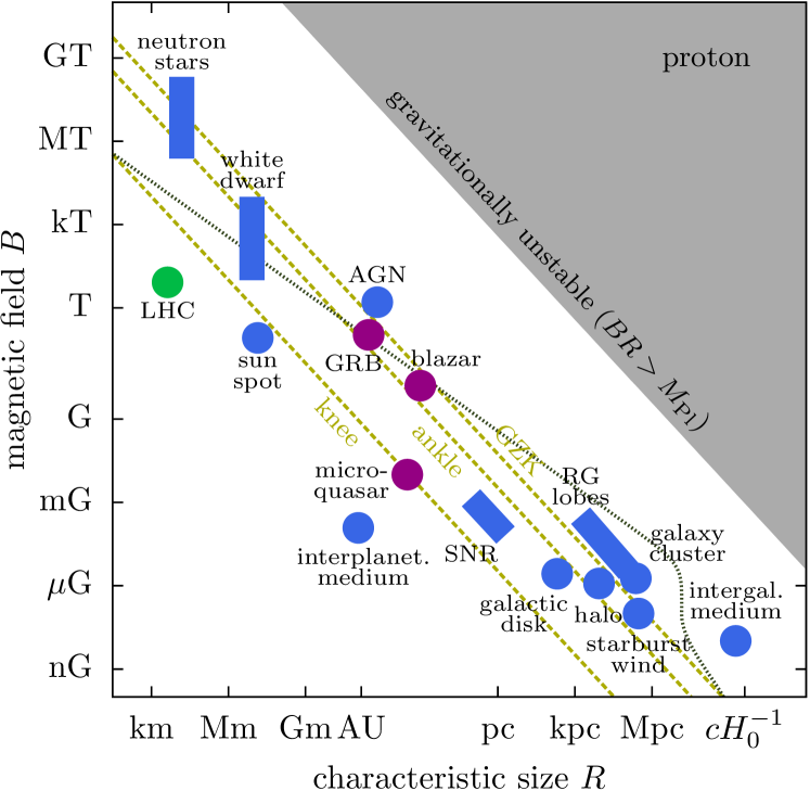
Figure 11: The “Hillas plot” for various CR source candidates (blue areas). Also shown are jet-frame parameters for blazers, gamma-ray bursts, and microquasars (purple areas). The corresponding point for the LHC beam is also shown. The red dashed lines show the lower limit for accelerators of protons at the CR knee ($\sim 10^{6.5}$ GeV), CR ankle ($\sim 10^{9.5}$ GeV) and the GZK suppression ($\sim 10^{10.6}$ GeV). The dotted gray line is the upper limit from synchrotron losses and proton interactions in the cosmic photon background ($R\gg 1$ Mpc). The grey area corresponds to astrophysical environments with extremely large magnetic field energy that would be gravitationally unstable. From Ref. [65].

For an extensive discussion on the potential CR-emitting-sources shown in Fig. 11, see e.g. [70]. Two of the most attractive examples are discussed next.

AGNs

AGNs are composed of an accretion disk around a central super-massive black hole and are sometimes associated with jets terminating in lobes which can be detected in radio. One can classify these objects into two categories: radio-quiet AGN with no prominent radio emission or jets and radio-loud objects presenting jets.

Fanaroff-Riley II (FRII) galaxies [71] are the largest known dissipative objects (non-thermal sources) in the cosmos. Localized regions of intense synchrotron emission, known as “hot spots,” are observed within their lobes. These regions are presumably produced when the bulk kinetic energy of the jets ejected by a central active nucleus is reconverted into relativistic particles and turbulent fields at a “working surface” in the head of the jets [72]. Specifically, the speed $u_{\rm head}\approx\;u_{\rm jet}\,[1+(n_{e}/n_{\rm jet})^{1/2}]^{-1}$, with which the head of a jet advances into the intergalactic medium of particle density $n_{e}$ can be obtained by balancing the momentum flux in the jet against the momentum flux of the surrounding medium; where $n_{\rm jet}$ and $u_{\rm jet}$ are the particle density and the velocity of the jet flow, respectively (for relativistic corrections, see [73]). For $n_{e}\geq n_{\rm jet}$, $u_{\rm jet}>u_{\rm head}$ so that that the jet decelerates. The result is the formation of a strong collisionless shock, which is responsible for particle reacceleration and magnetic field amplification [74]. The acceleration of particles up to ultrarelativistic energies in the hot spots is the result of repeated scattering back and forth across the shock front, similar to that discussed in Sec. 0.2.2. The particle deflection in this mechanism is dominated by the turbulent magnetic field with wavelength $k$ equal to the Larmor radius of the particle concerned [75]. A self-consistent (although possibly not unique) specification of the turbulence is to assume that the energy density per unit of wave number of MHD turbulence is of the Kolmogorov type, $I(k)\propto k^{-5/3}$, just as for hydrodynamical turbulence [76]. With this in mind, to order of magnitude accuracy using effective quantities averaged over upstream (jet) and downstream (hot spot) conditions (considering that downstream counts a fraction of 4/5 [75]) the acceleration timescale at a shock front is found to be [77]

$$\tau_{\rm acc}^{\rm AGN}\approx\frac{20D_{\parallel}(E)}{u_{\rm jet}^{2}}\,,$$ (18)

where

$$D_{\parallel}(E)=\frac{2c}{\pi\,U}\,\left(\frac{E}{eB}\right)^{1/3}\,R^{2/3}$$ (19)

is the Kolmogorov diffusion coefficient, $U$ is the ratio of turbulent to ambient magnetic energy density in the region of the shock (of radius $R$), and $B$ is the total magnetic field strength.

The subtleties surrounding the conversion of particles kinetic energy into radiation provide ample material for discussion. The most popular mechanism to date relates $\gamma$-ray emission to the development of electromagnetic cascades triggered by secondary photomeson products that cool instanstaneously via synchrotron radiation. The characteristic single photon energy in synchrotron radiation emitted by an electron is

$$E_{\gamma}^{\rm syn}=\left(\frac{3}{2}\right)^{1/2}\frac{h\,e\,E_{e}^{2}\,B}{2\,\pi\,m_{e}^{3}\,c^{5}}\sim 5.4\times 10^{-2}\,B_{\mu{\rm G}}\,(E_{e}/{\rm EeV})^{2}\,{\rm TeV}\ \ .$$ (20)

For a proton this number is $(m_{p}/m_{e})^{3}\sim 6\times 10^{9}$ times smaller.

The acceleration process will then be efficient as long as the energy losses by synchrotron radiation and/or photon–proton interactions do not become dominant. The synchrotron loss time for protons is given by [78]

$$\tau_{\rm syn}\sim\frac{6\,\pi\,m_{p}^{3}\,c}{\sigma_{\rm T}\,m_{e}^{2}\,\Gamma\,B^{2}}\,,$$ (21)

where $\sigma_{\rm T}$ and $\Gamma=E/(m_{p}c^{2})$ are the Thomson cross section and Lorentz factor, respectively. Considering an average cross section $\bar{\sigma}_{\gamma p}$ [79] for the three dominant pion–producing interactions, $\gamma p\rightarrow p\pi^{0},\ \gamma p\rightarrow n\pi^{+},\ \gamma p\rightarrow p\pi^{+}\pi^{-},$ the time scale of the energy losses, including synchrotron and photon interaction losses, reads [80]

$$\tau_{\rm loss}\simeq\frac{6\pi\ m_{p}^{4}\ c^{3}}{\sigma_{\rm T}\ m_{e}^{2}\ B^{2}\ (1+Aa)}\ E^{-1}\ =\frac{\tau_{\rm syn}}{1+Aa}\,,$$ (22)

where $a$ stands for the ratio of photon to magnetic energy densities and $A$ gives a measure of the relative strength of $\gamma p$ interactions versus the synchrotron emission. Note that the second channel involves the creation of ultrarelativistic neutrons that can readily escape the system. For typical hot spot conditions, the number density of photons per unit energy interval follows a power-law spectrum

$$n_{\gamma}^{\rm AGN}(\omega)=\left\{\begin{array}[]{cl}(N_{0}/\omega_{0})\ \ (\omega/\omega_{0})^{-2}\nobreak\leavevmode\nobreak\leavevmode\nobreak\leavevmode\nobreak\leavevmode&\leavevmode\nobreak\ \leavevmode\nobreak\ \leavevmode\nobreak\ \leavevmode\nobreak\ \omega_{0}\leq\omega\leq\omega^{\star}\\ 0\nobreak\leavevmode\nobreak\leavevmode\nobreak\leavevmode&\leavevmode\nobreak\ \leavevmode\nobreak\ \leavevmode\nobreak\ \leavevmode\nobreak\ {\rm otherwise}\end{array}\right.$$ (23)

where $N_{0}$ is the normalization constant and $\omega_{0}$ and $\omega^{\star}$ correspond to radio and gamma rays energies, respectively. The ratio of photon to magnetic energy density is then

$$a=\frac{N_{0}\ \omega_{0}\ \ln(\omega^{\star}/\omega_{0})}{B^{2}/8\pi}$$ (24)

and $A$ is only weakly dependent on the properties of the source

$$A=\frac{\sigma_{\gamma p}}{\sigma_{\rm T}}\,\frac{(m_{p}/m_{e})^{2}}{\ln(\omega^{\star}/\omega_{0})}\approx\frac{\sigma_{\gamma p}}{\sigma_{\rm T}}\ 1.6\times 10^{5}\approx 200\,.$$ (25)

The maximum attainable energy can be obtained by balancing the energy gains and losses [81]

$$E_{20}=1.4\times 10^{5}\,\,B_{\mu{\rm G}}^{-5/4}\,\,\beta_{\rm jet}^{3/2}\,\,u^{3/4}\,\,R_{\rm kpc}^{-1/2}\,\,(1+Aa)^{-3/4}\ ,$$ (26)

where $E\equiv 10^{20}\,E_{20}\leavevmode\nobreak\ {\rm eV}$ and $R\equiv R_{\rm kpc}\,1\leavevmode\nobreak\ {\rm kpc}$. It is of interest to apply the acceleration conditions to the nearest AGN.

At only 3.4 Mpc distance, Cen A is a complex FRI radio-loud source identified at optical frequencies with the galaxy NGC 5128 [82]. Radio observations at different wavelengths have revealed a rather complex morphology shown in Fig. 12. It comprises a compact core, a jet (with subluminal proper motions $\beta_{\rm jet}\sim 0.5$ [85]) also visible at $X$-ray frequencies, a weak counterjet, two inner lobes, a kpc-scale middle lobe, and two giant outer lobes. The jet would be responsible for the formation of the northern inner and middle lobes when interacting with the interstellar and intergalactic media, respectively. There appears to be a compact structure in the northern lobe, at the extrapolated end of the jet. This structure resembles the hot spots such as those existing at the extremities of FRII galaxies. However, at Cen A it lies at the side of the lobe rather than at the most distant northern edge, and the brightness contrast (hot spot to lobe) is not as extreme [86]. Estimates of the radio spectral index of synchrotron emission in the hot spot and the observed degree of linear polarization in the same region suggests that the ratio of turbulent to ambient magnetic energy density in the region of the shock is $U\sim 0.4$ [87]. The broadband radio-to-X-ray jet emission yields an equipartition magnetic field $B_{\mu{\rm G}}\sim 100$ [88]. The radio-visible size of the hot spot can be directly measured from the large scale map $R_{\rm kpc}\simeq 2$ [89]. The actual size can be larger because of uncertainties in the angular projection of this region along the line of sight. Replacing these fiducial values in (17) and (26) we conclude that if the ratio of photon to magnetic energy density $a\lesssim 0.4$, it is plausible that Cen A can accelerate protons up $E\approx 2\times 10^{11}$ GeV.

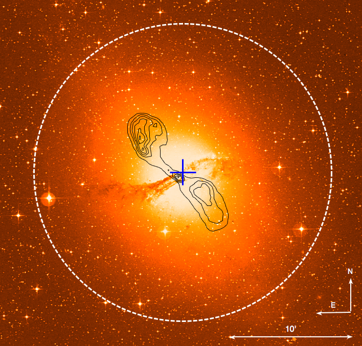
Figure 12: Optical image of Cen A (UK 48-inch Schmidt) overlaid with radio contours (black, VLA [83]). H.E.S.S. VHE best fit position with $1\sigma$ statistical errors (blue cross) and VHE extension 95% CL upper limit (white dashed circle) are also shown. From Ref. [84].

EGRET observations of the gamma ray flux for energies $>100\leavevmode\nobreak\ {\rm MeV}$ allow an estimate $L_{\gamma}\sim 10^{41}\ {\rm erg\ s}^{-1}$ for Cen A [90]. This value of $L_{\gamma}$ is consistent with an earlier observation of photons in the TeV-range during a period of elevated $X$-ray activity [91], and is considerably smaller than the estimated bolometric luminosity $L_{\rm bol}\sim 10^{43}{\rm erg\ s}^{-1}$[82]. Recent data from H.E.S.S. have confirmed Cen A as a TeV $\gamma$-ray emitting source [84]. Extrapolating the spectrum measured with EGRET in the GeV regime to VHEs roughly matches the H.E.S.S. spectrum, though the softer end of the error range on the EGRET spectral index is preferred. More recent data from Fermi-LAT established that a large fraction ($>1/2$) of the total $>100\leavevmode\nobreak\ {\rm MeV}$ emission from Cen A emanates from the lobes [92]. For values of $B$ in the 100 $\mu$G range, substantial proton synchrotron cooling is suppressed, allowing production of high energy electrons through photomeson processes. The average energy of synchrotron photons scales as [93]

$$\langle E_{\gamma}^{\rm syn}\rangle\simeq 0.29\ E_{\gamma}^{\rm syn}\,,$$ (27)

and therefore, to account for the observed TeV photons Cen A should harbor a population of ultra-relativistic electrons, with $E_{e}\sim 10^{9}$ GeV. We further note that this would require the presence of protons with energies between one and two orders of magnitude larger, since the electrons are produced as secondaries.

GRBs

GRBs are flashes of high energy radiation that can be brighter, during their brief existence, than any other source in the sky. The bursts present an amazing variety of temporal profiles, spectra, and timescales [94]. Our insights into this phenomenon have been increased dramatically by BATSE observations of over 2000 GRBs, and more recently, by data from SWIFT.

There are several classes of bursts, from single-peaked events, including the fast rise and exponential decaying (FREDs) and their inverse (anti-FREDs), to chaotic structures [95]. There are well separated episodes of emission, as well as bursts with extremely complex profiles. Most of the bursts are time asymmetric, but some are symmetric. Burst timescales range from about 30 ms to several minutes.

The GRB angular distribution appears to be isotropic, suggesting a cosmological origin [96]. Furthermore, the detection of “afterglows” — delayed low energy (radio to $X$-ray) emission — from GRBs has confirmed this via the redshift determination of several GRB host-galaxies [97].

The $\gamma$-ray luminosity implied by cosmological distances is astonishing: $L_{\gamma}\sim 10^{52}$ erg/s. The most popular interpretation of the GRB-phenomenology is that the observable effects are due to the dissipation of the kinetic energy of a relativistic expanding plasma wind, a “fireball” [98]. Although the primal cause of these events is not fully understood, it is generally believed to be associated with the core collapse of massive stars (in the case of long duration GRBs) and stellar collapse induced through accretion or a merger (short duration GRBs) [99].

The very short timescale observed in the light curves indicates an extreme compactness (i.e. distance scale comparable to a light-ms: $r_{0}\sim 10^{7}$ cm) that implies a source which is initially opaque (because of $\gamma\gamma$ pair creation) to $\gamma$-rays

$$\tau_{\gamma\gamma}\sim r_{0}n_{\gamma}^{\rm GRB}\,\sigma_{T}\sim{\sigma_{T}L_{\gamma}\over 4\pi\,r_{0}\,c\,\epsilon_{\gamma}}\sim 10^{15}\,,$$ (28)

where $n_{\gamma}^{\rm GRB}$ is number density of photons at the source and $\epsilon_{\gamma}\simeq 1$ MeV is the characteristic photon energy.

The high optical depth creates the fireball: a thermal plasma of photons, electrons, and positrons. The radiation pressure on the optically thick source drives relativistic expansion (over a time scale $r_{0}/c$), converting internal energy into the kinetic energy of the inflating shell. As the source expands, the optical depth is reduced. If the source expands with a Lorentz factor $\Gamma$, the energy of photons in the source frame is smaller by a factor $\Gamma$ compared to that in the observer frame, and most photons may therefore be below the pair production threshold. Baryonic pollution in this expanding flow can trap the radiation until most of the initial energy has gone into bulk motion with Lorentz factors of $\Gamma\sim 10^{2}-10^{3}$ [100]. The kinetic energy can be partially converted into heat when the shell collides with the interstellar medium or when shocks within the expanding source collide with one another. The randomized energy can then be radiated by synchrotron radiation and inverse Compton scattering yielding non-thermal bursts with timescales of seconds at large radii, $r>10^{12}\leavevmode\nobreak\ {\rm cm}$, beyond the Thompson sphere. Charged particles may be efficiently accelerated to ultrahigh energies in the fireball’s internal shocks, hence GRBs are often considered as potential sources of UHECRs [101].

Coburn and Boggs [102] reported the detection of polarization, a particular orientation of the electric-field vector, in the $\gamma$-rays observed from a burst. The radiation released through synchrotron emission is highly polarized, unlike in other previously suggested mechanisms such as thermal emission or energy loss by relativistic electrons in intense radiation fields. Thus, polarization in the $\gamma$-rays from a burst provides direct evidence in support of synchrotron emission as the mechanism of $\gamma$-ray production (see also [103]).

Following Hillas criterion, the Larmor radius $r_{L}$ should be smaller than the largest scale $l_{\rm GRB}$ over which the magnetic field fluctuates, since otherwise Fermi acceleration will not be efficient. One may estimate $l_{\rm GRB}$ as follows. The comoving time, i.e. the time measured in the fireball rest frame, is $t=r/\Gamma c$. Hence, the plasma wind properties fluctuate over comoving scale length up to $l_{\rm GRB}\sim r/\Gamma$, because regions separated by a comoving distance larger than $r/\Gamma$ are causally disconnected. Moreover, the internal energy is decreasing because of the expansion and thus it is available for proton acceleration (as well as for $\gamma$-ray production) only over a comoving time $t$. The typical acceleration time scale is then [101]

$$\tau_{\rm acc}^{\rm GRB}\sim\frac{r_{L}}{c}\,.$$ (29)

Equation (29) sets a constraint on the required comoving magnetic field strength, and the Larmor radius $r_{L}=E^{\prime}/eB=E/\Gamma eB$, where $E^{\prime}=E/\Gamma$ is the proton energy measured in the fireball frame. This constraint sets a lower limit to the magnetic field carried by the wind, which may be expressed as

$$\frac{\zeta_{B}}{\zeta_{e}}>0.02\frac{\Gamma_{2.5}^{2}E_{20}^{2}}{L_{52}},$$ (30)

where $\Gamma=10^{2.5}\Gamma_{2.5}$, $L_{\gamma}=10^{52}L_{52}\leavevmode\nobreak\ {\rm erg}\,{\rm\ s}^{-1}.$ Here, $\zeta_{B}$ is the fraction of the wind energy density which is carried by the magnetic field, $4\pi r^{2}\Gamma^{2}(B^{2}/8\pi)=\zeta_{B}L,$ and $\zeta_{e}$ is the fraction of wind energy carried by shock accelerated electrons. Note that because the electron energy is lost radiatively, $L_{\gamma}\approx\zeta_{e}L$.

The dominant energy loss process in this case is synchrotron cooling. Therefore, the condition that the synchrotron loss time of Eq. (21) be smaller than the acceleration time sets the upper limit on the magnetic field strength [101]

$$B<3\times 10^{5}\ \Gamma_{2.5}^{2}\ E_{20}^{-2}\leavevmode\nobreak\ {\rm G}.$$ (31)

Since the equipartition field is inversely proportional to the radius $r$, this condition may be satisfied simultaneously with (30) provided that the dissipation radius is large enough, i.e.

$$r>10^{12}\ \Gamma_{2.5}^{-2}\ E_{20}^{3}\leavevmode\nobreak\ {\rm cm}.$$ (32)

The high energy protons also lose energy in interaction with the wind photons (mainly through pion production). It can be shown, however, that this energy loss is less important than the synchrotron energy loss [101].

In summary, a dissipative ultra-relativistic wind, with luminosity and variability time implied by GRB observations, satisfies the constraints necessary to accelerate protons to energy $\gtrsim 10^{11}$ GeV, provided that $\Gamma>100$, and the magnetic field is close to equipartition with electrons.

0.2.3 Energy losses of baryonic cosmic rays on the pervasive radiation fields

Opacity of the CMB to UHECR protons

Ultrahigh energy protons degrade their energy through Bethe-Heitler (BH) pair production $(p\gamma\rightarrow pe^{+}e^{-}$) and photopion production ($p\gamma\rightarrow\pi N$), each successively dominating as the proton energy increases. The fractional energy loss due to interactions with the cosmic background radiation at a redshift $z=0$ is determined by the integral of the nucleon energy loss per collision multiplied by the probability per unit time for a nucleon collision in an isotropic gas of photons [104]. This integral can be explicitly written as follows,

$$-\frac{1}{E}\frac{dE}{dt}=\frac{c}{2\Gamma^{2}}\,\sum_{j}\,\int_{0}^{\omega_{m}}d\omega_{r}\,\,y_{j}\,\,\sigma_{j}(\omega_{r})\,\,\omega_{r}\,\int_{\omega_{r}/2\Gamma}^{\omega_{m}}d\omega\,\frac{n_{\gamma}(\omega)}{\omega^{2}}\,,$$ (33)

where $\omega_{r}$ is the photon energy in the rest frame of the nucleon, and $y_{j}$ is the inelasticity, i.e. the average fraction of the energy lost by the photon to the nucleon in the laboratory frame for the $j$th reaction channel. (Here the laboratory frame is the one in which the CMB is at a temperature $\approx 2.7$ K.) The sum is carried out over all channels, $n_{\gamma}(\omega)d\omega$ stands for the number density of photons with energy between $\omega$ and $d\omega$, $\sigma_{j}(\omega_{r})$ is the total cross section of the $j$th interaction channel, $\Gamma$ is the usual Lorentz factor of the nucleon, and $\omega_{m}$ is the maximum energy of the photon in the photon gas.

Pair production and photopion production processes are only of importance for interactions with the 2.7 K blackbody background radiation [105]. Collisions with optical and infrared photons give a negligible contribution. Therefore, for interactions with a blackbody field of temperature $T$, the photon density is that of a Planck spectrum, so the fractional energy loss is given by

$$-\frac{1}{E}\frac{dE}{dt}=-\frac{ckT}{2\pi^{2}\Gamma^{2}(c\hbar)^{3}}\sum_{j}\int_{\omega_{0_{j}}}^{\infty}d\omega_{r}\,\sigma_{j}(\omega_{r})\,y_{j}\,\omega_{r}\,\ln(1-e^{-\omega_{r}/2\Gamma kT})\,,$$ (34)

where $\omega_{0_{j}}$ is the threshold energy for the $j$th reaction in the rest frame of the nucleon.

At energies $E\ll m_{e}\,m_{p}/kT=2.1\times 10^{9}$ GeV (i.e., $\omega_{r}/m_{e}-2\ll 1$), when the reaction takes place on the photons from the high energy tail of the Planck distribution, the fraction of energy lost in one collision and the cross section can be approximated by the threshold values

$$y_{{}_{\rm BH}}=2\,\frac{m_{e}}{m_{p}}\,,$$ (35)

and

$$\sigma_{{}_{\rm BH}}(\omega_{r})=\frac{\pi}{12}\,\alpha\,\,r_{0}^{2}\,\,\left(\frac{\omega_{r}}{m_{e}}-2\right)^{3}\,,$$ (36)

where $\alpha$ is the fine structure constant and $r_{0}$ is the classical radius of the electron [105]. The fractional energy loss due to pair production for $E\lesssim 10^{9}$ GeV is then,

$$-\frac{1}{E}\,\left(\frac{dE}{dt}\right)_{\rm BH}=\frac{16c}{\pi}\,\frac{m_{e}}{m_{p}}\,\alpha\,r_{0}^{2}\,\left(\frac{kT}{hc}\right)^{3}\,\left(\frac{\Gamma kT}{m_{e}}\right)^{2}\,\exp\left(-\frac{m_{e}}{\Gamma kT}\right).$$ (37)

At higher energies ($E>10^{10}$ GeV) the characteristic time for the energy loss due to pair production is $t\approx 5\times 10^{9}$ yr [106]. In this energy regime, the photopion reactions $p\gamma\rightarrow p\pi^{0}$ and $p\gamma\rightarrow\pi^{+}n$ on the tail of the Planck distribution give the main contribution to proton energy loss. The cross sections of these reactions are well known and the kinematics is simple.

Photopion production turns on at a photon energy in the proton rest frame of 145 MeV with a strongly increasing cross section at the $\Delta(1232)$ resonance, which decays into the one pion channels $\pi^{+}n$ and $\pi^{0}p$. With increasing energy, heavier baryon resonances occur and the proton might reappear only after successive decays of resonances. The most important channel of this kind is $p\gamma\rightarrow\Delta^{++}\pi^{-}$ with intermediate $\Delta^{++}$ states leading finally to $\Delta^{++}\rightarrow p\pi^{+}$. $\Delta^{++}$ examples in this category are the $\Delta(1620)$ and $\Delta(1700)$ resonances. The cross section in this region can be described by either a sum or a product of Breit-Wigner distributions over the main resonances produced in $N\gamma$ collisions considering $\pi N$, $\pi\pi N$ and $K\Lambda$ ($\Lambda\rightarrow N\pi$) final states [107]. At high energies, $3.0\,{\rm GeV}<\omega_{r}<183\,{\rm GeV}$, the CERN-HERA and COMPAS Groups have made a fit to the $p\gamma$ cross section [108]. The parameterization is

$$\sigma_{\pi}(\omega_{r})=A+B\,\,\ln^{2}\left(\frac{\omega_{r}}{{\rm GeV}}\right)+C\,\,\ln\left(\frac{\omega_{r}}{{\rm GeV}}\right)\,\,{\rm mb}\,,$$ (38)

where $A=0.147\pm 0.001$, $B=0.0022\pm 0.0001$, and $C=-0.0170\pm 0.0007$. In this energy range, the $\sigma_{{\rm total}}(n\gamma)$ is to a good approximation identical to $\sigma_{{\rm total}}(p\gamma)$.

We turn now to the kinematics of photon-nucleon interactions. The inelasticity $y_{\pi}$ depends not only on the outgoing particles but also on the kinematics of the final state. Nevertheless, averaging over final state kinematics leads to a good approximation of $y_{\pi}$. The c.m. system quantities (denoted by $*$) are determined from the relativistic invariance of the square of the total 4-momentum $p_{\mu}p^{\mu}$ of the photon-proton system. This invariance leads to the relation

$$s=(\omega^{*}+E^{*})^{2}=m_{p}^{2}+2m_{p}\omega_{r}.$$ (39)

The c.m. system energies of the particles are uniquely determined by conservation of energy and momentum. For reactions mediated by resonances one can assume a decay, which in the c.m. frame is symmetric in the forward and backward directions with respect to the collision axis (given by the incoming particles). For instance, we consider single pion production via the reaction $p\gamma\rightarrow\Delta\rightarrow p\pi.$ Here,

$$E_{\Delta}^{*}=\frac{(s+m_{\Delta}^{2}-m_{\pi}^{2})}{2\,\sqrt{s}}\,.$$ (40)

Thus, the mean energy of the outgoing proton is

$$\langle E_{p}^{*{\rm final}}\rangle=\frac{(s+m_{\Delta}^{2}-m_{\pi}^{2})}{2\,\sqrt{s}\,m_{\Delta}}\frac{(m^{2}_{\Delta}+m_{p}^{2}-m_{\pi}^{2})}{2\,m_{\Delta}},$$ (41)

or in the lab frame

$$\langle E_{p}^{\rm final}\rangle=\frac{E}{s}\frac{(s-m_{\pi}^{2}+m_{\Delta}^{2})}{2\,m_{\Delta}}\frac{(m_{\Delta}^{2}-m_{\pi}^{2}+m_{p}^{2})}{2\,m_{\Delta}}.$$ (42)

The mean inelasticity $y_{\pi}=1-(\langle E^{\rm final}\rangle/E)$ of a reaction that provides a proton after $n$ resonance decays can be obtained by straightforward generalization of Eq. (42), and is given by

$$y_{\pi}(m_{R_{0}})=1-\frac{1}{2^{n}}\prod_{i=1}^{n}\left(1+\frac{m_{R_{{}_{i}}}^{2}-m_{M}^{2}}{m_{R_{{}_{i-1}}}^{2}}\right)\,,$$ (43)

where $m_{R_{{}_{i}}}$ denotes the mass of the $i^{\rm th}$ resonant system of the decay chain, $m_{M}$ the mass of the associated meson, $m_{R_{{}_{0}}}=\sqrt{s}$ is the total energy of the reaction in the c.m., and $m_{R_{{}_{n}}}$ the mass of the nucleon. For multi-pion production the case is much more complicated because of the non-trivial final state kinematics. However, it is well established experimentally [109] that, at very high energies ($\sqrt{s}\gtrsim 3$ GeV), the incoming particles lose only one-half their energy via pion photoproduction independently of the number of pions produced, $y_{\pi}\sim 1/2$. This is the “leading particle effect”.

For $\sqrt{s}<2$ GeV, the best maximum likelihood fit to Eq. (34) with the exponential behavior

$$-\frac{1}{E}\,\left(\frac{dE}{dt}\right)_{\pi}=A\,{\rm exp}[-B/E]\,,$$ (44)

derived from the values of cross section and fractional energy loss at threshold, gives [110]

$$A=(3.66\pm 0.08)\times 10^{-8}\,{\rm yr}^{-1},\,\,\,\,\,B=(2.87\pm 0.03)\times 10^{11}\,{\rm GeV}\,.$$ (45)

The fractional energy loss due to production of multipion final states at higher c.m. energies ($\sqrt{s}\gtrsim 3$ GeV) is roughly a constant,

$$-\frac{1}{E}\,\left(\frac{dE}{dt}\right)_{\pi}=C=(2.42\pm 0.03)\times 10^{-8}\,\,{\rm yr}^{-1}\,.$$ (46)

From the values determined for the fractional energy loss, it is straightforward to compute the energy degradation of UHECRs in terms of their flight time. This is given by,

$$A\,t\,-\,{\rm Ei}\,(B/E)+\,{\rm Ei}\,(B/E_{0})=0\,,\,\,\,\,\,\,{\rm for}\,\,10^{10}\,{\rm GeV}\lesssim E\lesssim 10^{12}\,{\rm GeV}\,,$$ (47)

and

$$E(t)=E_{0}\exp[-\,C\ t\,]\,,\,\,\,\,\,\,{\rm for}\,\,E\gtrsim 10^{12}\,{\rm GeV}\,,$$ (48)

where Ei is the exponential integral [111]. Figure 13 shows the proton energy degradation as a function of the mean flight distance. Notice that, independent of the initial energy of the nucleon, the mean energy values approach $10^{11}$ GeV after a distance of $\approx 100\leavevmode\nobreak\ {\rm Mpc}$.

Figure 13: Energy attenuation length of protons in the intergalactic medium. Note that after a distance of $\sim 100$ Mpc, or propagation time $\sim 3\times 10^{8}$ yr, the mean energy is essentially independent of the initial energy of the protons, with a critical energy around $10^{11}$ GeV. From Ref. [110].

Photonuclear interactions

The relevant mechanisms for the energy loss that extremely high energy nuclei suffer during their trip to Earth are: Compton interactions, pair production in the field of the nucleus, photodisintegration, and hadron photoproduction. The Compton interactions have no threshold energy. In the nucleus rest-frame, pair production has a threshold at $\sim 1$ MeV, photodisintegration is particularly important at the peak of the GDR (15 to 25 MeV), and photomeson production has a threshold energy of $\sim 145$ MeV.

Compton interactions result in only a negligibly small energy loss for the nucleus given by [112]

$$-\frac{dE}{dt}=\frac{Z^{4}}{A^{2}}\rho_{\gamma}\left(\frac{E}{Am_{p}c^{2}}\right)^{2}\,\,\,{\rm eV\,s^{-1}}\,$$ (49)

where $\rho_{\gamma}$ is the energy density of the ambient photon field in eV cm^-3, $E$ is the total energy of the nucleus in eV, and $Z$ and $A$ are the atomic number and weight of the nucleus. The energy loss rate due to photopair production is $Z^{2}/A$ times higher than for a proton of the same Lorentz factor [113], whereas the energy loss rate due to photomeson production remains roughly the same. The latter is true because the cross section for photomeson production by nuclei is proportional to the mass number $A$ [114], while the inelasticity is proportional to $1/A$. However, it is photodisintegration rather than photopair and photomeson production that determines the energetics of UHECR nuclei. During this process some fragments of the nuclei are released, mostly single neutrons and protons. Experimental data of photonuclear interactions are consistent with a two-step process: photoabsorption by the nucleus to form a compound state, followed by a statistical decay process involving the emission of one or more nucleons.

Following the conventions of Eq. (33), the disintegration rate with production of $i$ nucleons is given by [115]

$$R_{Ai}=\frac{1}{2\Gamma^{2}}\int_{0}^{\infty}d\omega\,\frac{n_{\gamma}(\omega)}{\omega^{2}}\,\int_{0}^{2\Gamma\omega}d\omega_{r}\,\omega_{r}\sigma_{Ai}(\omega_{r})$$ (50)

with $\sigma_{Ai}$ the cross section for the interaction.

The photoabsorption cross section roughly obeys the Thomas-Reiche-Kuhn (TRK) dipole sum rule

$$\Sigma_{d}\equiv\int_{0}^{\infty}\sigma(\omega_{r})d\omega_{r}=59.8\,\frac{N\,Z}{A}\,\,{\rm MeV\,mb}\,,$$ (51)

where $N=A-Z$ is the number of neutrons. (Indeed, this integral is experimentally $\sim 20-30\%$ larger, e.g. for ⁵⁶Fe, $1,020$ mb-MeV for the left hand side, 22% larger than the right hand side [116].) These cross sections contain essentially two regimes. At $\omega_{r}<30$ MeV there is the domain of the GDR where disintegration proceeds mainly by the emission of one or two nucleons. A Gaussian distribution in this energy range is found to adequately fit the cross section data [112]. At higher energies, the cross section is dominated by multinucleon emission and is approximately flat up to $\omega_{r}\sim 150$ MeV. Specifically,

$$\sigma_{Ai}=\frac{\xi_{Ai}\Sigma_{d}\,\Theta(w_{r}-2)\,\Theta(30-\omega_{r})\,e^{-2(\omega_{r}-\epsilon_{0i})^{2}/\Delta_{i}^{2}}}{W\Delta_{i}}+\frac{f_{i}\Sigma_{d}\,\Theta(\omega_{r}-30)}{120}\,,$$ (52)

for $i$=1, 2, and

$$\sigma_{Ai}=\frac{f_{i}\Sigma_{d}\,\Theta(\omega_{r}-30)}{120}\,,$$ (53)

for $i>2$ [112]. Here, $W$ is a normalization factor given by

$$W=\left(\frac{\pi}{8}\right)^{2}\left[\Phi(\sqrt{2}(30-\epsilon_{0i})/\Delta_{i})+\Phi(\sqrt{2}(\epsilon_{0i}-2)/\Delta_{i})\right],$$

$\Phi(x)$ is the error function, and $\Theta(x)$ the Heaviside step function. The dependence of the width $\Delta_{i}$, the peak energy $\epsilon_{0i}$, the branching ratio $f_{i}$, and the dimensionless integrated cross section $\xi_{i}$ are given in Ref. [112] for isotopes up to ⁵⁶Fe.

The photon background relevant for nucleus disintegration consists essentially of photons of the 2.7 K CMB. The background of optical radiation turns out to be of (almost) no relevance for UHECR propagation. The cosmic infrared background (CIB) radiation [117]

$$\frac{dn_{\gamma}(\omega)}{d\omega}=1.1\times 10^{-4}\,\left(\frac{\omega}{{\rm eV}}\right)^{-2.5}\,\,{\rm cm}^{-3}\,{\rm eV}^{-1}\,,$$ (54)

only leads to sizeable effects far below $10^{11}$ GeV and for time-scales ${\cal O}$ ($10^{17}$ s) [118].

By substituting Eqs. (52) and (53) into Eq. (50) the photodisintegration rates on the CMB can be expressed as integrals of two basic forms. The first one is

$$I_{1}=\frac{{\cal A}}{2\Gamma^{2}\pi^{2}\hbar^{3}c^{2}}\left[\int_{1/\Gamma}^{15/\Gamma}d\omega(e^{\omega/kT}-1)^{-1}{\cal J}+\int_{15/\Gamma}^{\infty}d\omega(e^{\omega/kT}-1)^{-1}{\cal J^{\prime}}\right]\,,$$ (55)

where the functions ${\cal J}$ and ${\cal J^{\prime}}$ are given by the expressions,

$${\cal J} = \sqrt{\frac{\pi}{8}}\epsilon_{0i}\Delta_{i}\left[\Phi(\sqrt{2}(2\Gamma\omega-\epsilon_{0i})/\Delta_{i})+\Phi(\sqrt{2}(\epsilon_{0i}-2)/\Delta_{i})\right]$$

$$+ \left(\frac{\Delta_{i}}{2}\right)^{2}\left\{e^{-2((\epsilon_{0i}-2)/\Delta_{i})^{2}}-e^{-2((2\Gamma\omega-\epsilon_{0i})/\Delta_{i})^{2}}\right\}\,,$$

and

$${\cal J^{\prime}} = \sqrt{\frac{\pi}{8}}\epsilon_{0i}\Delta_{i}\left[\Phi(\sqrt{2}(30-\epsilon_{0i})/\Delta_{i})+\Phi(\sqrt{2}(\epsilon_{0i}-2)/\Delta_{i})\right]$$

$$+ \left(\frac{\Delta_{i}}{2}\right)^{2}\left\{e^{-2((\epsilon_{0i}-2)/\Delta_{i})^{2}}-e^{-2((30-\epsilon_{0i})/\Delta_{i})^{2}}\right\}.$$

The second basic integral is of the form

$$I_{2}=(\pi^{2}\hbar^{3}c^{2})^{-1}\sigma_{Ai}\left[\int_{15/\Gamma}^{\infty}\frac{\omega^{2}d\omega}{e^{\omega/kT}-1}-\left(\frac{15}{\Gamma}\right)^{2}\int_{15/\Gamma}^{\infty}\frac{d\omega}{e^{\omega/kT}-1}\right].$$ (58)

With this in mind, Eq. (50) can be re-written as [119]

$$R_{Ai} = \frac{1}{\pi^{2}\hbar^{3}c^{2}\Gamma^{2}}\left\{\frac{{\cal A}}{2}\left(\frac{\pi}{8}\right)^{1/2}\epsilon_{0i}\Delta_{i}\left[e^{-2\epsilon_{0i}^{2}/\Delta_{i}^{2}}{\cal S}_{1}+{\cal S}_{2}\right]-\frac{{\cal A}}{2}\,{\cal J^{\prime}}kT\ln(1-e^{-15/\Gamma kT})\right.$$ (59)

$$-\frac{{\cal A}}{8}\,e^{-2\epsilon_{0i}^{2}/\Delta_{i}^{2}}\left(\frac{\pi}{32}\right)^{1/2}\frac{\Delta_{i}^{3}}{\Gamma}{\cal S}_{3}+\frac{{\cal A}}{2}\,{\cal K}kT\left[\ln(1-e^{-15/\Gamma kT})-\ln(1-e^{-1/\Gamma kT})\right]$$

$$+\left.\frac{f_{i}\Sigma_{d}}{120}\left[\Gamma^{2}{\cal S}_{4}+15^{2}kT\ln(1-e^{-15/\Gamma kT})\right]\right\}\,,$$

with ${\cal A}$, ${\cal S}_{i}$, and ${\cal K}$ as given in Table 2. Summing over all the possible channels for a given number of nucleons, one obtains the effective nucleon loss rate $R_{A}=\sum_{i}iR_{Ai}$. The effective nucleon loss rate for light elements, as well as for those in the carbon, silicon and iron groups can be scaled as [112]

$$\left.\frac{dA}{dt}\right|_{A}\sim\left.\frac{dA}{dt}\right|_{{}^{56}{\rm Fe}}\left(\frac{A}{56}\right)=R_{56}\left(\frac{A}{56}\right)\,.$$ (60)

with the photodisintegration rate (59) parametrized by [120]

$$R_{56}(\Gamma)=3.25\times 10^{-6}\,\Gamma^{-0.643}\exp(-2.15\times 10^{10}/\Gamma)\,\,{\rm s}^{-1}$$ (61)

for $\Gamma\,\in\,[1.0\times 10^{9},36.8\times 10^{9}]$, and

$$R_{56}(\Gamma)=1.59\times 10^{-12}\,\Gamma^{-0.0698}\,\,{\rm s}^{-1}$$ (62)

for $\Gamma\,\in\,[3.68\times 10^{10},10.0\times 10^{10}]$.

EXERCISE 2.1 Approximating the cross section in Eq. (52) by the single pole of the Narrow-Width Approximation [121]

$$\sigma_{A}(\omega^{\prime})=\pi\sigma_{0}\,\frac{\Gamma_{\rm\!GDR}}{2}\,\delta(\omega^{\prime}-\omega_{0})\,,$$ (63)

show that for interactions with the CMB photons

$$R_{A}\approx\frac{\sigma_{0}\,\omega_{0}^{\prime}\,\Gamma_{\rm\!GDR}\ T}{4\Gamma^{2}\pi}\,\left|\ln\left(1-e^{-\omega^{\prime}_{0}/2\Gamma T}\right)\right|\,,$$ (64)

where $\sigma_{0}/A=1.45\times 10^{-27}{\rm cm}^{2}$, $\Gamma_{\rm\!GDR}=8\leavevmode\nobreak\ {\rm MeV}$, and $\epsilon^{\prime}_{0}=42.65A^{-0.21}\,(0.925A^{2.433})\leavevmode\nobreak\ {\rm MeV},$ for $A>4$ ($A\leq 4$) [122]. Verify that for ⁵⁶Fe this solution agrees to within 20% with the parametrization given in Eq. (61).

Table 2: Series and functions of Eq. (59).

${\cal A}$	$W^{-1}\xi_{Ai}\Sigma_{d}\Delta_{i}^{-1}$
${\cal S}_{1}$	$\sum_{{}_{j=1}}^{{}^{\infty}}\,\,kTj^{{}^{-1}}\,\exp[{\cal B}^{{}^{2}}]\,\{\Phi({\cal B}+15\sqrt{8}/\Delta_{i})-\Phi({\cal B}+\sqrt{8}/\Delta_{i})\}$
${\cal S}_{2}$	$\sum_{{}_{j=1}}^{{}^{\infty}}\,\,kTj^{{}^{-1}}\,\exp\{-j/\Gamma kT\}[\Phi(\sqrt{2}(2-\epsilon_{0i})/\Delta_{i})-\Phi(\sqrt{2}(30-\epsilon_{0i})/\Delta_{i})]$
${\cal S}_{3}$	$\sum_{{}_{j=1}}^{{}^{\infty}}\,\,\exp[{\cal B}^{{}^{2}}]\,\{\Phi({\cal B}+15\sqrt{8}/\Delta_{i})-\Phi({\cal B}+\sqrt{8}/\Delta_{i})\}$
${\cal S}_{4}$	$\sum_{{}_{j=1}}^{{}^{\infty}}\exp\{-15j/\Gamma kT\}[(kT/j)(15/\Gamma)^{2}+(kT/j)^{2}(15/\Gamma)+(kT/j)^{3}\,]$
${\cal B}$	$j\Delta_{i}/\Gamma kT\sqrt{32}-2\epsilon_{0i}/\sqrt{2}\Delta_{i}$
${\cal K}$	$\sqrt{\frac{\pi}{8}}\,\epsilon_{0i}\,\Delta_{i}\,\;\Phi(\sqrt{2}\,(\epsilon_{0i}-2)/\Delta_{i})+(\Delta_{i}/2)^{2}\exp\{-2(\epsilon_{0i}-2)^{2}/\Delta_{i}^{2}\}$

For photodisintegration, the averaged fractional energy loss results equal the fractional loss in mass number of the nucleus, because the nucleon emission is isotropic in the rest frame of the nucleus. During the photodisintegration process the Lorentz factor of the nucleus is conserved, unlike the cases of pair production and photomeson production processes which involve the creation of new particles that carry off energy. The total fractional energy loss is then

$$-\frac{1}{E}\frac{dE}{dt}=\frac{1}{\Gamma}\frac{d\Gamma}{dt}+\frac{R}{A}\,.$$ (65)

For $\omega_{r}\lesssim 145$ MeV the reduction in $\Gamma$ comes from the nuclear energy loss due to pair production. The $\gamma$-ray momentum absorbed by the nucleus during the formation of the excited compound nuclear state that precedes nucleon emission is ${\cal O}(10^{-2})$ times the energy loss by nucleon emission [123]. For $\Gamma>10^{10}$ the energy loss due to photopair production is negligible, and thus

$$E(t) \sim 938\,\,A(t)\,\,\Gamma\,\,\,{\rm MeV}$$ (66)

$$\sim E_{0}\,\exp\left[\frac{-R_{56}(\Gamma)\,t}{56}\right]\,.$$

Figure 14: The energy of the surviving fragment ($\Gamma_{0}=4\times 10^{9}$, $\Gamma_{0}=2\times 10^{10}$) vs. propagation time obtained using Eq. (66) is indicated with a solid line. Also included is the energy attenuation length obtained from Monte Carlo simulations with (dashed) and without (dotted-dashed) pair creation production, for comparison. The region between the two dotted lines includes 95% of the simulations. This gives a clear idea of the range of values which can result from fluctuations from the average behaviour. It is important to keep in mind that a light propagation distance of $1.03\times 10^{14}$ s corresponds to 1 Mpc. From Ref. [124].

Figure 14 shows the energy of the heaviest surviving nuclear fragment as a function of the propagation time, for initial iron nuclei. The solid curves are obtained using Eq. (66), whereas the dashed and dotted-dashed curves are obtained by means of Monte Carlo simulations [118]. One can see that nuclei with Lorentz factors above $10^{10}$ cannot survive for more than 10 Mpc. For these distances, the approximation given in Eq. (66) always lies in the region which includes 95% of the Monte Carlo simulations. When the nucleus is emitted with a Lorentz factor $\Gamma_{0}<5\times 10^{9}$, pair production losses start to be relevant, significantly reducing the value of $\Gamma$ as the nucleus propagates distances of ${\cal O}(100\leavevmode\nobreak\ {\rm Mpc})$. The effect has a maximum for $\Gamma_{0}\approx 4\times 10^{9}$ but becomes small again for $\Gamma_{0}\leq 10^{9}$, for which appreciable effects only appear for cosmological distances ($>1000$ Mpc), see for instance [118].

Note that Eq. (66) imposes a strong constraint on the location of nucleus-sources: less than 1% of iron nuclei (or any surviving fragment of their spallations) can survive more than $3\times 10^{14}$ s with an energy $>10^{11.5}$ GeV. For straight line propagation, this represents a maximum distance of $\sim 3$ Mpc.

0.2.4 Diffuse propagation of protons in a magnetized Local Supercluster

In addition to the interactions with the radiation fields permeating the universe, baryonic CRs suffer deflection and delay in magnetic fields, effects which can camouflage their origins. For example, the regular component of the Galactic magnetic field can distort the angular images of CR sources: the flux may appear dispersed around the source or globally translated in the sky with rather small dispersion, viz. the deflection for CRs of charge $Ze$ and energy $E$ should not exceed $\sim 10^{\circ}\,Z\,(4\times 10^{10}\leavevmode\nobreak\ {\rm GeV}/E)$ [125].

One interesting possibility to explain the observed near-isotropy of arrival directions is to envisage a large scale extragalactic magnetic field that can provide sufficient bending to the CR trajectories. Surprisingly little is actually known about the extragalactic magnetic field strength. There are some measurements of diffuse radio emission from the bridge area between the Coma and Abell superclusters [126], which under assumptions of equipartition allows an estimate of ${\cal O}(0.2-0.6)\,\mu$G for the magnetic field in this region. Fields of ${\cal O}(\mu{\rm G})$ are also indicated in a more extensive study of 16 low redshift clusters [127]. It is assumed that the observed $B$-fields result from the amplification of much weaker seed fields. However, the nature of the initial week seed fields is largely unknown. There are two broad classes of models for seed fields: cosmological models, in which the seed fields are produced in the early universe, and astrophysical models, in which the seed fields are generated by motions of the plasma in (proto)galaxies. Of particular interest here is the second class of models. If most galaxies lived through an active phase in their history, magnetized outflows from their jets and winds would efficiently pollute the extragalactic medium. The resulting $B$-field is expected to be randomly oriented within cells of sizes below the mean separation between galaxies, $\lambda_{B}\lesssim 1\leavevmode\nobreak\ {\rm Mpc}.$

Extremely weak unamplified extragalactic magnetic fields have escaped detection up to now. Measurements of the Faraday rotation in the linearly polarized radio emission from distant quasars [128] and/or distortions of the spectrum and polarization properties in the CMB [129, 130] imply upper limits on the extragalactic magnetic field strength as a function of the reversal scale. It is important to stress that Faraday rotation measurements (RM) sample extragalactic magnetic fields of any origin (out to quasar distances), while the CMB analyses set limits only on primordial magnetic fields. The RM bounds depend significantly on assumptions about the electron density profile as a function of the redshift. When electron densities follow that of the Lyman-$\alpha$ forest, the average magnitude of the magnetic field receives an upper limit of $B\sim 10^{-9}$ G for reversals on the scale of the horizon, and $B\sim 10^{-8}$ G for reversal scales on the order of 1 Mpc [131]. As a statistical average over the sky, an all pervading extragalactic magnetic field is constrained to be [132]

$$B\lesssim 3\times 10^{-7}\,(\Omega_{b}h^{2}/0.02)^{-1}\,(h/0.72)\,(\lambda_{B}/{\rm Mpc})^{1/2}\leavevmode\nobreak\ {\rm G}\,,$$ (67)

where $\Omega_{b}h^{2}\simeq 0.02$ is the baryon density and $h\simeq 0.72$ is the present day normalized Hubble expansion rate. This is a conservative bound because $\Omega_{b}$ has contributions from neutrons and only electrons in ionized gas are relevant to Faraday rotation.

In the spirit of [133, 134], very recently we proposed that neutron emission from Cen A could dominate the observed CR flux above the GZK suppression [135]. Neutrons that are able to decay generate proton diffusion fronts in the intergalactic turbulent magnetic plasma. In our calculations we assume a strongly turbulent magnetic field: $B=50\leavevmode\nobreak\ {\rm nG}$, $\lambda_{B}\sim 1\leavevmode\nobreak\ {\rm Mpc}$, and largest turbulent eddy $\ell\sim 2\pi\lambda_{B}$ [136]. For energies above the GZK supression, $\lambda_{B}\lesssim r_{L}\lesssim\ell$ and so the diffusion coefficient is given by the Bohm formula [75]

$$D(E)=\frac{cr_{L}}{3}=0.1\,\left(\frac{E}{{\rm EeV}}\right)\,\left(\frac{B}{{\rm nG}}\right)^{-1}\leavevmode\nobreak\ {\rm Mpc}^{2}\ {\rm Myr}^{-1}\,.$$ (68)

The evolution of the proton spectrum is driven by the so-called “energy loss-diffusion equation”

$$\frac{\partial n(E,\bm{r},t)}{\partial t}=\frac{\partial[b(E)n(E,\bm{r},t)]}{\partial E}+\bm{\nabla}[D(E,\bm{r},t)\,\bm{\nabla}n(E,\bm{r},t)]+Q(E,t)\,\delta^{3}(x)\,,$$ (69)

where $n(E,\bm{r},0)=N_{0}\ \delta^{3}(x)$. Here, $b(E)\equiv dE/dt$ is the mean rate at which particles lose energy and $Q(E,t)$ is the number of protons per unit energy and per unit time generated by the source. For the situation at hand, $D(E,\bm{r},t)=D(E)$ and hence the second term becomes $D(E)\nabla^{2}n(E,\bm{r},t)$. Idealizing the emission to be uniform with a rate $dN_{0}/dt=N_{\rm tot}/\tau$, we have

$$Q(E,t)=\frac{N_{\rm tot}}{\tau}\,\,[\Theta(t-t_{{\rm on}})-\Theta(t-t_{{\rm off}})],$$ (70)

where $\int{\cal Q}(E,\bm{r}^{\prime},t^{\prime})\,d^{3}x^{\prime}\,dt^{\prime}=N_{\rm tot}$, $\Theta$ is the Heaviside step function, and $t_{{\rm on}}$ ($t_{{\rm off}}$) is the time since the engine turned on (off) its CR production, $t_{{\rm off}}-t_{{\rm on}}=\tau$. For the energy region of interest, the expected time delay of the diffuse protons, $\tau_{\rm delay}\sim d^{2}/D(E),$ is significantly smaller than the characteristic time scale for photopion production derived in Eq. (44).

If the energy loss term is neglected, the solution to Eq. (69) reads,

$$n(E,\bm{r},t)=\int dt^{\prime}\int d^{3}x^{\prime}\,\,G(\bm{r}-\bm{r}^{\prime},t-t^{\prime})\,\,{\cal Q}(E,\bm{r}^{\prime},t^{\prime}),$$ (71)

where

$$G(\bm{r}-\bm{r}^{\prime},t-t^{\prime})=[4\,\pi\,D\,(t-t^{\prime})]^{-3/2}\,\,\Theta(t-t^{\prime})\exp\{-(\bm{r}-\bm{r}^{\prime})^{2}/4D(t-t^{\prime})\}\,,$$ (72)

is the Green function [137]. The density of protons at the present time $t$ of energy $E$ at a distance $\bm{r}$ from Cen A, which is assumed to be continuously emitting at a constant spectral rate $dN_{0}/dE\,dt$ from time $t_{\rm on}$ until the present, is found to be [134]

$$\frac{dn(E,\bm{r},t)}{dE} = \frac{dN_{0}}{dE\,dt}\frac{1}{[4\pi D(E)]^{3/2}}\int_{t_{\rm on}}^{t}dt^{\prime}\,\frac{e^{-r^{2}/4D(t-t^{\prime})}}{(t-t^{\prime})^{3/2}}$$ (73)

$$= \frac{dN_{0}}{dE\,dt}\,\frac{1}{4\pi^{3/2}D(E)r}\int_{v_{1}}^{v_{2}}\frac{dv}{v^{3/2}}\,e^{-1/v}$$

$$= \frac{dN_{0}}{dE\,dt}\frac{1}{4\pi D(E)r}\,\,I(x)\,,$$

where we have used the change of variables

$$u=\frac{r^{2}}{4D(t-t^{\prime})}=\frac{1}{v}\,,$$ (74)

with $x=4DT_{\rm on}/r^{2}$, $T_{\rm on}=t-t_{\rm on},$ and

$$I(x)=\frac{1}{\sqrt{\pi}}\int_{1/x}^{\infty}\frac{du}{\sqrt{u}}\,\,e^{-u}\ \ .$$ (75)

For $T_{\rm on}\rightarrow\infty$, the density approaches its time-independent equilibrium value $n_{\rm eq}$.

As a result of this diffusion the $J\propto E^{-4}$ behavior of the observed CR spectrum reflects a $dN_{0}/dEdt\propto E^{-3}$ injection in the region of the source cutoff. For $S=3000\leavevmode\nobreak\ {\rm km}^{2}$ detector like Auger, the neutron rate is

$$\frac{dN_{n}}{dt}=\frac{S}{4\pi d^{2}}\int_{E_{1}}^{E_{2}}e^{-d/\lambda(E)}\ \frac{dN_{0}}{dEdt}\,dE,$$ (76)

where $\lambda(E)\simeq 9.2\times 10^{-3}\,E_{\rm EeV}\leavevmode\nobreak\ {\rm Mpc}$ is the neutron decay length. For the energy interval between $E_{1}=55\leavevmode\nobreak\ {\rm EeV}$ and $E_{2}=150\leavevmode\nobreak\ {\rm EeV}$, we calculate the normalization factor using the observation of 2 neutrons in 3 yr of the nominal exposure/yr of Auger. We then use this normalization factor to calculate the luminosity of the source in the above energy interval. We find $L_{\rm CR}^{(E_{1},E_{2})}=0.86\times 10^{40}\leavevmode\nobreak\ {\rm erg/s}$ [135]. Next, we assume continuity of the spectrum at $E_{1}$ as it flattens to $E^{-2}.$ Taking the lower bound on the energy to be $E_{0}=10\leavevmode\nobreak\ {\rm EeV}$, we can then fix the luminosity for this interval and find $L_{\rm CR}^{(E_{0},E_{1})}=2.3\times 10^{40}\leavevmode\nobreak\ {\rm erg/s}.$ Adding these, we find the (quasi) bolometric luminosity to be $L_{\rm CR}^{(E_{0},E_{2})}=3.2\times 10^{40}\leavevmode\nobreak\ {\rm erg/s},$ which is about a factor of 3 smaller than the observed luminosity in $E>100\leavevmode\nobreak\ {\rm MeV}$ $\gamma$-rays $L_{\gamma}\approx 10^{41}\leavevmode\nobreak\ {\rm erg/s}$ [90]. To further constrain the parameters of the model, we evaluate the energy-weighted approximately isotropic proton flux at 70 EeV. If the source actively emitted UHECRs for at least 70 Myr, from Eq. (73) we obtain

$$\langle E^{4}\,J(E)\rangle = \frac{E^{4}\,c}{(4\pi)^{2}dD(E)}\,\frac{dN_{0}}{dE\,dt}\,I(x)$$ (77)

$$\approx 1.6\times 10^{57}\leavevmode\nobreak\ {\rm eV}^{3}\,{\rm km}^{-2}\,\rm{yr}^{-1}\,{\rm sr}^{-1}\,,$$

in agreement with observations [29]. If we assume circular pixel sizes with $3^{\circ}$ radii, the neutrons will be collected in a pixel representing a solid angle $\Delta\Omega\simeq 8.6\times 10^{-3}\leavevmode\nobreak\ {\rm sr}$. The event rate of (diffuse) protons coming from the direction of Cen A is found to be

$$\frac{dN_{p}}{dt}=S\ \Delta\Omega\,\int_{E_{1}}^{E_{2}}\langle E^{4}\,J\rangle\ \frac{dE}{E^{4}}=0.08\leavevmode\nobreak\ {\rm events/yr}\,.$$ (78)

All in all, in the next 9 yr of operation we expect about 6 direct neutron events against an almost negligible background. Note that our model also predicts no excess in the direction of M87, in agreement with observations (see Fig. 8).

We turn now to the discussion of anisotropy. The number of particles with velocity $c$ hitting a unit area in a unit time in a uniform gas of density $n(E,\bm{r},t)$ is $n(E,\bm{r},t)\,c$. Due to the gradient in the number density with radial distance from the source, the downward flux at Earth per steradian as a function of the angle $\theta$ to the source is [133]

$$J(\theta,\bm{r},t)=\frac{n(E,\bm{r},t)\,c}{4\pi}(1+\alpha_{d}\cos\theta)\,,$$ (79)

where

$$\alpha_{d}\,\cos\theta=\frac{|\bm{j}(E,\bm{r},t)|}{n(E,\bm{r},t)\,c}\ .$$ (80)

The asymmetry parameter $\alpha_{d}$ can be found by computing the incoming current flux density $\bm{j}=D\bm{\nabla_{r^{\prime}}}n$ as viewed by an observer on Earth, where $\bm{r}=\bm{R}+\bm{r}^{\prime}$. We obtain

$$j^{\prime}_{i}(E,x^{\prime}_{i},t) = D\,\frac{\partial n(E,x^{\prime}_{i},t)}{\partial x^{\prime}_{i}}$$ (81)

$$= D\frac{dN_{0}}{dEdt}\frac{1}{(4\pi D)^{3/2}}\int_{t_{\rm on}}^{t}\frac{dt^{\prime}}{(t-t^{\prime})^{3/2}}e^{-(R^{2}+2\bm{R}\,.\,\bm{r^{\prime}}+r^{\prime 2})/4D(t-t^{\prime})}\,\frac{-(2R_{i}+2x^{\prime}_{i})}{4D(t-t^{\prime})}$$

$$= -\frac{(R_{i}+x^{\prime}_{i})}{2(4\pi D)^{3/2}}\int_{t_{\rm on}}^{t}\frac{dt^{\prime}}{(t-t^{\prime})^{5/2}}\,e^{-r^{2}/[4D(t-t^{\prime})]}\ .$$

Near $x^{\prime}_{i}=0$, using the change of variables in Eq. (74), we obtain

$$j^{\prime}_{i}(E,x^{\prime}_{i},t) = \frac{R_{i}}{2}\frac{dN_{0}}{dEdt}\frac{1}{(4\pi D)^{3/2}}\,\frac{r^{2}}{4D}\left(\frac{4D}{r^{2}}\right)^{5/2}\int_{1/x}^{\infty}du\,u^{1/2}\,e^{-u}$$ (82)

$$= \frac{R_{i}}{2\pi}\,\frac{dN_{0}}{dEdt}\,\frac{1}{r^{3}}\,I^{\prime}(x)\,,$$

where

$$I^{\prime}(x)=\frac{1}{\sqrt{\pi}}\int_{1/x}^{\infty}du\ \sqrt{u}\,\,e^{-u}\,.$$ (83)

Finally, taking $R_{x}=R_{x}=0$ and $R_{z}=r\,\cos\theta$ we obtain [134]

$$\alpha_{d}=\frac{2D(E)}{cr}\ \,\frac{I^{\prime}(x)}{I(x)}\ .$$ (84)

For $T_{\rm on}\rightarrow\infty$, $0\leq\alpha\leq 1$. Taking our fiducial values $E=70\leavevmode\nobreak\ {\rm EeV}$, $B_{\rm nG}=50$, and $T_{\rm on}=70$, we find $\alpha_{d}=0.29$. This is within $\sim 1\sigma$ of the anisotropy amplitude $\alpha_{d}=d_{\perp}/\cos\delta_{0}=0.25\pm 0.18$ obtained from the 69 arrival directions, assuming a dipole function for a source model with a maximum value at Cen A: $(\alpha_{0},\delta_{0})=(201.4^{\circ},-43.0^{\circ})$.

Figure 15: The nominal arrival directions ($\alpha=$ right ascension, $\delta=$ declination) of SUGAR events with energies above $4\times 10^{10}$ GeV [138]. Also shown in solid lines are contour maps indicating the circular areas of the celestial sphere centered at Cen A (indicated by $\star$) with $10^{\circ}$ and $25^{\circ}$ radii. The dashed lines surrounding several of the events indicate the uncertainty of each arrival direction; this was found to be about $3^{\circ}\ {\rm sec}\leavevmode\nobreak\ \theta,$ where $\theta$ is the shower zenith angle. From Ref. [81].

One caveat is that we assumed that neutrons completely dominate the ultrahigh energy Cen A emission spectrum; that is

$$\frac{dN_{0}}{dE\,dt}=(N_{0}^{n}+N_{0}^{p})E^{-3}\,,{\quad}{\rm with}{\quad}N_{0}^{p}/N_{0}^{n}\ll 1\,.$$ (85)

This reduces the number of free parameters in the model. The actual proton-to-neuton fraction depends on the properties of the source, dominantly by the ratio of photon-to-magnetic energy density. The relation (85) results from $a\sim 0.4,$ which implies that photopion production – and not proton leakege from the accelerator region – determines the shape of the cutoff in the spectrum at the source.

EXERCISE 2.2 The assymetry parameter given in Eq. (84) accurately describes the diffuse propagation of CRs if $N_{0}^{n}/N_{0}^{p}\ll 1$. Show that asymmetry parameter from the neutron decay shell is given by

$$\alpha_{d}=\frac{2D(E)}{cr}\,\frac{I^{\prime\prime}(x)}{I(x)}\ \ \ ,$$ (86)

where

$$I^{\prime\prime}(x)=\frac{1}{4\sqrt{\pi}\kappa}\int_{1/x}^{\infty}\frac{du}{u^{3/2}}\left[\left((1-\kappa)u+\tfrac{1}{2}\right)\ e^{-(1-\kappa)^{2}u}-\left((1+\kappa)u+\tfrac{1}{2}\right)\ e^{-(1+\kappa)^{2}u}\right]$$ (87)

and $\kappa=\lambda(E)/r$. Show that in spite of the complicated nature of Eq.(87), the results for $\alpha_{d}$ are very similar to the ones for the primary diffusion front given above.

An observation demanding of some attention is the distribution of arrival directions of the events collected by the SUGAR experiment, shown in Fig. 15. We take the data at face value keeping in mind that the techniques available at the time the experiment was conducted were not as refined as the techniques currently at our disposal. As one can see in Fig. 15, while the Auger and SUGAR distrbutions are not dissimilar, the statistics are rather limited and do not support a firm conclusion.

As an attentive reader should know by now, the observed excess in the direction of Cen A can also be explained using proton directional signals and diffusion of heavy nuclei in a $B$-field of about 1 nG [139]. However, if this were the case, a larger anisotropy (as yet unobserved) should be present at EeV energies [140]. Regarding the preceeding discussion, one should note that the $3^{\circ}$ window does not have an underlying theoretical motivation. Recall that this angular range resulted from a scan of parameters to maximize signal significance. Cen A covers an eliptical region spanning about $10^{\circ}$ along the major axis; see Fig. 12. Therefore, some care is required to select the region of the sky which is most likely to maximize the signal-to-noise.

In summary, existing data is consistent with the hypothesis that Cen A dominates the CR sky at the high end of the spectrum [133]. Auger is in a gifted position to explore Cen A and would provide in the next 9 yr of operation sufficient statistics to test this hypothesis. The potential detection of neutrons at Auger can subsequently be validated by the larger aperture of the JEM-EUSO mission.

0.2.5 Ultrahigh energy cosmic neutrinos

Waxman-Bahcall bound

It is helpful to envision the CR engines as machines where protons are accelerated and (possibly) permanently confined by the magnetic fields of the acceleration region. The production of neutrons and pions and subsequent decay produces neutrinos, $\gamma$-rays, and CRs. If the neutrino-emitting source also produces high energy CRs, then pion production must be the principal agent for the high energy cutoff on the proton spectrum. Conversely, since the protons must undergo sufficient acceleration, inelastic pion production needs to be small below the cutoff energy; consequently, the plasma must be optically thin. Since the interaction time for protons is greatly increased over that of neutrons due to magnetic confinement, the neutrons escape before interacting, and on decay give rise to the observed CR flux. The foregoing can be summarized as three conditions on the characteristic nucleon interaction time scale $\tau_{\rm int}$; the neutron decay lifetime $\tau_{n}$; the characteristic cycle time of confinement $\tau_{\rm cycle}$; and the total proton confinement time $\tau_{\rm conf}$: $(i)\;\tau_{\rm int}\gg\tau_{\rm cycle}$; $(ii)\;\tau_{n}>\tau_{\rm cycle}$; $(iii)\;\tau_{\rm int}\ll\tau_{\rm conf}$. The first condition ensures that the protons attain sufficient energy. Conditions $(i)$ and $(ii)$ allow the neutrons to escape the source before decaying. Condition $(iii)$ permits sufficient interaction to produce neutrons and neutrinos. These three conditions together define an optically thin source [141]. A desirable property to reproduce the almost structureless energy spectrum is that a single type of source will produce cosmic rays with a smooth spectrum across a wide range of energy.

The cosmic ray flux above the ankle is often summarized as “one $3\times 10^{10}$ GeV particle per kilometer square per year per steradian.” This can be translated into an energy flux [142]

$$E\left\{E{J_{\rm CR}}\right\} = {3\times 10^{10}\,{\rm GeV}\over\rm(10^{10}\,cm^{2})(3\times 10^{7}\,s)\,sr}$$ (88)

$$= 10^{-7}\rm\,GeV\ cm^{-2}\,s^{-1}\,sr^{-1}\,.$$

From this we can derive the energy density $\epsilon_{\rm CR}$ in UHECRs using flux${}={}$velocity${}\times{}$density, or

$$4\pi\int dE\left\{E{J_{\rm CR}}\right\}=c\,\epsilon_{\rm CR}\,.$$ (89)

This leads to

$$\epsilon_{\rm CR}={4\pi\over c}\int_{E_{\rm min}}^{E_{\rm max}}{10^{-7}\over E}dE\,{\rm{GeV\over cm^{2}\,s}}\simeq 10^{-19}\,{\rm{TeV\over cm^{3}}}\,,$$ (90)

taking the extreme energies of the accelerator(s) to be $E_{\rm min}\simeq 10^{10}\leavevmode\nobreak\ {\rm GeV}$ and $E_{\rm max}=10^{12}\leavevmode\nobreak\ {\rm GeV}$. The power required for a population of sources to generate this energy density over the Hubble time (${\cal T}_{H}\approx 10^{10}$ yr) is: $\dot{\epsilon}_{\rm CR}^{[10^{10},10^{12}]}\sim 5\times 10^{44}\leavevmode\nobreak\ {\rm TeV}\,{\rm Mpc}^{-3}\,{\rm yr}^{-1}\simeq 3\times 10^{37}\leavevmode\nobreak\ {\rm erg}\,{\rm Mpc}^{-3}\,{\rm s}^{-1}$. This works out to roughly (i ) $L\approx 3\times 10^{39}$ erg s^-1 per galaxy, (ii ) $L\approx 3\times 10^{42}$ erg s^-1 per cluster of galaxies, (iii ) $L\approx 2\times 10^{44}$ erg s^-1 per active galaxy, or (iv ) $\int L\,dt\approx 10^{52}$ erg per cosmological GRB [142]. The coincidence between these numbers and the observed output in electromagnetic energy of these sources explains why they have emerged as the leading candidates for the CR accelerators.

The energy production rate of protons derived professionally, assuming a cosmological distribution of sources (with injection spectrum typical of shock acceleration $dN_{0}/dE\propto E^{-2}$) is [143]

$$\dot{\epsilon}_{\rm CR}^{[10^{10},10^{12}]}\sim 5\times 10^{44}\leavevmode\nobreak\ {\rm erg}\,{\rm Mpc}^{-3}\,{\rm yr}^{-1}\,.$$ (91)

This is within a factor of our back-of-the-envelope estimate (1 TeV = 1.6 erg). The energy-dependent generation rate of CRs is therefore given by

$$E^{2}\frac{d\dot{n}}{dE} = \frac{\dot{\epsilon}_{\rm CR}^{[10^{10},10^{12}]}}{\ln(10^{12}/10^{10})}$$ (92)

$$\approx 10^{44}\,\rm{erg}\,\rm{Mpc}^{-3}\rm{yr}^{-1}\,\,.$$

The energy density of neutrinos produced through $p\gamma$ interactions of these protons can be directly tied to the injection rate of CRs

$$E^{2}_{\nu}\frac{dn_{\nu}}{dE_{\nu}}\approx\frac{3}{8}\epsilon_{\pi}\,{\cal T}_{H}\,E^{2}\,\frac{d\dot{n}}{dE}\,,$$ (93)

where $\epsilon_{\pi}$ is the fraction of the energy which is injected in protons lost into photopion interactions. The factor of 3/8 comes from the fact that, close to threshold, roughly half the pions produced are neutral, thus not generating neutrinos, and one quarter of the energy of charged pion decays goes to electrons rather than neutrinos. Namely, resonant $p\gamma$ interactions produce twice as many neutral pions as charged pions. Direct pion production via virtual meson exchange contributes only about 20% to the total cross section, but is almost exclusively into $\pi^{+}$. Hence, $p\gamma$ interactions produce roughly equal numbers of $\pi^{+}$ and $\pi^{0}$. The average neutrino energy from the direct pion decay is $\langle E_{\nu_{\mu}}\rangle^{\pi}=(1-r)\,E_{\pi}/2\simeq 0.22\,E_{\pi}$ and that of the muon is $\langle E_{\mu}\rangle^{\pi}=(1+r)\,E_{\pi}/2\simeq 0.78\,E_{\pi}$, where $r$ is the ratio of muon to the pion mass squared. In muon decay, since the $\nu_{\mu}$ has about 1/3 of its parent energy, the average muon neutrino energy is $\langle E_{\nu_{\mu}}\rangle^{\mu}=(1+r)E_{\pi}/6=0.26\,E_{\pi}$.

The “Waxman-Bahcall bound” is defined by the condition $\epsilon_{\pi}=1$

$$E^{2}_{\nu}\ \Phi_{\rm WB}^{\nu_{\rm all}} \approx (3/8)\,\xi_{z}\,\epsilon_{\pi}\,{\cal T}_{H}\,\frac{c}{4\pi}\,E^{2}\,\frac{d\dot{n}}{dE}$$ (94)

$$\approx 2.3\times 10^{-8}\,\epsilon_{\pi}\,\xi_{z}\,\rm{GeV}\,\rm{cm}^{-2}\,\rm{s}^{-1}\,\rm{sr}^{-1},$$

where the parameter $\xi_{z}$ accounts for the effects of source evolution with redshift, and is expected to be $\sim 3$ [144]. For interactions with the ambient gas (i.e. $pp$ rather than $p\gamma$ collisions), the average fraction of the total pion energy carried by charged pions is about $2/3$, compared to $1/2$ in the photopion channel. In this case, the upper bound given in Eq. (94) is enhanced by 33%. Electron antineutrinos can also be produced through neutron $\beta$-decay. This contribution, however, turns out to be negligible (see Appendix .5 for details).

The actual value of the neutrino flux depends on what fraction of the proton energy is converted to charged pions (which then decay to neutrinos), i.e. $\epsilon_{\pi}$ is the ratio of charged pion energy to the emerging nucleon energy at the source. For resonant photoproduction, the inelasticity is kinematically determined by requiring equal boosts for the decay products of the $\Delta^{+}$, giving $\epsilon_{\pi}=E_{\pi^{+}}/E_{n}\approx 0.28$, where $E_{\pi^{+}}$ and $E_{n}$ are the emerging charged pion and neutron energies, respectively. For $pp\rightarrow NN+{\rm pions},$ where $N$ indicates a final state nucleon, the inelasticity is $\approx 0.6$ [145]. This then implies that the energy carried away by charged pions is about equal to the emerging nucleon energy, yielding (with our definition) $\epsilon_{\pi}\approx 1.$

At production, if all muons decay, the neutrino flux consists of equal fractions of $\nu_{e}$, $\nu_{\mu}$ and $\bar{\nu}_{\mu}$. Originally, the Waxman-Bahcall bound was presented for the sum of $\nu_{\mu}$ and $\bar{\nu}_{\mu}$ (neglecting $\nu_{e}$), motivated by the fact that only muon neutrinos are detectable as track events in neutrino telescopes. Since oscillations in the neutrino sector mix the different species, we chose instead to discuss the sum of all neutrino flavors. When the effects of oscillations are accounted for, nearly equal numbers of the three neutrino flavors are expected at Earth [146].

EXERCISE 2.3   The assumption that GRBs are the sources of the observed UHECRs generates a calculable flux of neutrinos produced when the protons interact with the fireball photons [147]. In the observer’s frame, the spectral photon density (${\rm GeV}^{-1}\,{\rm cm}^{-3}$) can be adequately parametrized by a broken power-law spectrum $n_{\gamma}^{\rm GRB}(\epsilon_{\gamma})\propto\epsilon_{\gamma}^{-\beta}$, where $\beta\simeq 1,\ 2$ respectively at energies below and above $\epsilon_{\gamma}^{\rm break}\simeq 1\leavevmode\nobreak\ {\rm MeV}$ [148]. Show that

$$\Phi_{\rm GRB}^{\nu_{\rm all}}(E_{\nu}>E_{\nu}^{\rm break})\sim 10^{-13}\ \left(\frac{E_{\nu}^{\rm break}}{10^{5}\leavevmode\nobreak\ {\rm GeV}}\right)^{-1}\leavevmode\nobreak\ {\rm cm}^{-2}\,{\rm s}^{-1}\,{\rm sr}^{-1}\,,$$ (95)

where $E_{\nu}^{\rm break}\sim 5\times 10^{5}\,\Gamma_{2.5}^{2}(\epsilon_{\gamma}^{\rm break}/{\rm MeV})^{-1}\leavevmode\nobreak\ {\rm GeV}.$ Recall that in our convention $\epsilon_{\gamma}=\Gamma\epsilon^{\prime}_{\gamma}$, where $\epsilon^{\prime}_{\gamma}$ is the photon energy measured in the fireball frame. Convince yourself that the non-observation of extraterrestrial neutrinos from sources other than the Sun and SN1987a puts the GRB model of UHECR acceleration on probation [149].

If the injected cosmic rays include nuclei heavier than protons, then the neutrino flux expected from the cosmic ray sources may be modified. Nuclei undergoing acceleration can produce pions, just as protons do, through interactions with the ambient gas, so the Waxman-Bahcall argument would be unchanged in this case. However, if interactions with radiation fields dominate over interactions with matter, the neutrino flux would be suppressed if the cosmic rays are heavy nuclei. This is because the photodisintegration of nuclei dominates over pion production at all but the very highest energies. Defining $\kappa$ as the fraction of nuclei heavier than protons in the observed cosmic ray spectrum, the resulting neutrino flux is then given by $E^{2}_{\nu}\ \Phi^{\nu_{\rm all}}\approx(1-\kappa)\,\,E^{2}_{\nu}\ \Phi^{\nu_{\rm all}}_{\rm{WB}}\,\,$ [150]. The most up-to-date calculation of $\kappa$ combines a double-fit analysis of the energy and elongation rate measurements to constrain the spectrum and chemical composition of UHECRs at their sources [151]. Injection models with a wide range of chemical composition are found to be consistent with observations. In particular, the data are consistent with a proton dominated spectrum with only a small (1 - 10%) admixture of heavy nuclei.

By duplicating the Waxman-Bahcall calculation for Cen A, we obtain an upper limit on the intensity of neutrinos from the direction of the nearest active galaxy,

$$E_{\nu}^{2}\ \phi_{{}_{\rm Cen\,A}}^{\nu_{\rm all}} = \frac{1}{4\pi d^{2}}\ L_{\rm CR}\ \frac{3}{8}\ \epsilon_{\pi}$$ (96)

$$\approx 5.0\times 10^{-9}\leavevmode\nobreak\ {\rm GeV}\ {\rm cm}^{-2}\ {\rm s}^{-1}\,,$$

with $E_{\nu}\lesssim 10^{9.5}\leavevmode\nobreak\ {\rm GeV}$. For the model introduced in Sec. 0.2.4, we have $\epsilon_{\pi}\sim 0.28$ and therefore a prediction for the all-flavor neutrino flux

$$E_{\nu}^{2}\ \phi_{{}_{\rm Cen\,A}}^{\nu_{\rm all}}\approx 1.5\times 10^{-9}\leavevmode\nobreak\ {\rm GeV}\ {\rm cm}^{-2}\ {\rm s}^{-1}\,,$$ (97)

in agreement with the results of [152]. In addition to neutrinos, one also expects a similar flux of photons at the source, which also carries unperturbed directional information. However, photons at these energies are difficult to dig out from the hughe proton background.

Although there are no other nearby FRI of this magnitude which can potentially be detected as point sources, one can integrate over the estimated FRI population out to the horizon to obtain an upper limit for the diffuse FRI neutrino flux. This quantity is given by [153]

$$E_{\nu}^{2}\ \Phi_{\rm FRI}^{\nu_{\rm all}} = \frac{1}{4\pi}\,{\cal R}_{H}\ n_{{}_{\rm FRI}}\,L_{\rm CR}\ \frac{3}{8}\ \epsilon_{\pi}$$ (98)

$$\approx 1.5\times 10^{-8}\leavevmode\nobreak\ {\rm GeV}\ {\rm cm}^{-2}\ {\rm s}^{-1}\,{\rm sr}^{-1}\,,$$

where ${\cal R}_{H}\simeq 1$ horizon $\simeq 3\leavevmode\nobreak\ {\rm Gpc}$ and $n_{{}_{\rm FRI}}\sim 8\times 10^{4}\leavevmode\nobreak\ {\rm Gpc}^{-3}$ is the number density [154]. Note that this flux is about a factor of 3 smaller than the Waxman-Bahcall upper limit. Hence, the reduction in luminosity of the ensemble of neutrino sources roughly compensates for the presence of distant optically thin sources whose CR components are hidden by extragalactic magnetic fields.

The diffuse neutrino flux has an additional component originating in the energy losses of UHECRs en route to Earth [155]. The accumulation of these neutrinos over cosmological time is known as the cosmogenic neutrino flux. The GZK reaction chain generating cosmogenic neutrinos is well known [156]. The intermediate state of the reaction $p\gamma_{\rm CMB}\to n\pi^{+}/p\pi^{0}$ is dominated by the $\Delta^{+}$ resonance, because the neutron decay length is smaller than the nucleon mean free path on the CMB. Gamma-rays, produced via $\pi^{0}$ decay, subsequently cascade electromagnetically on intergalactic radiation fields through $e^{+}e^{-}$ pair production followed by inverse Compton scattering. The net result is a pile up of $\gamma$-rays at GeV-TeV energies, just below the threshold for further pair production on the diffuse optical background. Meanwhile each $\pi^{+}$ decays to 3 neutrinos and a positron; the $e^{+}$ readily loses its energy through inverse Compton scattering on the diffuse radio background or through synchrotron radiation in intergalactic magnetic fields. As we have seen, the neutrinos carry away about 3/4 of the $\pi^{+}$ energy, therefore the energy in cosmogenic neutrinos is about 3/4 of that produced in $\gamma$-rays. The intensity of $\gamma$-ray pile up currently provides the most stringent bound on the flux of cosmogenic neutrinos. It is this that we now turn to study.

Boltzmann equation, universal cosmic ray spectrum, and cosmogenic neutrinos

For a spatially homogeneous distribution of cosmic sources, emitting UHE particles of type $i$, the comoving number density, $Y_{i}(z,E)\equiv n_{i}(z,E)/(1+z)^{3},$ is governed by a set of one-dimensional (Boltzman) continuity equations,

$$\dot{Y}_{i}=\partial_{E}(HEY_{i})+\partial_{E}(b_{i}Y_{i})-\Gamma_{i}\,Y_{i}+\sum_{j}\int dE_{j}\,\gamma_{ji}Y_{j}+\mathcal{Q}_{i}\,,$$ (99)

together with the Friedman-Lemaître equations describing the cosmic expansion rate $H(z)$ as a function of the redshift $z$. The first term on the r.h.s. describes adiabatic energy losses [6]. The second term describes interactions on the cosmic photon backgrounds which can be approximated by continuous energy losses. The third and fourth terms describe more general interactions involving particle losses ($i\to$ anything) with interaction rate $\Gamma_{i}$, and particle generation of the form $j\to i$. The last term on the r.h.s., $\mathcal{Q}_{i}$, corresponds to the luminosity density per comoving volume of sources emitting CRs of type $i$. We now discuss the calculation of these terms and their scaling with redshift.

The angular-averaged (differential) interaction rate, $\Gamma_{i}$ ($\gamma_{ij}$), appearing on the r.h.s. of Eq. (99) is defined as

$$\Gamma_{i}(z,E_{i}) = \frac{1}{2}\int\limits_{-1}^{1}d\cos\theta\int d\omega\,(1-\beta\cos\theta)n_{\gamma}(z,\omega)\sigma^{\mathrm{tot}}_{i\gamma}\,,$$ (100)

$$\gamma_{ij}(z,E_{i},E_{j}) = \Gamma_{i}(z,E_{i})\,\frac{dN_{ij}}{dE_{j}}(E_{i},E_{j})\,,$$ (101)

where $n_{\gamma}(z,\omega)$ is the energy distribution of background photons at redshift $z$ and $dN_{ij}/dE_{j}$ is the angular-averaged distribution of particles $j$ after interaction. The factor $(1-\beta\cos\theta)$ takes into account the relativistic Doppler shift of the photon density.

In general, any transition $i\to i$ which can be approximated as $\gamma_{ii}(E,E^{\prime})\simeq\delta(E-E^{\prime}-\Delta E)\Gamma_{i}(E)$ with $\Delta E/E\ll 1$ can be replaced in the Boltzmann equations (99) as

$$-\Gamma(E)Y_{i}(E)+\int dE^{\prime}\,\gamma_{ii}(E^{\prime},E)\,Y_{i}(E^{\prime})\\ \to\partial_{E}(b_{i}Y_{i})\,,$$ (102)

with $\displaystyle b_{i}\equiv\Delta E\,\Gamma_{i}\simeq-\dot{E}$. The production of electron-positron pairs in the photon background with a small energy loss is usually approximated as a continuos energy loss (CEL) process. As we have seen in Sec. 0.2.3, it is also possible to approximate the energy loss in the hadronic cascade due to photopion production as a CEL

$$\frac{dE}{dt}(z,E)\equiv b_{\pi}(z,E)\simeq E\,\Gamma_{p}(z,E)-\int dE^{\prime}E^{\prime}\gamma_{pp}(z,E,E^{\prime})\,,$$ (103)

with $b_{\pi}(0,E)/E$ given by (44) and (46). Diffractive $p\gamma$ processes at high energies with large final state multiplicities of neutrons and protons ultimately invalidate the CEL approximation. However, the relative error below $10^{12}$ GeV is less than $15\%$, so we will use this approximation for a detailed numerical scan in the model space of proton spectra. For neutrons with energy less than $10^{11}$ GeV the decay length is always smaller than the interaction length on the photon backgrounds. It is convenient to approximate the production of neutrons as $\Gamma_{\rm pp}^{\rm eff}\simeq\Gamma_{pp}^{\pi}+\Gamma_{pn}^{\pi}$ [157]; we have adopted this in all our calculations. In the left panel of Fig. (16) we show the quantities $b^{\mathrm{pair}}_{p}/E$, $\partial_{E}b^{\mathrm{pair}}$, $\Gamma_{p}$ and $H_{0}$ for comparison.

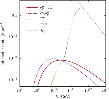
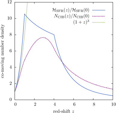
Figure 16: Left: The interaction and decay rates appearing in the Boltzmann equations for the CMB and CIB at $z=0$. Right: Star formation rate (Eq. (111) from Ref. [158]) compared with our approximation (110) for the CIB photon density scaling with redshift. For comparison, the $\propto(1+z)^{3}$ scaling of the CMB photon density is also shown. From Ref.  [157].

The redshift scaling of Eqs. (100) and (101) depend on how the photon backgrounds vary with redshift. The CMB spectral density (GeV^-1 cm^-3) scales adiabatically as:

$$n_{\gamma}(z,\omega)=(1+z)^{2}\,n_{\gamma}(0,\omega/(1+z))\,,$$ (104)

following from $\dot{Y}_{\gamma}=\partial_{E}(HEY_{\gamma})$ and $Y_{\gamma}\propto a^{3}n_{\gamma},$ where $a$ is the cosmic scale factor. The scaling behavior of Eq. (104) translates into the following scaling of the quantities $\Gamma_{i}$ and $\gamma_{ij}$ [21]:

$$\Gamma_{i}(z,E_{i}) = (1+z)^{3}\,\Gamma_{i}(0,(1+z)E_{i})\,,$$ (105)

$$\gamma_{ij}(z,E_{i},E_{j}) = (1+z)^{4}\,\gamma_{ij}(0,(1+z)E_{i},(1+z)E_{j})\,.$$ (106)

The scaling behaviour of $b$ and its derivative $\partial_{E}b$ do again depends on the photon background. For the CMB contribution, we have

$$b_{i}(z,E_{i}) = (1+z)^{2}\,b_{i}(0,(1+z)E_{i})\,,$$ (107)

$$\partial_{E}b_{i}(z,E_{i}) = (1+z)^{3}\,\partial_{E}b_{i}(0,(1+z)E_{i})\,.$$ (108)

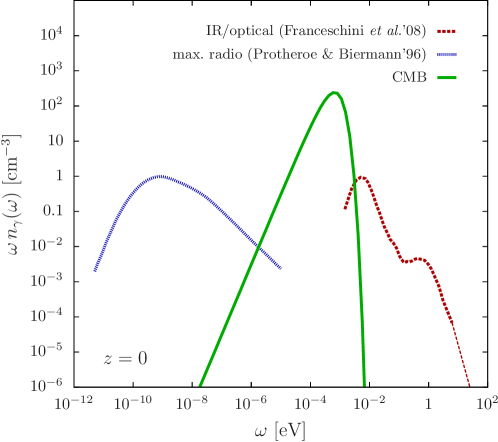
Figure 17: The energy spectrum of the CMB and the CIB in the IR/optial and radio range at $z=0$. The thin dashed line shows our extrapolation to UV energies. From Ref. [160].

We now discuss the red-shift scaling of the quantities $b_{i}$, $\partial_{E}b_{i}$, $\gamma_{ij}$ and $\Gamma_{i}$ for the case of the cosmic infrared background. The CIB spectrum has been studied and tabulated for redshifts up to $z=2$ [159] (which we extrapolate slightly to UV energies as seen in Fig. 17). This is consistent with the constraints on the $\gamma$-ray opacity of the universe set by HESS [161], MAGIC [162] and Fermi-LAT [163] from non-observation of the expected cutoffs in the $\gamma$-ray spectra of extragalactic sources. The redshift dependence is given by:

$$n_{\rm CIB}(z,(1+z)E)=(1+z)^{2}\int_{z}^{\infty}dz^{\prime}\frac{1}{H(z^{\prime})}\mathcal{Q}_{\rm CIB}(z^{\prime},(1+z^{\prime})E)\,,$$ (109)

where $\mathcal{Q}_{\rm CIB}$ is the comoving luminosity density of the sources and we neglect absorption effects other than expansion. We assume that this follows the star formation rate: $\mathcal{Q}_{\rm CIB}(z,E)\propto\mathcal{H}_{\rm SFR}(z)\,\mathcal{Q}_{\rm CIB}(0,E)$. We can then infer the bolometric evolution to be:

$$\frac{N_{\rm CIB}(z)}{N_{\rm CIB}(0)}=(1+z)^{3}\frac{\int_{z}^{\infty}dz^{\prime}\,\mathcal{H}_{\rm SFR}/(H(z^{\prime})(1+z^{\prime}))}{\int_{0}^{\infty}dz^{\prime}\,\mathcal{H}_{\rm SFR}/(H(z^{\prime})(1+z^{\prime}))}\,,$$ (110)

where $N_{\rm CIB}(z)$ is the number of infrared–optical photons per proper volume at redshift $z$. Following a recent compilation [164, 158], we adopt

$$\mathcal{H}_{\rm SFR}(z)=\begin{cases}(1+z)^{3.4}&z<1\,,\\ N_{1}\,(1+z)^{-0.3}&1<z<4\,,\\ N_{1}\,N_{4}\,(1+z)^{-3.5}&z>4\,,\end{cases}$$ (111)

with appropriate normalization factors, $N_{1}=2^{3.7}$ and $N_{4}=5^{3.2}$ (see the right panel of Fig. 16). For comparison, the CMB evolves as $N_{\rm CMB}(z)/N_{\rm CMB}(0)=(1+z)^{3}$. To simplify the numerical evaluation we approximate the evolution with redshift as

$$n_{\rm CIB}(z,\omega)\simeq\frac{1}{1+z}\,\frac{N_{\rm CIB}(z)}{N_{\rm CIB}(0)}\,n_{\rm CIB}(0,\omega/(1+z))\,,$$ (112)

and this is shown in the right panel of Fig. 16. The redshift scaling of the quantities $\gamma_{ij}$, $\Gamma_{i}$, $b_{i}$ and $\partial_{E}b_{i}$ for the CIB is then obtained from the corresponding scaling given for the CMB in Eqs. (105/106) and (107/108), by multiplying the r.h.s. by a factor $N_{\rm CIB}(z)/N_{\rm CIB}(0)/(1+z)^{3}$.

We have little direct knowledge of the cosmic radio background. An estimate made using the RAE satellite [165] is often used to calculate the cascading of UHE photons. A theoretical estimate has been made [166] of the intensity down to kHz frequencies, based on the observed luminosity function and radio spectra of normal galaxies and radio galaxies, although there are large uncertainties in the assumed evolution. The calculated values are about a factor of $\sim 2$ above the measurements and to ensure maximal energy transfer in the cascade we will adopt this estimate and assume the same redshift scaling as the cosmic infrared/optical background. We summarize the adopted cosmic radiation backgrounds in Fig. 17.

The emission rate of CR protons per comoving volume is assumed, as per usual practice, to follow a power-law:

$$\mathcal{Q}_{p}(0,E)\propto(E/E_{0})^{-\gamma}\times\begin{cases}f_{-}(E/E_{\rm min})&E<E_{\rm min}\,,\\ 1&E_{\rm min}<E<E_{\rm max}\,,\\ f_{+}(E/E_{\rm max})&E_{\rm max}<E\,.\end{cases}$$ (113)

We will consider spectral indices $\gamma$ in the range $2\div 3$. The functions $f_{\pm}(x)\equiv x^{\pm 2}\exp(1-x^{\pm 2})$ in Eq. (113) smoothly turn off the contribution below $E_{\rm min}$ and above $E_{\rm max}$. We set $E_{\rm max}=10^{12}$ GeV in the following and vary $E_{\rm min}$ in the range $10^{8.5}\div 10^{10}$ GeV, corresponding to a galactic-extragalactic crossover between the second knee and the ankle in the CR spectrum.

The cosmic evolution of the spectral emission rate per comoving volume is parameterized as:

$$\mathcal{Q}_{p}(z,E)=\mathcal{H}(z)\mathcal{Q}_{p}(0,E)\,.$$ (114)

For simplicity, we use the standard approximation

$$\mathcal{H}(z)\equiv(1+z)^{n}\Theta(z_{\rm max}-z)\,,$$ (115)

with $z_{\rm max}=2$. Note that the dilution of the source density due to the Hubble expansion is taken care of since $\mathcal{Q}$ is the comoving density, i.e. for no evolution we would simply have $\mathcal{H}=1$. We consider cosmic evolution of UHECR sources with $n$ in the range $2\div 6$.

We can express the system of partial integro-differential equations (99) in terms of a system of ordinary integro-differential equations [157],

$$\dot{\mathcal{E}}_{i} =-H\mathcal{E}_{i}-b_{i}(z,\mathcal{E}_{i})\,,$$ (116)

$$\dot{Z}_{i} =\big{[}\beta_{i}(z,\mathcal{E}_{i})-\Gamma_{i}(z,\mathcal{E}_{i})\big{]}\,Z_{i}+(1+z)\mathcal{Q}^{\mathrm{eff}}_{i}(z,\mathcal{E}_{i})\,,$$ (117)

where we have defined $\beta_{i}(z,E)\equiv\partial_{E}b_{i}(z,E)$ and $Z_{i}(z,E)\equiv(1+z)Y_{i}(z,\mathcal{E}_{i}(z,E))$. The quantity $\mathcal{E}_{i}(z,E)$ gives the energy that a particle of type $i$ had at redshift $z$ if we observe it today with energy $E$ and take into account CEL. The effective source term in Eq. (117) is

$$\mathcal{Q}^{\mathrm{eff}}_{i}(z,\mathcal{E}_{i}(z,E))=\mathcal{Q}_{i}+\sum_{j}\int dE\,\,\partial_{E}\mathcal{E}_{j}\,\gamma_{ji}(z,\mathcal{E}_{j},E_{i})\,\frac{Z_{j}}{1+z}\,,$$ (118)

where $\mathcal{E}_{j}(z\,,E)$ and $Z_{j}(z,E)$ are subject to the boundary conditions $\mathcal{E}_{j}(0,E)=E$ and $Z_{j}(z_{\mathrm{max}},E)=0$. The flux at $z=0$ can be expressed as

$$J_{i}(E) = \frac{1}{4\pi}Z_{i}(0,E)$$ (119)

$$= \frac{1}{4\pi}\int_{0}^{\infty}\!\!\!\!\!\!dz\exp\left[\int_{0}^{z}\!\!dz^{\prime}\frac{\partial_{E}b_{i}(z^{\prime},\mathcal{E}_{i}(z^{\prime},E))-\Gamma_{i}(z^{\prime},\mathcal{E}_{i}(z^{\prime},E))}{(1+z^{\prime})H(z^{\prime})}\right]\frac{\mathcal{Q}^{\mathrm{eff}}_{i}(z,\mathcal{E}_{i}(z,E))}{H(z)}.$$

For the numerical evaluation of the Boltzmann equations (99) it is convenient to solve [160]

$$-H(z)(1+z)\partial_{z}{\mathscr{Z}}_{i}(z,E)=-\Gamma(z,{\mathscr{E}}){\mathscr{Z}_{i}}(z,E)+\frac{1}{(1+z)}\partial_{E}[b(z,{\mathscr{E}}){\mathscr{Z}}_{i}(z,E)]+(1+z){\cal Q}_{i}^{\rm eff}(z,{\mathscr{E}})\,.$$ (120)

where we have defined ${\mathscr{E}}=(1+z)E$, and ${\mathscr{Z}}_{i}(z,E)\equiv(1+z)Y_{i}(z,{\mathscr{E}})$, subject to the boundary condition ${\mathscr{Z}}_{j}(z_{\rm max},E)=0$. The effective source term becomes ${\cal Q}_{i}^{\rm eff}(z,{\mathscr{E}})=\mathcal{Q}_{i}+\sum_{j}\int dE_{j}\,\gamma_{ji}(z,{\mathscr{E}}_{j},E_{i})\,{\mathscr{Z}_{j}}$. In our calculation we use logarithmic energy bins with size $\Delta\log_{10}E=0.05$ between $10^{5}$ GeV and $10^{15}$ GeV. For the numerical evolution of the differential Eq. (116) we use a simple Euler method with a step-size $\Delta z=10^{-4}$. The corresponding step-size in the propagation distance $\Delta r=c\Delta t$ is then always smaller than the proton interaction length. The flux at $z=0$ is given by $J_{i}(E)=\mathscr{Z}_{i}(0,E)/(4\pi).$

Electromagnetic (EM) interactions of photons and leptons with the extra-galactic background light and magnetic field can happen on time-scales much shorter than their production rates. It is convenient to account for these contributions during the proton propagation as fast developing electro-magnetic cascades at a fixed redshift. We will use the efficient method of “matrix doubling” [167] for the calculation of the cascades. Since the cascade $\gamma$-ray flux is mainly in the GeV-TeV region and has an almost universal shape here, it is numerically much more efficient to calculate the total energy density $\omega_{\rm cas}$ injected into the cascade and compare this value to the limit imposed by Fermi-LAT. The total energy density (eV cm^-3) of EM radiation from proton propagation in the past is given as

$$\omega_{\rm cas}\equiv\int dEEn_{\rm cas}(0,E)=\int dt\int dE\,\frac{b_{\rm cas}(z,E)}{(1+z)^{4}}\,n_{p}(z,E)\,,$$ (121)

where $n_{p}(z,E)$ is the physical energy density at redshift $z$, defined via $n_{p}(z,E)\equiv(1+z)^{3}Y_{p}(z,E)$; details on the calculation are given in Appendix .6. The continuous energy loss of protons into the cascade, denoted by $b_{\rm cas}$, is in the form of electron, positron and $\gamma$-ray production in BH ($b_{\rm BH}$) and photopion ($b_{\pi}$) interactions. We derive the BH and photopion contribution to $\omega_{\rm cas}$ separately. For the photopion contribution we estimate

$$b_{\pi}(z,E)\simeq\int dE^{\prime}E^{\prime}\left[\gamma_{pe^{-}}(z,E,E^{\prime})+\gamma_{pe^{+}}(z,E,E^{\prime})+\gamma_{p\gamma}(z,E,E^{\prime})\right]\,,$$ (122)

where the angular-averaged distribution of particle $j$ after the interaction are determined using the Monte Carlo package sophia [168]. For the energy loss via BH pair production we use (37). Note, that since the photopion contribution in the cascade is dominated at the GZK cutoff, its contribution should increase relative to BH pair production with increasing crossover energy and, hence, also the associated neutrino fluxes after normalization to $\gamma$-ray and CR data.

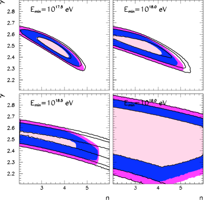
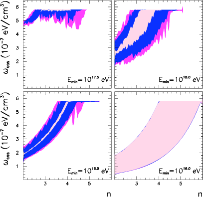
Figure 18: Left Panel: Goodness-of-fit test of the HiRes data [28]. We show the 68% (pink), 95% (blue) and 99% (magenta) confidence levels of the injection index $\gamma$ and the cosmic evolution index $n$. The black lines indicate the allowed regions before the cascade ($\omega_{\rm cas}$) bound is imposed. Right Panel: The corresponding energy density in the EM cascade. From Ref. [160].

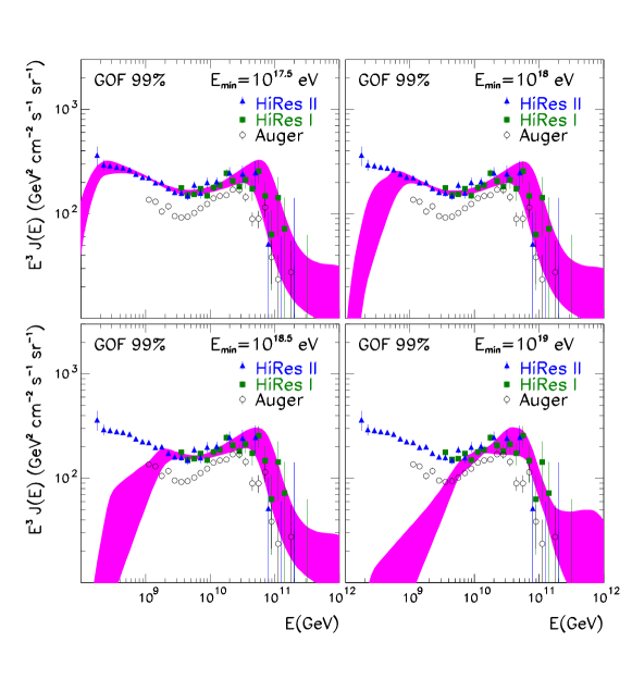
Figure 19: The allowed proton flux (at the 99% confidence level) for increasing crossover energy $E_{\rm min}$. Each fit of the proton spectrum is marginalized with respect to the experimental energy uncertainty and we show the shifted predictions in comparison to the HiRes central values [28]. For comparison we also show the Auger data [29, 30] which has not been included in the fit. From Ref. [160].

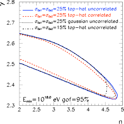
Figure 20: Systematic effect of the experimental energy resolution on the fitted spectral index $\gamma$ and cosmological evolution parameter $n$. For illustration we show the dependence of the 95% C.L. bound for a crossover energy of $10^{18}$ eV. The blue contour corresponds to the region shown in Fig. 18 assuming an uncorrelated energy shift of 25% in both data sets (HiRes I and II) [28], for a flat prior (“top-hat” distribution). The red dashed curve assumes correlated errors of the energy resolution in both data sets. The black dotted curve shows the result for uncorrelated errors with a Gaussian prior, and the dashed-dotted line shows uncorrelated errors with a flat prior, but with a lower uncertainty of 15%. From Ref. [160].

Next, we study the constraint set by the diffuse $\gamma$-ray background on all-proton models of extragalactic CRs. We parametrize our ignorance of the crossover energy – which marks the transition between the galactic and extragalactic components – as a variable low energy cutoff in the proton injection rate. By fitting only to CR data above the crossover energy, taken to be between $10^{8.5}$ GeV and $10^{10}$ GeV, we determine the statistically preferred values of the spectral index $\gamma$, cosmic source density evolution index $n$, and crossover energy $E_{\rm min}$ by a goodness-of-fit (GOF) test of the HiRes data, taking into account the energy resolution of about 25%. For each model we check that the total energy density of the EM cascade is below a critical value inferred from the recent measurement of the extragalactic $\gamma$-ray background by the Fermi-LAT Collaboration [169].

Given the acceptance $A_{i}$ (in units of area per unit time per unit solid angle) of the experiment for the energy bin $i$ centered at $E_{i}$ and with bin width $\Delta_{i}$, and the energy scale uncertainty of the experiment, $\sigma_{E_{s}}$ the number of expected events in the bin is given by

$$N_{i}(n,\gamma,N_{0},\delta)=A_{i}\int_{E_{i}(1+\delta)-\Delta_{i}/2}^{E_{i}(1+\delta)+\Delta_{i}/2}J^{p}_{N_{0},n,\gamma}(E)dE\;,$$ (123)

where

$$J^{p}_{N_{0},n,\gamma}(E)=\frac{c}{4\pi}\ n_{p}(0,E)$$ (124)

is the proton flux arriving at the detector corresponding to a proton source luminosity as in Eq. (113), with the cosmic evolution of the source density given by Eqs. (114) and (115). The parameter $\delta$ in Eq. (123) above is a fractional energy-scale shift that reflects the energy-scale uncertainty of the experiment, and $N_{0}$ is the normalization of the proton source luminosity.

The probability distribution of events in the $i$-th bin is of the Poisson form with mean $N_{i}$. Correspondingly the $r$-dimensional ($r$ being the number of bins of the experiment with $E_{i}\geq E_{\rm min}$) probability distribution for a set of non-negative integer numbers ${\vec{k}}=\{k_{1},...k_{r}\}$, $P_{\vec{k}}(n,\gamma,N_{0},\delta)$, is just the product of the individual Poisson distributions. According to this $r$-dimensional probability distribution, the experimental result ${\vec{N}^{\rm exp}}=\{N^{\rm exp}_{1},...,N^{\rm exp}_{r}\}$ has a probability $P_{\vec{N}^{\rm exp}}(n,\gamma,N_{0},\delta)$ and, correspondingly, the experimental probability after marginalizing over the energy scale uncertainty and normalization is:

$$P_{\rm exp}(n,\gamma)={\rm Max}_{\delta,N_{0}}P_{\vec{N}^{\rm exp}}(n,\gamma,N_{0},\delta)\,,$$ (125)

where the maximization is made within some prior for $\delta$ and $N_{0}$. For the energy shift $\delta$ we have used two forms for the prior, either a top-hat spanning the energy-scale uncertainty of the experiment, $\sigma_{E_{s}}$, or a gaussian prior of width $\sigma_{E_{s}}$.

For $N_{0}$ we impose the prior arising from requiring consistency with the Fermi-LAT measurements [169] of the diffuse extra-galactic $\gamma$-ray background. In order to do so, we obtain the total energy density of EM radiation from the proton propagation using Eq. (121) and we require following Ref. [170]:

$$\omega_{\rm cas}(N_{0},n,\gamma)\leq 5.8\times 10^{-7}\;{\rm eV}/{\rm cm}^{3}\,.$$ (126)

The marginalization in Eq. (125) also determines $N_{0}^{\rm best}$ and $\delta^{\rm best}$ for the model, which are the values of the energy shift and normalization that yield the best description of the experimental CR data, subject to the constraint imposed by the Fermi-LAT measurement.

Altogether the model is compatible with the experimental results at given GOF if

$$\sum_{\vec{k}}P_{\vec{k}}(n,\gamma,N_{0}^{\rm best},\delta^{\rm best})\Theta\left[P_{\vec{k}}(n,\gamma,N_{0}^{\rm best},\delta^{\rm best})-P_{\rm exp}(n,\gamma)\right]\leq{\rm GOF}\,.$$ (127)

Technically, this is computed by generating a large number $N_{\rm rep}$ of replica experiments according to the probability distribution $P_{\vec{k}}(n,\gamma,N_{0}^{\rm best},\delta^{\rm best})$ and imposing the fraction $F$ of those which satisfy $P_{\vec{k}}(n,\gamma,N_{0},\delta^{\rm best})>P_{\rm exp}(n,\gamma)$ to be $F\leq{\rm GOF}$.

Table 3: Cosmic ray source parameters which best fit the HiRes data [28], along with those which yield minimal and maximal contributions to $\omega_{\pi}$ (i.e. neutrino fluxes) and $\omega_{\mathrm{cas}}=\omega_{\pi}+\omega_{\mathrm{BH}}$ (i.e. $\gamma$-ray fluxes), all at the 99% C.L.

	$E_{\rm min}=10^{8.5}$ GeV					$E_{\rm min}=10^{9}$ GeV
model	$n$	$\gamma$	$\omega_{\rm cas}$a	$\delta_{I\rm best}$	$\delta_{II\rm best}$	$n$	$\gamma$	$\omega_{\rm cas}$a	$\delta_{I\rm best}$	$\delta_{II\rm best}$
	fit with Fermi-LAT bound:
best fit	$3.50$	$2.49$	$5.8$	0.005	0.	$3.20$	$2.52$	$5.2$	0.050	0.045
min. $\omega_{\rm cas}$	$4.50$	$2.31$	$4.4$	-0.235	-0.245	$2.25$	$2.47$	$1.7$	-0.120	-0.150
max. $\omega_{\rm cas}$	$4.60$	$2.36$	$5.8$	-0.185	-0.175	$3.35$	$2.55$	$5.8$	0.050	0.060
min. $\omega_{\pi}$	$2.00$	$2.67$	$4.9$	0.215	0.235	$2.00$	$2.51$	$1.8$	-0.070	-0.095
max. $\omega_{\pi}$	$4.80$	$2.29$	$5.8$	-0.220	-0.215	$5.10$	$2.29$	$5.8$	-0.250	-0.250
	fit without Fermi-LAT bound:
max. $\omega_{\rm cas}$	$4.45$	$2.44$	$15$	0.135	0.155	$5.25$	$2.36$	$27$	0.205	0.205
max. $\omega_{\pi}$	$4.80$	$2.36$	$14$	0.050	0.055	$5.30$	$2.35$	$26$	0.190	0.190
	$E_{\rm min}=10^{9.5}$ GeV					$E_{\rm min}=10^{10}$ GeV
model	$n$	$\gamma$	$\omega_{\rm cas}$a	$\delta_{I\rm best}$	$\delta_{II\rm best}$	$n$	$\gamma$	$\omega_{\rm cas}$a	$\delta_{I\rm best}$	$\delta_{II\rm best}$
	fit with Fermi-LAT bound:
best fit	$4.05$	$2.47$	$5.8$	0.015	0.005	$4.60$	$2.50$	$4.4$	-0.030	-0.065
min. $\omega_{\rm cas}$	$2.00$	$2.45$	$1.4$	-0.050	-0.060	$2.00$	$2.88$	$0.44$	-0.220	-0.250
max. $\omega_{\rm cas}$	$4.95$	$2.37$	$5.8$	-0.165	-0.160	$4.45$	$2.13$	$5.8$	0.130	0.090
min. $\omega_{\pi}$	$2.00$	$2.63$	$2.1$	0.075	0.070	$2.00$	$2.88$	0.44	-0.220	-0.250
max. $\omega_{\pi}$	$5.35$	$2.28$	$5.8$	-0.240	-0.250	$4.40$	$2.10$	$5.8$	0.145	0.100
	fit without Fermi-LAT bound:
max. $\omega_{\rm cas}$	$6.00$	$2.49$	$30$	0.120	0.135	$6.00$	$2.14$	$23$	0.250	0.210
max. $\omega_{\pi}$	$6.00$	$2.47$	$29$	0.120	0.125	$6.00$	$2.10$	$23$	0.250	0.210

With this method we determine the value of $(n,\gamma)$ parameters that are compatible with the HiRes I and HiRes II experiments [28]. In the left panel of Fig. 18, we plot the regions with GOF 64%, 95% and 99% for four values of the minimum (i.e. crossover) energy. In the right panel, we show the corresponding ranges of $\omega_{\rm cas,best}$ for the models as a function of the cosmic evolution index $n$. In order to display explicitly the impact of the constraint from the Fermi-LAT measurements of the diffuse extra-galactic $\gamma$-ray background (126), we show the corresponding GOF regions without imposing that constraint. In Table. 3 we list the parameters corresponding to the best-fit models and to the models with minimal and maximal contributions to $\omega_{\pi}$ and $\omega_{\rm cas}=\omega_{\pi}+\omega_{\rm BH}$ at the 99% C.L., together with the corresponding energy shifts which give best fits to the HiRes I and HiRes II data. We also show the parameters for the models with maximum $\omega_{\pi}$ and $\omega_{\rm cas}$ without imposition of the Fermi-LAT constraint.

It is interesting to compare the allowed values of $n$ with those in the cosmological evolution of UHECR candidate sources. For GRBs [171],

$$\mathcal{H}_{\rm GRB}(z)=(1+z)^{1.4}\,\mathcal{H}_{\rm SFR}(z)\,,$$ (128)

for AGNs [173, 172]

$$\mathcal{H}_{\rm AGN}(z)=\begin{cases}(1+z)^{5.0}&z<1.7\,,\\ N_{1.7}&1.7<z<2.7\,,\\ N_{1.7}\,N_{2.7}^{(2.7-z)}&z>2.7\,,\end{cases}$$ (129)

with $N_{1.7}=2.7^{5}$ and $N_{2.7}=10^{0.43}$, and for QSO [174]

$$\mathcal{H}_{\rm QSO}(z)=\begin{cases}(1+z)^{3}&z<1.9\,,\\ (1+1.9)^{3}&1.9<z<2.7\,,\\ (1+1.9)^{3}\exp\{(2.7-z)/2.7\}\,,&z>2.7\,.\end{cases}$$ (130)

As an illustration of the agreement with the CR data, in Fig. 18 we show the range of proton fluxes corresponding to models with GOF 99% or better for increasing crossover energies $E_{\rm min}$. As discussed above, each fit of the proton spectra is marginalized with respect to the experimental energy scale uncertainty and we show the shifted predictions with $\delta^{\rm best}$ in comparison to the HiRes data at central value. In the figure we also show the results from Auger [29, 30], though these have not been included in the analysis.

These results are obtained assuming an energy scale uncertainty $\sigma_{E_{s}}=5\%$ with a “top-hat” prior for the corresponding energy shifts which are taken to be uncorrelated for HiRes I and HiRes II. In Fig. 20 we explore the dependence of the results on these assumptions by using a different form for the prior, assuming the energy shifts to be correlated between the two experiments, or reducing the uncertainty to $\sigma_{E_{s}}=15\%$. As seen in the figure, the main effect is associated with the reduction of the energy scale uncertainty which, as expected, results in a worsening of the GOF for models with larger $n$. This is directly related to the normalization constraint from Eq. (126). If one naively ignores the energy scale uncertainty, the constraint in Eq. (126) rules out models with $n\gtrsim 3$ (the precise value depending on the assumed $E_{\rm min}$). However, once the energy scale uncertainty is included, the constraint of Eq. (126) plays a weaker role on the determination of the GOF of the models. It does, however, imply a maximum value of $N_{0}^{\rm best}$ which, as we will see, impacts the corresponding ranges of neutrino fluxes.

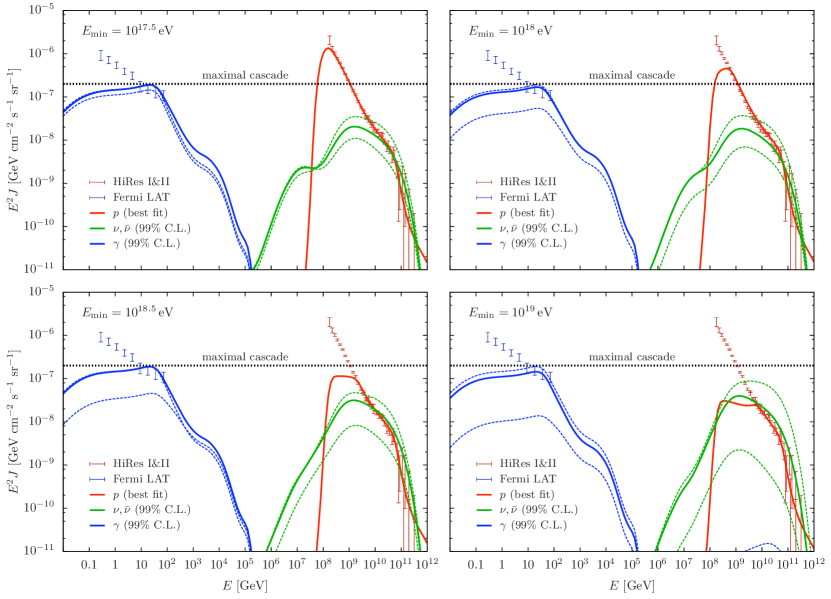
Figure 21: Comparison of proton, neutrino and $\gamma$-ray fluxes for different crossover energies. We show the best-fit values (solid lines) as well as neutrino and $\gamma$-ray fluxes within the 99% C.L. with minimal and maximal energy density (dashed lines). The values of the corresponding model parameters can be found in Table. 3. The dotted line labeled “maximal cascade” indicates the approximate limit $E^{2}J_{\rm cas}\lesssim c\,\omega_{\rm cas}^{\rm max}/4\pi\log({\rm TeV}/{\rm GeV})$, corresponding to a $\gamma$-ray flux in the GeV-TeV range saturating the energy density (126). The $\gamma$-ray fluxes are marginally consistent at the 99% C.L. with the highest energy measurements by Fermi-LAT. The contribution around 100 GeV is somewhat uncertain due to uncertainties in the cosmic infrared background. From Ref. [160].

The corresponding range of $\gamma$-ray and cosmogenic neutrino fluxes (summed over flavor) is shown in Fig. 21 for models with minimal and maximal energy density at the 99% C.L. As expected, the maximum $\gamma$-ray fluxes are consistent with the Fermi-LAT data within the errors. For illustration, we also show as a dotted line the “naive” $\gamma$-ray limit $E^{2}J_{\rm cas}\lesssim c\,\omega_{\rm cas}^{\rm max}/4\pi\log({\rm TeV}/{\rm GeV})$, corresponding to a $\gamma$-ray flux in the GeV-TeV range which saturates the energy density (126).

The cosmogenic neutrino and photon fluxes are also sensitive to the primary composition. For example, if the primaries are iron nuclei one would expect a considerably lower flux on both photons and neutrinos, rendering photon pile-up measurements less helpful in constraining cosmogenic fluxes. (See Appendix .5 for details).

Upper limits on the cosmic neutrino flux

High energy neutrino detection is one of the experimental challenges in particle astrophysics for the forthcoming years. It is widely believed that one of the most appropriate techniques for neutrino detection consists of detecting the Cherenkov light from muons or showers produced by the neutrino interactions in underground water or ice. For a recent review see e.g. [175]. This allows instrumentation of large enough volumes to compensate for both the low neutrino cross section and the low fluxes expected. There are several projects under way to build sufficiently large detectors to measure the expected signals from a variety of neutrino sources. The IceCube facility, deployed near the Amundsen-Scott station, is the largest neutrino telescope in the world [176]. It comprises a cubic-kilometer of ultra-clear ice about a mile below the South Pole surface, instrumented with long strings of sensitive photon detectors which record light produced when neutrinos interact in the ice.

CR experiments, like Auger, provide a complementary technique for UHEC$\nu$ detection by searching for deeply–developing, large zenith angle ($>75^{\circ}$) showers [177]. At these large angles, hadron-induced showers traverse the equivalent of several atmospheres before reaching detectors at the ground. Beyond about 2 atmospheres, most of the electromagnetic component of a shower is extinguished and only very high energy muons survive. Consequently, a hadron-induced shower front is relatively flat and the shower particles arrive within a narrow time window (Fig. 22, top panel). In contrast, a neutrino shower exhibits characteristics similar to those of a vertical shower, which has a more curved front and a wider distribution in particle arrival times due to the large number of lower energy electrons and photons. Furthermore, the “early” part of the shower will tend to be dominated by the electromagnetic component, while “late” portion will be enriched with tightly bunched muons (Fig. 22, middle panel). Using these characteristic features, it is possible to distinguish neutrino induced events from background hadronic showers. Moreover, because of full flavor mixing, tau neutrinos are expected to be as abundant as other species in the cosmic flux. Tau neutrinos can interact in the Earth’s crust, producing $\tau$ leptons which may decay above the Auger detectors [179, 178, 180] (Fig. 22, bottom panel). Details on how such events can be selected at the Auger Observatory are discussed in  [181, 182].

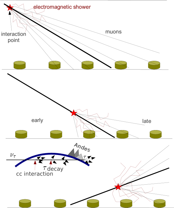
Figure 22: Schematic illustration of the properties of a hadron-induced shower (top), an $\nu$-induced nearly horizontal shower (middle) and a $\nu_{\tau}$-induced earth skimming shower (bottom). Note that only up-going showers resulting from $\tau$ neutrino interactions in the Earth can be detected with any efficiency using the surface array. In contrast, all three neutrino species can be detected in down-going showers. Also note from the inset in the lower panel, that the incident $\tau$ can experience several CC interactions and decays and thereby undergo a regeneration process. The Andes mountain range lies to the west of the observatory, and provides roughly an additional 20% target volume for $\nu_{\tau}$ interactions.

So far, no neutrino candidates have been observed resulting in upper limits on the diffuse flux of neutrinos. For the case of up-going $\tau$ neutrinos in the energy range $2\times 10^{8}\leavevmode\nobreak\ {\rm GeV}<E_{\nu}<2\times 10^{10}\leavevmode\nobreak\ {\rm GeV}$, assuming a diffuse spectrum of the form $E_{\nu}^{-2}$, the current 90%CL bound, is [183]

$$E_{\nu}^{2}\ \Phi^{\nu_{\tau}}\simeq 4.7^{-2.5}_{+2.2}\times 10^{-8}\leavevmode\nobreak\ {\rm GeV}\leavevmode\nobreak\ {\rm cm}^{-2}\leavevmode\nobreak\ {\rm s}^{-1}\leavevmode\nobreak\ {\rm sr}^{-1}\,.$$ (131)

Though Auger was not designed specifically as a neutrino detector, it is interesting to note that it exhibits good sensitivity in an energy regime complementary to those available to other dedicated instruments. For example, the 90% CL upper limit from IceCube, for neutrinos of all flavors in the energy range $2.0\times 10^{6}\leavevmode\nobreak\ {\rm GeV}<E_{\nu}<6.3\times 10^{9}\leavevmode\nobreak\ {\rm GeV}$, is [184]

$$E_{\nu}^{2}\ \Phi^{\nu_{\rm all}}\simeq 3.6\times 10^{-8}\leavevmode\nobreak\ {\rm GeV}\leavevmode\nobreak\ {\rm cm}^{-2}\leavevmode\nobreak\ {\rm s}^{-1}\leavevmode\nobreak\ {\rm sr}^{-1}\,.$$ (132)

We now derive model-independent bounds on the total neutrino flux. The event rate for quasi-horizontal deep showers is

$$N=\sum_{i,X}\int dE_{i}\,N_{A}\,\Phi^{i}(E_{i})\,\sigma_{iN\to X}(E_{i})\,{\cal E}(E_{i})\ ,$$ (133)

where the sum is over all neutrino species $i=\nu_{e},\bar{\nu}_{e},\nu_{\mu},\bar{\nu}_{\mu},\nu_{\tau},\bar{\nu}_{\tau}$, and all final states $X$. $N_{A}=6.022\times 10^{23}$ is Avogadro’s number, and $\Phi^{i}$ is the source flux of neutrino species $i$, $\sigma$ as usual denotes the cross section, and ${\cal E}$ is the exposure measured in cm³ w.e. sr time. The Pierre Auger Collaboration has searched for quasi-horizontal showers that are deeply-penetrating [183]. There are no events that unambiguously pass all the experimental cuts, with zero events expected from hadronic background. This implies an upper bound of 2.4 events at 90%CL from neutrino fluxes [185]. Note that if the number of events integrated over energy is bounded by 2.4, then it is certainly true bin by bin in energy. Thus, using Eq. (133) one obtains

$$\sum_{i,X}\int_{\Delta}dE_{i}\,N_{A}\,\Phi^{i}(E_{i})\,\sigma_{iN\to X}(E_{i})\,{\cal E}(E_{i})\ <2.4\ ,$$ (134)

at 90% CL for some interval $\Delta$. Here, the sum over $X$ takes into account charge and neutral current processes. In a logarithmic interval $\Delta$ where a single power law approximation

$$\Phi^{i}(E_{i})\,\sigma_{iN\to X}(E_{i})\,{\cal E}(E_{i})\sim E_{i}^{\alpha}$$ (135)

is valid, a straightforward calculation shows that

$$\int_{\langle E\rangle e^{-\Delta/2}}^{\langle E\rangle e^{\Delta/2}}\frac{dE_{i}}{E_{i}}\,E_{i}\,\Phi^{i}\,\sigma_{iN\to X}\,{\cal E}=\langle\sigma_{iN\rightarrow X}\,{\cal E}\,E_{i}\,\Phi^{i}\rangle\,\frac{\sinh\delta}{\delta}\,\Delta\,,$$ (136)

where $\delta=(\alpha+1)\Delta/2$ and $\langle A\rangle$ denotes the quantity $A$ evaluated at the center of the logarithmic interval [186]. The parameter $\alpha=0.363+\beta-\gamma$, where 0.363 is the power law index of the SM neutrino cross section [187] and $\beta$ and $-\gamma$ are the power law indices (in the interval $\Delta$) of the exposure and flux $\Phi^{i}$, respectively. Since $\sinh\delta/\delta>1$, a conservative bound may be obtained from Eqs. (134) and (136):

$$N_{A}\,\sum_{i,X}\langle\sigma_{iN\rightarrow X}(E_{i})\rangle\,\langle{\cal E}(E_{i})\rangle\,\langle E_{i}\Phi^{i}\rangle<2.4/\Delta\ .$$ (137)

By taking $\Delta=1$ as a likely interval in which the single power law behavior is valid (this corresponds to one $e$-folding of energy), it is straightforward to obtain upper limits on the neutrino flux. The model-independent upper limits on the total neutrino flux, derived using an equivalent of 0.8 yr of full Auger exposure, are collected in Table LABEL:tableMI [183].

Table 4: Model-independent upper limits on the neutrino flux at 90% CL.

$E_{\nu}$ (GeV)		$\langle E_{\nu}\ \Phi^{\nu_{\rm all}}\rangle$ (cm-2 sr-1 s${}^{-1})$
$1\times 10^{8}$		$4.3\times 10^{-14}$
$3\times 10^{8}$		$5.3\times 10^{-15}$
$1\times 10^{9}$		$1.2\times 10^{-15}$
$3\times 10^{9}$		$4.7\times 10^{-16}$
$1\times 10^{10}$		$2.2\times 10^{-16}$
$3\times 10^{10}$		$1.3\times 10^{-16}$
$1\times 10^{11}$		$7.2\times 10^{-17}$
$3\times 10^{11}$		$4.3\times 10^{-17}$

0.3 Phenomenology of extensive air showers

0.3.1 Systematic uncertainties in air shower measurements from hadronic interaction models

Uncertainties in hadronic interactions at ultrahigh energies constitute one of the most problematic sources of systematic error in the analysis of air showers. This section will explain the two principal schools of thought for extrapolating collider data to ultrahigh energies.

Soft multiparticle production with small transverse momenta with respect to the collision axis is a dominant feature of most hadronic events at c.m. energies $10\leavevmode\nobreak\ {\rm GeV}<\sqrt{s}<62\leavevmode\nobreak\ {\rm GeV}$ (see e.g., [188, 189]). Despite the fact that strict calculations based on ordinary QCD perturbation theory are not feasible, there are some phenomenological models that successfully take into account the main properties of the soft diffractive processes. These models, inspired by $1/N$ QCD expansion are also supplemented with generally accepted theoretical principles like duality, unitarity, Regge behavior, and parton structure. The interactions are no longer described by single particle exchange, but by highly complicated modes known as Reggeons. Up to about 62 GeV, the slow growth of the cross section with $\sqrt{s}$ is driven by a dominant contribution of a special Reggeon, the Pomeron.

At higher energies, semihard (SH) interactions arising from the hard scattering of partons that carry only a very small fraction of the momenta of their parent hadrons can compete successfully with soft processes [190, 191, 192, 193, 194, 195, 196, 197]. These semihard interactions lead to the “minijet” phenomenon, i.e. jets with transverse energy ($E_{T}=|p_{{}_{T}}|$) much smaller than the total c.m. energy. Such low-$p_{{}_{T}}$ processes cannot be identified by jet finding algorithms, but (unlike soft processes) still they can be calculated using perturbative QCD. The cross section for SH interactions is described by

$$\sigma_{\rm QCD}(s,p_{{{}_{T}}}^{\rm min})=\sum_{i,j}\int\frac{dx_{1}}{x_{1}}\,\int\frac{dx_{2}}{x_{2}}\,\int_{Q_{\rm min}^{2}}^{\hat{s}/2}\,d|\hat{t}|\,\,\frac{d\hat{\sigma}_{ij}}{d|\hat{t}|}\,\,x_{1}f_{i}(x_{1},|\hat{t}|)\,\,\,x_{2}f_{j}(x_{2},|\hat{t}|)\,\,\,,$$ (138)

where $x_{1}$ and $x_{2}$ are the fractions of the momenta of the parent hadrons carried by the partons which collide, $d\hat{\sigma}_{ij}/d|\hat{t}|$ is the cross section for scattering of partons of types $i$ and $j$ according to elementary QCD diagrams, $f_{i}$ and $f_{j}$ are parton distribution functions (PDFs), $\hat{s}=x_{1}\,x_{2}s$ and $-\hat{t}=\hat{s}\,(1-\cos\vartheta^{*})/2=Q^{2}$ are the Mandelstam variables for this parton-parton process, and the sum is over all parton species. Here,

$$p_{{}_{T}}=E_{\rm jet}^{\rm lab}\,\,\sin\vartheta_{\rm jet}=\frac{\sqrt{\hat{s}}}{2}\,\,\sin\vartheta^{*}\,,$$ (139)

and

$$p_{{}_{\parallel}}=E_{\rm jet}^{\rm lab}\,\,\cos\vartheta_{\rm jet}\,,$$ (140)

where $E_{\rm jet}^{\rm lab}$ is the energy of the jet in the lab frame, $\vartheta_{\rm jet}$ the angle of the jet with respect to the beam direction in the lab frame, and $\vartheta^{*}$ is the angle of the jet with respect to the beam direction in the c.m. frame of the elastic parton-parton collision. This implies that for small $\vartheta^{*},$ $p_{{}_{T}}^{2}\approx Q^{2}$. The integration limits satisfy

$$Q_{\rm min}^{2}<|\hat{t}|<\hat{s}/2\,,$$ (141)

where $Q_{\rm min}=1-2\leavevmode\nobreak\ {\rm GeV}$ is the minimal momentum transfer. The measured minijet cross sections indicate that the onset of SH interactions has just occurred by CERN SPS energies ($\sqrt{s}>200\leavevmode\nobreak\ {\rm GeV}$ [198].

A first source of uncertainty in modeling cosmic ray interactions at ultrahigh energy is encoded in the extrapolation of the measured parton densities several orders of magnitude down to low $x$. Primary protons that impact on the upper atmosphere with energy $\sim 10^{11}$ GeV yield partons with $x\equiv 2p^{*}_{{}_{\parallel}}/\sqrt{s}\sim m_{\pi}/\sqrt{s}\sim 10^{-7},$ whereas current data on quark and gluon densities are only available for $x\gtrsim 10^{-4}$ to within an experimental accuracy of 3% for $Q^{2}\approx 20$ GeV² [199]. In Fig. 23 we show the region of the $x-Q^{2}$ plane probed by H1, ZEUS, and fixed target experiments. In addition, extrapolation of HERA data to UHECR interactions assumes universality of the PDFs. This assumption, based on the QCD factorization conjecture (the cross section of Eq. (138) can always be written in a form which factorizes the parton densities and the hard interaction processes irrespective of the order in perturbation theory and the particular hard process) holds in the limit $Q^{2}\gg\Lambda_{\rm QCD}$, where $\Lambda_{\rm QCD}\sim 200$ MeV is the QCD renormalization scale.

Figure 23: Kinematic $x$-$Q^{2}$ plane accessible to the H1 and ZEUS experiments at HERA and the region accessible to fixed-target experiments. The inelasticity $y=(1-\cos\vartheta^{*})/2$ is also shown. From Ref. [200].

For large $Q^{2}$ and not too small $x$, the Dokshitzer-Gribov-Lipatov-Altarelli-Parisi (DGLAP) equations [201, 202, 203, 204]

$$\frac{\partial}{\partial\ln Q^{2}}{q(x,Q^{2})\choose g(x,Q^{2})}=\frac{\alpha_{s}(Q^{2})}{2\pi}{P_{qq}\,\,\,\,P_{qg}\choose P_{gq}\,\,\,\,P_{gg}}\otimes{q(x,Q^{2})\choose g(x,Q^{2})}$$ (142)

successfully predict the $Q^{2}$ dependence of the quark and gluon densities ($q$ and $g,$ respectively). Here, $\alpha_{s}=g^{2}/(4\pi),$ with $g$ the strong coupling constant. The splitting functions $P_{ij}$ indicate the probability of finding a daughter parton $i$ in the parent parton $j$ with a given fraction of parton $j$ momentum. This probability will depend on the number of splittings allowed in the approximation. In the double-leading-logarithmic approximation, that is $\lim_{x\to 0}\ln(1/x)$ and $\lim_{Q^{2}\to\infty}\ln(Q^{2}/\Lambda_{\rm QCD})$, the DGLAP equations predict a steeply rising gluon density, $xg\sim x^{-0.4},$ which dominates the quark density at low $x$. This prediction is in agreement with the experimental results from HERA shown in Fig. 24 [206, 207]. HERA data are found to be consistent with a power law, $xg(x,Q^{2})\sim x^{-\Delta_{\rm H}},$ with an exponent $\Delta_{\rm H}$ between 0.3 and 0.4 [208].

Figure 24: Gluon momentum distributions $xg(x,Q^{2})$ in the proton as measured by the ZEUS and H1 experiments at various $Q^{2}$. From Ref. [205].

The high energy minijet cross section is then determined by the dominant gluon distribution

$$\sigma_{\rm QCD}(s,p_{{{}_{T}}}^{\rm min})\approx\int\frac{dx_{1}}{x_{1}}\,\int\frac{dx_{2}}{x_{2}}\,\int_{Q_{\rm min}^{2}}^{\hat{s}/2}\,d|\hat{t}|\,\,\,\frac{d\hat{\sigma}}{d|\hat{t}|}\,\,\,x_{1}g(x_{1},|\hat{t}|)\,\,\,x_{2}g(x_{2},|\hat{t}|)\,\,,$$ (143)

where the integration limits satisfy

$$x_{1}x_{2}s>2|\hat{t}|>2Q^{2}_{\rm min}\,.$$ (144)

Furthermore, because $d\hat{\sigma}/d|\hat{t}|$ is peaked at the low end of the $|\hat{t}|$ integration (see e.g [209]), the high energy behavior of $\sigma_{\rm QCD}$ is controlled (via the lower limits of the $x_{1},\,x_{2}$ integrations) by the small-$x$ behavior of the gluons [210]

$$\sigma_{\rm QCD}(s)\propto\int_{2\,Q_{\rm min}^{2}/s}^{1}\frac{dx_{1}}{x_{1}}\,\,x_{1}^{-\Delta_{\rm H}}\,\int_{2\,Q_{\rm min}^{2}/x_{1}s}^{1}\frac{dx_{2}}{x_{2}}\,\,x_{2}^{-\Delta_{\rm H}}\sim s^{\Delta_{\rm H}}\,\ln s\,\sim_{{}_{\!\!\!\!\!\!\!\!\!\!s\to\infty}}s^{\Delta_{\rm H}}\,.$$ (145)

This estimate is, of course, too simplistic. At sufficiently small $x$, gluon shadowing corrections suppress the singular $x^{-\Delta_{H}}$ behavior of $xg$ and hence suppress the power growth of $\sigma_{\rm QCD}$ with increasing $s$.

Although we have shown that the onset of semihard processes is an unambiguous prediction of QCD, in practice it is difficult to isolate these contributions from the soft interactions. Experimental evidence indicates that SH interactions can essentially be neglected up to and throughout the CERN ISR energy regime, $\sqrt{s}<62\leavevmode\nobreak\ {\rm GeV}$. Therefore, measurements made in this energy region can be used to model the soft interactions. A reasonable approach introduced in [211] is to base the extrapolation of the soft interactions on the assumption of geometrical scaling [212], which is observed to be true throughout the ISR energy range [213, 214]. To this end, we introduce the standard partial-wave amplitude in impact-parameter space $f(s,b)$, which is the Fourier transform of the elastic $pp$ (or $p\bar{p}$) scattering amplitude. (We neglect any difference between $pp$ and $p\bar{p}$ for $\sqrt{s}>200\leavevmode\nobreak\ {\rm GeV}$.) Geometrical scaling (GS) corresponds to the assumption that $f$, which a priori is a function of two dimensional variables $b$ and $s$, depends only upon one dimensional variable $\beta=b/R(s)$, where $R$ is the energy dependent radius of the proton, i.e.

$$f(s,b)=f_{\rm GS}\left(\beta=b/R(s)\right)\,.$$ (146)

Physically, this means that the opaqueness of the proton remains constant with rising energy and that the increase of the total cross section, $\sigma_{\rm tot}$, in the ISR energy range reflects a steady growth of the radius $R(s)$. An immediate obvious consequence of GS is that the partial wave at $b=0$ should be independent of energy

$$f(s,b=0)=f_{\rm GS}(\beta=0)\,.$$ (147)

Another consequence is that the ratio of elastic scattering to total cross section, $\sigma_{\rm el}(s)/\sigma_{\rm tot}(s)$, should be energy independent. This follows from

$$\sigma_{\rm tot} = 8\pi\int{\rm Im}f(s,b)\,b\,db$$

$$= 8\pi R^{2}(s)\,\int{\rm Im}f_{\rm GS}(\beta)\,\beta\,d\beta,$$

^GS

and

$$\sigma_{\rm el} = 8\pi\int\left|f(s,b)\right|^{2}\,b\,db$$

$$= 8\pi R^{2}(s)\,\int\left|f_{\rm GS}(\beta)\right|^{2}\,\beta\,d\beta\,.$$

^GS

To determine the gross features at high energies we can assume that the elastic amplitude has a simple form

$$F(s,t)=i\ \sigma_{\rm tot}(s)\ \ e^{Bt/2}\,,$$ (150)

with $B$ the slope parameter that measures the size of the proton [215]. This is a reasonable assumption: the amplitude is predominantly imaginary, and the exponential behavior observed for $|t|\lesssim 0.5\leavevmode\nobreak\ {\rm GeV}^{2}$ gives the bulk of the elastic cross section. Now, the Fourier transform $f(s,b)$ of the elastic amplitude $F(s,t)$ given by (150) has a Gaussian form in impact parameter space

$$f(s,b)=\frac{i\sigma_{\rm tot}(s)}{8\pi B}e^{-b^{2}/2B}\,,$$ (151)

and it follows that

$${\rm Im}f(s,b=0)=\frac{\sigma_{\rm tot}}{8\pi B}=\frac{2\sigma_{\rm el}}{\sigma_{\rm tot}}\,.$$ (152)

Equation (152) offers a very clear way to see the breakdown of GS and to identify semihard interactions from the growth of the central partial wave.

In general unitarity requires ${\rm Im}f(s,b)\leq\frac{1}{2}$, which in turm implies $\sigma_{\rm el}/\sigma_{\rm tot}\leq\frac{1}{2}$ [215]. This seems to indicate that the Gaussian form (151) may not longer be applicable at ultrahigh energies, but rather it is expected that the proton will approximate a “black disk” of radius $b_{0}$, i.e. $f(s,b)=\frac{i}{2}$ for $0<b\lesssim b_{0}$ and zero for $b\gtrsim b_{0}$. Then $\sigma_{\rm el}\simeq\frac{1}{2}\sigma_{\rm tot}\simeq\pi b_{0}^{2}$.

In order to satisfy the unitarity constraints, it is convenient to introduce the eikonal $\chi$ defined by

$$f(s,b)=\frac{i}{2}\left\{1-{\rm exp}\left[i\chi(s,b)\right]\right\}\,,$$ (153)

where ${\rm Im}\,\chi\geq 0$. If we neglect for the moment the shadowing corrections to the PDFs and take $xg\propto x^{-\Delta_{\rm H}}$ in the small-$x$ limit we obtain, as explained above, power growth of the cross section for SH interactions, $\sigma_{\rm QCD}\sim s^{\Delta_{\rm H}}$ and ${\rm Im}\chi(s,b=0)\gg 1$ as $s\to\infty$. Indeed we expect ${\rm Im}\,\chi\gg 1$ (and unitarity to be saturated) for a range of $b$ about $b=0$. Then we have

$$\sigma_{\rm tot} = 4\pi\int_{0}^{\infty}b\ db\,\Theta(b_{0}-b)$$ (154)

$$\simeq 4\pi\int_{0}^{b_{0}(s)}b\,db=2\pi b_{0}^{2}\,,$$

with $\chi\simeq\chi_{{}_{\rm SH}}$ and where $b_{0}(s)$ is such that

$${\rm Im}\,\chi_{{}_{\rm SH}}(s,b_{0}(s))\simeq 1\,.$$ (155)

Hereafter, we ignore the small real part of the scattering amplitude, which is good approximation at high energies. The unitarized elastic, inelastic, and total cross sections (considering now a real eikonal function) are given by [216, 217, 218, 219]

$$\sigma_{\rm el}=2\pi\int db\,b\ \left\{1-\exp\left[-\chi_{{}_{\rm soft}}(s,b)-\chi_{{}_{\rm SH}}(s,b)\right]\right\}^{2}\ \,,$$ (156)

$$\sigma_{\rm inel}=2\pi\int db\,b\,\left\{1-\exp\left[-2\chi_{{}_{\rm soft}}(s,b)-2\chi_{{}_{\rm SH}}(s,b)\right]\right\}\ ,$$ (157)

$$\sigma_{\rm tot}=4\pi\int db\,b\,\left\{1-\exp\left[-\chi_{{}_{\rm soft}}(s,b)-\chi_{{}_{\rm SH}}(s,b)\right]\right\}\ ,$$ (158)

where the scattering is compounded as a sum of QCD ladders via SH and soft processes through the eikonals $\chi_{{}_{\rm SH}}$ and $\chi_{{}_{\rm soft}}$.

Now, if the eikonal function, $\chi(s,b)\equiv\chi_{{}_{\rm soft}}(s,b)+\chi_{{}_{\rm SH}}(s,b)=\lambda/2,$ indicates the mean number of partonic interaction pairs at impact parameter $b,$ the probability $p_{n}$ for having $n$ independent partonic interactions using Poisson statistics reads, $p_{n}=(\lambda^{n}/n!)\,e^{-\lambda}$. Therefore, the factor $1-e^{-2\chi}=\sum_{n=1}^{\infty}p_{n}$ in Eq. (157) can be interpreted semiclassically as the probability that at least 1 of the 2 protons is broken up in a collision at impact parameter $b$. With this in mind, the inelastic cross section is simply the integral over all collision impact parameters of the probability of having at least 1 interaction, yielding a mean minijet multiplicity of $\langle n_{\rm minijet}\rangle\approx\sigma_{\rm QCD}/\sigma_{\rm inel}$ [220]. The leading contenders to approximate the (unknown) cross sections at cosmic ray energies, sibyll [221] and qgsjet [222], share the eikonal approximation but differ in their ansätse for the eikonals. In both cases, the core of dominant scattering at very high energies is the SH cross section given in Eq. (138),

$$\chi_{{}_{\rm SH}}=\frac{1}{2}\,\sigma_{\rm QCD}(s,p_{{{}_{T}}}^{\rm min})\,\,A(s,\vec{b})\,,$$ (159)

where the normalized profile function, $2\pi\int_{0}^{\infty}db\,b\,A(s,b)=1,$ indicates the distribution of partons in the plane transverse to the collision axis.

In the qgsjet-like models, the core of the SH eikonal is dressed with a soft-pomeron pre-evolution factor. This amounts to taking a parton distribution which is Gaussian in the transverse coordinate distance $b,$

$$A(s,b)=\frac{e^{-b^{2}/R^{2}(s)}}{\pi R^{2}(s)}\,,$$ (160)

with $R$ being a parameter. For a QCD cross section dependence, $\sigma_{\rm QCD}\sim s^{\Delta_{\rm H}},$ one gets for a Gaussian profile

$$b_{0}^{2}(s)\sim R^{2}\Delta_{\rm H}\,\ln s$$ (161)

and at high energy

$$\sigma_{\rm inel}=2\pi\int_{0}^{b_{0}(s)}db\,b\sim\pi R^{2}\Delta_{\rm H}\,\ln s\,.$$ (162)

If the effective radius $R$ (which controls parton shadowing) is energy-independent, the cross section increases only logarithmically with rising energy. However, the parameter $R$ itself depends on the collision energy through a convolution with the parton momentum fractions, $R^{2}(s)\sim R_{0}^{2}+4\,\alpha^{\prime}_{\rm eff}\,\ln^{2}s$, with $\alpha^{\prime}_{\rm eff}\approx 0.11$ GeV^-2 [145]. Thus, the qgsjet cross section exhibits a faster than $\ln\,s$ rise,

$$\sigma_{\rm inel}\sim 4\pi\,\alpha^{\prime}_{\rm eff}\,\,\Delta_{\rm H}\,\,\ln^{2}s\,.$$ (163)

In sibyll-like models, the transverse density distribution is taken as the Fourier transform of the proton electric form factor, resulting in an energy-independent exponential (rather than Gaussian) fall-off of the parton density profile for large $b$,

$$A(b)=\frac{\mu^{2}}{96\pi}(\mu b)^{3}\,K_{3}(\mu b)\sim e^{-\mu b}\,,$$ (164)

where $K_{3}$ denotes the modified Bessel function of the third kind and $\mu^{2}\approx 0.71{\rm GeV}^{2}$ [221]. Thus, (159) becomes

$$\chi_{{}_{\rm SH}}\sim e^{-\mu b}\,s^{\Delta_{\rm H}},$$ (165)

and (155) is satisfied when

$$b_{0}(s)=\frac{\Delta_{\rm H}}{\mu}\,\ln\,s\,.$$ (166)

Therefore, for sibyll-like models, the growth of the inelastic cross section also saturates the $\ln^{2}s$ Froissart bound [223], but with a multiplicative constant which is larger than the one in qgsjet-like models

$$\sigma_{\rm inel}\sim\pi c\,\,\frac{\Delta_{\rm H}^{2}}{\mu^{2}}\,\ln^{2}s\,\,,$$ (167)

where the coefficient $c\approx 2.5$ is found numerically [145].

The main characteristics of the $pp$ cascade spectrum resulting from these choices are readily predictable: the harder form of the sibyll form factor allows a greater retention of energy by the leading particle, and hence less available for the ensuing shower. Consequently, on average sibyll-like models predict a smaller multiplicity than qgsjet-like models [42].

There are three event generators, sibyll [221], qgsjet [222], and dpmjet [224] which are tailored specifically for simulation of hadronic interactions up to the highest cosmic ray energies. The latest versions of these packages are sibyll 2.1 [225], qgsjet II-03 [226], and dpmjet III [227]; respectively. In qgsjet, both the soft and hard processes are formulated in terms of Pomeron exchanges. To describe the minijets, the soft Pomeron mutates into a “semihard Pomeron”, an ordinary soft Pomeron with the middle piece replaced by a QCD parton ladder, as sketched in the previous paragraph. This is generally referred to as the “quasi-eikonal” model. In contrast, sibyll and dpmjet follow a “two channel” eikonal model, where the soft and the semi-hard regimes are demarcated by a sharp cut in the transverse momentum: sibyll 2.1 uses a cutoff parametrization inspired in the double leading logarithmic approximation of the DGLAP equations,

$$p_{{{}_{T}}}^{\rm min}(\sqrt{s})=p_{{{}_{T}}}^{0}+0.065\leavevmode\nobreak\ {\rm GeV}\,\exp[0.9\,\sqrt{\ln s}]\,,$$ (168)

whereas dpmjet III uses an ad hoc parametrization for the transverse momentum cutoff

$$p_{{{}_{T}}}^{\rm min}(\sqrt{s})=p_{{{}_{T}}}^{0}+0.12\leavevmode\nobreak\ {\rm GeV}\,[\log_{10}(\sqrt{s}/50{\rm GeV})]^{3}\,,$$ (169)

where $p_{{{}_{T}}}^{0}=2.5$ GeV [208].

The transition process from asymptotically free partons to colour-neutral hadrons is described in all codes by string fragmentation models [228]. Different choices of fragmentation functions can lead to some differences in the hadron multiplicities. However, the main difference in the predictions of qgsjet-like and sibyll-like models arises from different assumptions in extrapolation of the parton distribution function to low energy.

The proton-air collisions of interest for air shower development cause additional headaches for event generators. Both sibyll and qgsjet adopt the Glauber formalism [216], which is equivalent to the eikonal approximation in nucleon-nucleon scattering, except that the nucleon density functions of the target nucleus are folded with that of the nucleon. The inelastic and production cross sections read:

$$\sigma_{\rm inel}^{p{\rm-air}}\approx 2\pi\int db\,b\,\left\{1-\exp\left[\sigma_{\rm tot}\,\,AT_{N}(b)\right]\right\}\ \,,$$ (170)

$$\sigma_{\rm prod}^{p{\rm-air}}\approx 2\pi\int db\,b\,\left\{1-\exp\left[\sigma_{\rm inel}\,\,AT_{N}(b)\right]\right\}\ \,,$$ (171)

where $T_{N}(b)$ is the transverse distribution function of a nucleon inside a nucleus. Here, $\sigma_{\rm inel}$ and $\sigma_{\rm tot}$ are given by Eqs. (157) and (158), respectively. The $p$-air inelastic cross section is the sum of the “quasi-elastic” cross section, which corresponds to cases where the target nucleus breaks up without production of any new particles, and the production cross section, in which at least one new particle is generated. Clearly the development of EASs is mainly sensitive to the production cross section. Overall, the geometrically large size of nitrogen and oxygen nuclei dominates the inclusive proton-target cross section, and as a result the disagreement from model-dependent extrapolation is not more than about 15%. More complex nucleus-nucleus interactions are discussed in [229].

EXERCISE 3.1   Consider a typical air nuclei of average $\langle A\rangle=14.5$ and calculate the proton-air cross section using the approximated expressions (163) and (167) together with the $z$-integrated Woods-Saxon profile [230]

$$T_{N}(b)=\frac{1}{Z}\int_{-\infty}^{\infty}dz\,\left\{1+\exp\left[(\sqrt{b^{2}+z^{2}}-R_{N})/\alpha\right]\right\}^{-1}\,,$$ (172)

where

$$Z=\frac{4\pi}{3}R_{N}^{3}\left[1+\pi^{2}\left(\frac{\alpha}{R_{N}}\right)^{2}\right]$$ (173)

$\alpha=0.5\leavevmode\nobreak\ {\rm fm}$ and $R_{N}=1.1A^{1/3}\leavevmode\nobreak\ {\rm fm}$ [231]. Compare the results with those shown in Fig. 25.

Adding a greater challenge to the determination of the proton air cross section at ultrahigh energies is the lack of direct measuremnts in a controlled laboratory environment. The measured shower attenuation length, $\Lambda_{m}$, is not only sensitive to the interaction length of the protons in the atmosphere, $\lambda_{p{\rm-air}}$, with

$$\Lambda_{m}=k\lambda_{p{\rm-air}}=k{14.4\leavevmode\nobreak\ m_{p}\over\sigma_{\rm prod}^{p{\rm-air}}}\,,$$ (174)

but also depends on the rate at which the energy of the primary proton is dissipated into EM shower energy observed in the experiment. Here, $\Lambda_{m}$ and $\lambda_{p{\rm-air}}$ are in g cm^-2, the proton mass $m_{p}$ is in g, and the inelastic production cross section $\sigma_{\rm prod}^{p{\rm-air}}$ is in mb. The value of $k$ depends critically on the inclusive particle production cross section and its energy dependence in nucleon and meson interactions on the light nuclear target of the atmosphere. The measured depth $X_{\rm max}$ at which a shower reaches maximum development in the atmosphere has been the basis of cross section measurements from experiments prior to HiRes and Auger. However, $X_{\rm max}$ is a combined measure of the depth of the first interaction (which is determined by the inelastic cross section) and of the subsequent shower development (which has to be corrected for). The model dependent rate of shower development and its fluctuations are the origin of the deviation of $k$ from unity in Eq. (174). As can be seen in Table 5, there is a large range of $k$ values (from 1.6 for a very old model where the inclusive cross section exhibited Feynman scaling, to 1.15 for modern models with large scaling violations) that make the published values of $\sigma_{p{-\rm air}}$ unreliable.

Table 5: Different $k$-values used in cosmic ray experiments.

Experiment	$k$
Fly’s Eye	1.6
Akeno	1.5
Yakutsk-99	1.4
EAS-TOP	1.15

Recently, the HiRes Collaboration developed a quasi-model-free method of measuring $\sigma_{\rm prod}^{p{\rm-air}}$ directly [232]. This is accomplished by folding a randomly generated exponential distribution of first interaction points into the shower development program, and therefore fitting the entire distribution and not just the trailing edge. Interestingly, the measured $k=1.21^{+0.14}_{-0.09}$ by the HiRes group is in agreement with the one obtained by tuning the data to the theory [233, 234].

A compilation of published proton-air cross section measurements is shown in Fig. 25. In the left panel we show the data without any modification. In the right panel, the published values of $\sigma_{\rm prod}^{p{\rm-air}}$ for Fly’s Eye [242], Akeno [238], Yakutsk-99 [240], and EAS-TOP [236] collaborations have been renormalized using the common value of $k=1.264\pm 0.033(\rm stat)\pm 0.013(\rm syst)$ [234]. We have parametrized the rise of the cross section using a functional form that saturates the Froissart bound,

$$\sigma_{\rm prod}^{p{\rm-air}}={\cal A}-{\cal B}\ln(E/{\rm GeV})+{\cal C}\ln^{2}(E/{\rm GeV})\leavevmode\nobreak\ {\rm mb}\,.$$ (175)

The curve with a fast rise, hereafter referred to as case-$i$, corresponds to ${\cal A}=280$, ${\cal B}=5.7$, and ${\cal C}=0.9$. The slow rise of case-$ii$ has the following parameters: ${\cal A}=290$, ${\cal B}=6.2,$ and ${\cal C}=0.64.$ The behavior of the cross section in case-$i$ roughly matches the one implemented in sibyll-2.1 [225].

Figure 25: Compilation of proton-air production cross section from cosmic ray measurements (ARGO-YBJ [235], EAS-TOP [236], HiRes [232], KASCADE prototype [237], Akeno [238], Yakutsk-90 [239], Yakutsk-99 [240], Tien-Shan EAS complex [241] and Fly’s Eye [242]). The data are compared to the parametrizations discussed in the text; case-$i$ corresponds to the dashed line and case-$ii$ to the dot-dashed line.

Some guidance towards understanding hadronic processes in the forward direction may come directly from measurements of hadrons in airshowers [243]. However, the most useful experimental input in the forseeable future will likely come from the LHC. Processes with low momentum transfer tend to populate the region at very small angles $\vartheta$ with respect to the beam direction. The distribution of pseudorapidity, $\eta=-\ln\tan(\vartheta/2)$, and the energy flow distribution are shown in Fig. 26. While the particle multiplicity is greatest in the low $|\eta|$ region, it is clearly seen that the energy flow is peaked at small production angles (large $|\eta|$). The two general-purpose experiments, ATLAS and CMS, cover up to $|\eta|<5$. TOTEM’s coverage in the very forward rapidity range, $3.1\leq\eta\leq 6.5$, is committed to measure the $pp$ total and elastic scattering cross sections, see Appendix .7. The fragmentation region that plays a crucial role in the development of EASs tends to populate the region corresponding to pseudorapidity range $6\leq|\eta|\leq 10$.

Figure 26: Pseudorapidity distributions of charged particles (upper panel) and of the energy flow (lower panel) for $pp$ collisions at LHC. From Ref. [244].

The first batch of data collected by the ATLAS experiment has been used to study the rise of the $pp$ cross section [245]. In Fig. 27 we show a comprehensive investigation into the physics underpinning the rise of $\sigma_{\rm tot}$ and $\sigma_{\rm inel}$. The figure shows several models which employ different assumptions about the evolution of the PDFs at low-$x$ (GRV [249], GRV94 [250], GRV98 [251], MRST [252], and CTEQ [253]). Model I is an eikonal minijet model incorporating effects induced by the transverse momentum distribution of soft gluons [254]. In the spirit of the Bloch-Nordsieck study in electrodynamics [255], the parton distribution in $b$-space is determined as the Fourier transform of the resummed distribution of soft gluons (down to zero gluon momenta) emitted from the initial state during the collision. The very large $b$ limit of the profile function

$$A(b,s)\sim e^{-(\bar{\Lambda}\,b)^{2\beta}}\,,$$ (176)

yields an impact parameter distribution falling at its faster like a Gaussian ($\beta=1$) and at its slowest like an exponential ($\beta=1/2).$ The scale $\bar{\Lambda}\propto\Lambda_{\rm QCD}$ includes a mild energy dependence as well as a residual dependence upon the parameter $\beta$. This behavior in impact parameter space together with the high energy behavior of the minijet cross section leads to an asymptotic rise of the total cross section [256]

$$\sigma_{\rm tot}\sim\frac{2\pi}{\bar{\Lambda}^{2}}\,\Delta_{\rm H}^{1/\beta}\,\,\ln^{1/\beta}\!s\,,$$ (177)

consistent with the Froissart bound. In Model II the effective density overlaping parton distributions in the colliding protons is a sibyll-like exponentially decreasing hyperbolic Bessel function, determined from the proton electric form factor [257]. The analyticity-constrained analytic amplitude model of Block and Halzen [258, 259] exploits high quality low energy data to determine an asymptotic growth of the cross section, $\sigma_{\rm tot}\sim\ln^{2}s$, which saturates the Froissart bound. The Aspen model is a revised version of the eikonal model of Block, Gregores, Halzen, and Pancheri [260], which now incorporates analyticity constraints [261].

Figure 27: Compilation of total and inelastic $pp$ and $p{\bar{p}}$ cross section measurements. The data are compared to model predictions. The dashed lines indicate the predictions of Model II [246]. From low to high energy the same eikonal function has been used to compute both the total and the inelastic cross sections. The predictions are calculated using GRV pfd’s, with $p_{T}^{\rm min}=1.15\leavevmode\nobreak\ {\rm GeV}.$ The green band is obtained with Model I varying $p_{T}^{\rm min}$ by no more than a few percent and using different partonic densities [246]. The blue band corresponds to Model II using $p_{T}^{\rm min}=1.1\leavevmode\nobreak\ {\rm GeV}$ (with MRST) in the upper edge and $p_{T}^{\rm min}=1.15\leavevmode\nobreak\ {\rm GeV}$ (with GRV94) in the lower edge [246]. Predictions for $\sigma_{\rm tot}$ from the analytic amplitude model and for $\sigma_{\rm inel}$ from the Aspen model are indicated by blue stars [247]. This figure is courtesy of Giulia Pancheri.

In a complementary study, a comparison of LHC data (on inclusive particle production at energies $\sqrt{s}=0.9,2.36,$ and 7 TeV) with predictions of a variety of hadronic interaction models has been elaborated in [262]. The results show that while reasonable qualitative agreement has been achieved for some event generators, none of them reproduces the $\sqrt{s}$ evolution of all the observables with particularly compeling precision.

In summary, high energy hadronic interaction models are still being refined and therefore the disparity between them can vary even from version to version. At the end of the day, however, the relevant parameters boil down to two: the mean free path, $\lambda_{{\rm CR-air}}=(\sigma_{\rm prod}^{{\rm CR-air}}\,n_{\rm atm})^{-1},$ and the inelasticity, $y_{{}_{{\rm CR-air}}}=1-E_{\rm lead}/E_{\rm proj}$, where $n_{\rm atm}$ is the number density of atmospheric target nucleons, $E_{\rm lead}$ is the energy of the most energetic hadron with a long lifetime, and $E_{\rm proj}$ is the energy of the projectile particle. The first parameter characterizes the frequency of interactions, whereas the second one quantifies the energy lost per collision. Overall, sibyll has a shorter mean free path and a smaller inelasticity than qgsjet. Since a shorter mean free path tends to compensate for a smaller inelasticity, the two codes generate similar predictions for an air shower which has lived through several generations. Both models predict the same multiplicity below about $10^{7}$ GeV, but the predictions diverge above that energy. Such a divergence readily increases with rising energy. While qgsjet predicts a power law-like increase of the number of secondaries up to the highest energy, sibyll multiplicity exhibits a logarithmic growth. As it is extremely difficult to observe the first interactions experimentally, it is not straightforward to determine which model is closer to reality.

0.3.2 Electromagnetic processes

The evolution of an extensive air shower is dominated by electromagnetic processes. The interaction of a baryonic cosmic ray with an air nucleus high in the atmosphere leads to a cascade of secondary mesons and nucleons. The first few generations of charged pions interact again, producing a hadronic core, which continues to feed the electromagnetic and muonic components of the showers. Up to about $50$ km above sea level, the density of atmospheric target nucleons is $n_{\rm atm}\sim 10^{20}$ cm${}^{-3},$ and so even for relatively low energies, say $E_{\pi^{\pm}}\approx 1$ TeV, the probability of decay before interaction falls below 10%. Ultimately, the electromagnetic cascade dissipates around 90% of the primary particle’s energy, and hence the total number of electromagnetic particles is very nearly proportional to the shower energy [263].

Roughly speaking, at $10^{11}$ GeV, baryons and charged pions have interaction lengths of the order of $40\leavevmode\nobreak\ {\rm g}/{\rm cm}^{2},$ increasing to about $60\leavevmode\nobreak\ {\rm g}/{\rm cm}^{2}$ at $10^{7}$ GeV. Additionally, below $10^{10}$ GeV, photons, electrons, and positrons have mean interaction lengths of $37\leavevmode\nobreak\ {\rm g}/{\rm cm}^{2}$. Altogether, the atmosphere acts as a natural colorimeter with variable density, providing a vertical thickness of 26 radiation lengths and about 15 interaction lengths. Amusingly, this is not too different from the number of radiation and interaction lengths at the LHC detectors. For example, the CMS electromagnetic calorimeter is $\gtrsim 25$ radiation lengths deep, and the hadron calorimeter constitutes 11 interaction lengths.

By the time a vertically incident $10^{11}$ GeV proton shower reaches the ground, there are about $10^{11}$ secondaries with energy above 90 keV in the the annular region extending 8 m to 8 km from the shower core. Of these, 99% are photons, electrons, and positrons, with a typical ratio of $\gamma$ to $e^{+}e^{-}$ of 9 to 1. Their mean energy is around 10 MeV and they transport 85% of the total energy at ground level. Of course, photon-induced showers are even more dominated by the electromagnetic channel, as the only significant muon generation mechanism in this case is the decay of charged pions and kaons produced in $\gamma$-air interactions [264].

It is worth mentioning that these figures dramatically change for the case of very inclined showers. For a primary zenith angle, $\theta>70^{\circ},$ the electromagnetic component becomes attenuated exponentially with atmospheric depth, being almost completely absorbed at ground level. Note that the vertical atmosphere is $\approx 1,000\leavevmode\nobreak\ {\rm g/cm}^{2}$, and is about 36 times deeper for completely horizontal showers. As a result, most of the energy at ground level from an inclined shower is carried by muons.

In contrast to hadronic collisions, the electromagnetic interactions of shower particles can be calculated very accurately from quantum electrodynamics. Electromagnetic interactions are thus not a major source of systematic errors in shower simulations. The first comprehensive treatment of electromagnetic showers was elaborated by Rossi and Greisen [265]. This treatment was recently cast in a more pedagogical form by Gaisser [63], which we summarize in the subsequent paragraphs.

The generation of the electromagnetic component is driven by electron bremsstrahlung and pair production [266]. Eventually the average energy per particle drops below a critical energy, $\epsilon_{0}$, at which point ionization takes over from bremsstrahlung and pair production as the dominant energy loss mechanism. The $e^{\pm}$ energy loss rate due to bremsstrahlung radiation is nearly proportional to their energy, whereas the ionization loss rate varies only logarithmically with the $e^{\pm}$ energy. Though several different definitions of the critical energy appear in the literature [267], throughout these lectures we take the critical energy to be that at which the ionization loss per radiation lenght is equal to the electron energy, yielding $\epsilon_{0}=710\leavevmode\nobreak\ {\rm MeV}/(Z_{\rm eff}+0.92)\sim$ 86 MeV [268]. The changeover from radiation losses to ionization losses depopulates the shower. One can thus categorize the shower development in three phases: the growth phase, in which all the particles have energy $>\epsilon_{0}$; the shower maximum, $X_{\rm max}$; and the shower tail, where the particles only lose energy, get absorbed or decay.

The relevant quantities participating in the development of the electromagnetic cascade are the probability for an electron of energy $E$ to radiate a photon of energy $k=y_{{}_{\rm brem}}E$ and the probability for a photon to produce a pair $e^{+}e^{-}$ in which one of the particles (hereafter $e^{-}$) has energy $E=y_{{}_{\rm pair}}k$. These probabilities are determined by the properties of the air and the cross sections of the two processes.

In the energy range of interest, the impact parameter of the electron or photon is larger than an atomic radius, so the nuclear field is screened by its electron cloud. In the case of complete screening, where the momentum transfer is small, the cross section for bremsstrahlung can be approximated by [270]

$$\frac{d\sigma_{e\rightarrow\gamma}}{dk}\approx\frac{A_{\rm eff}}{X_{{}_{\rm EM}}N_{A}k}\left(\frac{4}{3}-\frac{4}{3}y_{{}_{\rm brem}}+y_{{}_{\rm brem}}^{2}\right)\,\,,$$ (178)

where $A_{\rm eff}$ is the effective mass number of the air, $X_{{}_{\rm EM}}$ is a constant, and $N_{A}$ is Avogadro’s number. In the infrared limit (i.e. $y_{{}_{\rm brem}}\ll 1$) this approximation is inaccurate at the level of about 2.5%, which is small compared to typical experimental errors associated with cosmic air shower detectors. Of course, the approximation fails as $y_{{}_{\rm brem}}\rightarrow 1$, when nuclear screening becomes incomplete, and as $y_{{}_{\rm brem}}\rightarrow 0$, at which point the LPM and dielectric suppression effects become important, as we discuss below.

Using similar approximations, the cross section for pair production can be written as [270]

$$\frac{d\sigma_{\gamma\rightarrow e^{+}e^{-}}}{dE}\approx\frac{A_{\rm eff}}{X_{{}_{\rm EM}}N_{A}}\left(1-\frac{4}{3}y_{{}_{\rm pair}}+\frac{4}{3}y_{{}_{\rm pair}}^{2}\right)\,.$$ (179)

The similarities between this expression and Eq. (178) are to be expected, as the Feynman diagrams for pair production and bremsstrahlung are variants of one another.

The probability for an electron to radiate a photon with energy in the range $(k,k+dk)$ in traversing $dt=dX/X_{{}_{\rm EM}}$ of atmosphere is

$$\frac{d\sigma_{e\rightarrow\gamma}}{dk}\,\frac{X_{{}_{\rm EM}}N_{A}}{A_{\rm eff}}\,dk\,dt\approx\left(y_{{}_{\rm brem}}+\frac{4}{3}\,\,\frac{1-y_{{}_{\rm brem}}}{y_{{}_{\rm brem}}}\right)\,dy_{{}_{\rm brem}}\,dt\,\,,$$ (180)

whereas the corresponding probability density for a photon producing a pair, with electron energy in the range $(E,E+dE)$, is

$$\frac{d\sigma_{\gamma\rightarrow e^{+}e^{-}}}{dE}\,\frac{X_{{}_{\rm EM}}N_{A}}{A_{\rm eff}}\,dE\,dt\approx\left(1-\frac{4}{3}y_{{}_{\rm pair}}+\frac{4}{3}y_{{}_{\rm pair}}^{2}\right)\,dy_{{}_{\rm pair}}\,dt\,\,.$$ (181)

The total probability for pair production per unit of $X_{{}_{\rm EM}}$ follows from integration of Eq. (181),

$$\int\frac{d\sigma_{\gamma\rightarrow e^{+}e^{-}}}{dE}\,\,\,\frac{X_{{}_{\rm EM}}N_{A}}{A_{\rm eff}}\,dE\,\approx\int_{0}^{1}\left(1-\frac{4}{3}y_{{}_{\rm pair}}+\frac{4}{3}y_{{}_{\rm pair}}^{2}\right)\,dy_{{}_{\rm pair}}=\frac{7}{9}\,.$$ (182)

As can be seen from Eq. (180), the total probability for bremsstrahlung radiation is logarithmically divergent. However, this infrared divergence is eliminated by the interference of bremsstrahlung amplitudes from multiple scattering centers. This collective effect of the electric potential of several atoms is known as the LPM effect [32, 33]. Of course, the LPM suppression of the cross section results in an effective increase of the mean free path of electrons and photons. This effectively retards the development of the electromagnetic component of the shower. It is natural to introduce an energy scale, $E_{\rm LPM}$, at which the inelasticity is low enough that the LPM effect becomes significant [271]. Below $E_{\rm LPM}$, the energy loss rate due to bremsstrahlung is roughly

$$\frac{dE}{dX}\approx-\frac{1}{X_{{}_{\rm EM}}}\,\int_{0}^{1}y_{{}_{\rm brem}}\ E\,\left(y_{{}_{\rm brem}}+\frac{4}{3}\,\,\frac{1-y_{{}_{\rm brem}}}{y_{{}_{\rm brem}}}\right)\,dy_{{}_{\rm brem}}\,=-\frac{E}{X_{{}_{\rm EM}}}\,.$$ (183)

With this in mind, we now identify the constant $X_{{}_{\rm EM}}\approx 36.7$ g cm^-2 with the radiation length in air defined as the mean distance over which a high-energy electron loses $1/e$ of its energy, or equivalently $7/9$ of the mean free path for pair production by a high-energy photon [267].

Figure 28: Average longitudinal shower developments of $10^{11}$ GeV proton (dashed-dotted line) and $\gamma$-rays with and without the LPM effect (solid and dotted lines, respectively). The primary zenith angle was set to $\theta=60^{\circ}$. The shadow area represents the intrinsic fluctuations of the showers. Larger fluctuations can be observed for $\gamma$-ray showers with the LPM effect, as expected. From Ref. [200].

The most evident signatures of the LPM effect on shower development are a shift in the position of the shower maximum $X_{\rm max}$ and larger fluctuations in the shower development. When considering the LPM effect in the development of air showers produced by UHECRs, one has to keep in mind that the suppression in the cross sections is strongly dependent on the atmospheric depth. Since the upper atmosphere is very thin, the LPM effect becomes noticeable only for photons and electrons with energies above $E_{\rm LPM}\sim 10^{10}$ GeV. For baryonic primaries the LPM effect does not become important until the primary energy exceeds $10^{12}$GeV. This is because the electromagnetic shower does not commence until after a significant fraction of the primary energy has been dissipated through hadronic interactions. To give a visual impression of how the LPM effect slows down the initial growth of high energy photon-induced showers, we show the average longitudinal shower development of $10^{10}$ GeV proton and $\gamma$-ray showers (generated using aires 2.6.0 [273]) with and without the LPM effect in Fig. 28.

At energies at which the LPM effect is important (viz. $E>E_{\rm LPM}$), $\gamma$-ray showers will have already commenced in the geomagnetic field at almost all latitudes: primary photons with $E>10^{10}$ GeV convert into $e^{+}e^{-}$ pairs, which in turn emit synchrotron photons. This reduces the energies of the primaries that reach the atmosphere, and thereby compensates for the tendency of the LPM effect to retard the shower development. The relevant parameter to determine both conversion probability and synchrotron emission is $E\times B_{\perp}$, where $E$ is the $\gamma$-ray energy and $B_{\perp}$ the transverse magnetic field. This leads to a large directional and geographical dependence of shower observables. Thus, each experiment has its own preferred direction for identifying primary gamma rays. For instance, Fig. 29 shows a map of the photon conversion probability in the geomagnetic field for all incident directions evaluated at the location of the HiRes experiment ($|\vec{B}|=0.53$ G, $\iota=25^{\circ},$ and $\delta=14^{\circ}$) [274]. The smallest probabilities for conversion are found, not surprisingly, around the direction parallel to the local geomagnetic field. Note that this conversion-free region shrinks rapidly with increasing primary energy. A similar evaluation for the Southern Site of the Pierre Auger Observatory ($|\vec{B}|=0.25$ G, $\iota=-35^{\circ}$, and $\delta=86^{\circ}$) can be found in [275].

Figure 29: Maps of gamma ray conversion probability in the geomagnetic field for several primary energies. Azimuths are as labeled, “N” denotes true north. The inner circles correspond to zenith angles $30^{\circ}$, $60^{\circ}$ and horizon. Dashed curves indicate the opening angles of $30^{\circ},$ $60^{\circ}$ and $90^{\circ}$ to the local magnetic field. From Ref. [274].

The muonic component of an EAS differs from the electromagnetic component for two main reasons. First, muons are generated through the decay of cooled ($E_{\pi^{\pm}}\lesssim 1$ TeV) charged pions, and thus the muon content is sensitive to the initial baryonic content of the primary particle. Furthermore, since there is no “muonic cascade”, the number of muons reaching the ground is much smaller than the number of electrons. Specifically, there are about $5\times 10^{8}$ muons above 10 MeV at ground level for a vertical $10^{11}$ GeV proton induced shower. Second, the muon has a much smaller cross section for radiation and pair production than the electron, and so the muonic component of an EAS develops differently than does the electromagnetic component. The smaller multiple scattering suffered by muons leads to earlier arrival times at the ground for muons than for the electromagnetic component.

The ratio of electrons to muons depends strongly on the distance from the core; for example, the $e^{+}e^{-}$ to $\mu^{+}\mu^{-}$ ratio for a $10^{11}$ GeV vertical proton shower varies from 17 to 1 at 200 m from the core to 1 to 1 at 2000 m. The ratio between the electromagnetic and muonic shower components behaves somewhat differently in the case of inclined showers. For zenith angles greater than $60^{\circ}$, the $e^{+}e^{-}$/$\mu^{+}\mu^{-}$ ratio remains roughly constant at a given distance from the core. As the zenith angle grows beyond $60^{\circ}$, this ratio decreases, until at $\theta=75^{\circ}$, it is 400 times smaller than for a vertical shower. Another difference between inclined and vertical showers is that the average muon energy at ground level changes dramatically. For horizontal showers, the lower energy muons are filtered out by a combination of energy loss mechanisms and the finite muon lifetime: for vertical showers, the average muon energy is 1 GeV, while for horizontal showers it is about 2 orders of magnitude greater. The muon densities obtained in shower simulations using sibyll 2.1 fall more rapidly with lateral distance to the shower core than those obtained using qgsjet 01. This can be understood as a manifestation of the enhanced leading particle effect in sibyll, which can be traced to the relative hardness of the electromagnetic form factor profile function. The curvature of the distribution $(d^{2}\rho_{\mu}/dr^{2})$ is measurably different in the two cases, and, with sufficient statistics, could possibly serve as a discriminator between hadronic interaction models, provided the primary species can be determined from some independent observable(s) [276].

High energy muons lose energy through pair production, muon-nucleus interaction, bremsstrahlung, and knock-on electron ($\delta$-ray) production [277]. The first three processes are discrete in the sense that they are characterized by high inelasticity and a large mean free path. On the other hand, because of its short mean free path and its small inelasticity, knock-on electron production can be considered a continuous process. The muon bremsstrahlung cross section is suppressed by a factor of $(m_{e}/m_{\mu})^{2}$ with respect to electron bremsstrahlung; see Eq. (178). Since the radiation length for air is about $36.7\leavevmode\nobreak\ \mathrm{g}/\mathrm{cm}^{2}$, and the vertical atmospheric depth is $1,000\leavevmode\nobreak\ {\rm g/cm}^{2}$, muon bremsstrahlung is of negligible importance for vertical air shower development. Energy loss due to muon-nucleus interactions is somewhat smaller than muon bremsstrahlung. As can be seen in Fig. 30, energy loss by pair production is slightly more important than bremsstrahlung at about 1 GeV, and becomes increasingly dominant with energy. Finally, knock-on electrons have a very small mean free path (see Fig. 30), but also a very small inelasticity, so that this contribution to the energy loss is comparable to that from the hard processes.

Figure 30: Mean free path in air for the different muonic interactions as a function of the initial kinetic energy. From Ref. [200].

0.3.3 Paper-and-pencil air shower modeling

Most of the general features of an electromagnetic cascade can be understood in terms of the toy model due to Heitler [278]. In this model, the shower is imagined to develop exclusively via bremsstrahlung and pair production, each of which results in the conversion of one particle into two (see Fig. 31). As was previously discussed, these physical processes are characterized by an interaction length $X_{{}_{\rm EM}}\approx 37.6\leavevmode\nobreak\ {\rm g/cm}^{2}$. One can thus imagine the shower as a particle tree with branches that bifurcate every $X_{{}_{\rm EM}}$, until they fall below a critical energy, $\epsilon_{0}\approx 86\leavevmode\nobreak\ {\rm MeV}$, at which point energy loss processes dominate. Up to $\epsilon_{0}$, the number of particles grows geometrically, so that after $n=X/X_{{}_{\rm EM}}$ branchings, the total number of particles in the shower is $N\approx 2^{n}$. At the depth of shower maximum $X_{\rm max}$, all particles are at the critical energy, $\epsilon_{0}$, and the energy of the primary particle, $E_{0}$, is split among all the $N_{\rm max}=E_{0}/\epsilon_{0}$ particles. Putting this together, we get:

$$X_{\rm max}\approx X_{{}_{\rm EM}}\,\,\frac{\ln(E_{0}/\epsilon_{0})}{\ln 2}\,\,.$$ (184)

Changes in the mean mass composition of the CR flux as a function of energy will manifest as changes in the mean values of $X_{\rm max}$. This change of $X_{\rm max}$ with energy is commonly known as the elongation rate [279]:

$$D_{e}=\frac{\delta X_{\rm max}}{\delta\ln E}\,\,.$$ (185)

For purely electromagnetic showers, $X_{\rm max}(E)\approx X_{{}_{\rm EM}}\,\ln(E/\epsilon_{0})$, and hence $D_{e}\approx X_{\rm EM}$. For convenience, the elongation rate is often written in terms of energy decades, $D_{10}=\partial\langle X_{\rm max}\rangle/\partial\log E$, where $D_{10}=2.3D_{e}.$ The elongation rate obtain from the Heitler model, $D_{10}^{\gamma}\approx 84\leavevmode\nobreak\ {\rm g/cm}^{2}$, is in very good agreement with the results from Monte Carlo simulations. However, the prediction for the particle number at maximum is overestimated by a factor of about 2 to 3. Moreover, Heitler’s model predicts a ratio of electron to photons of 2, whereas simulations and direct cascade measurements in the air show a ratio of the order of 1/6. This difference is due to the fact that multiple photons are emitted during bremsstrahlung and that electrons lose energy much faster than photons do.

Figure 31: Schematic views of (a) an electromagnetic cascade and (b) a hadronic shower. In the hadron shower, dashed lines indicate neutral pions which do not re-interact, but quickly decay, yielding electromagnetic subshowers (not shown). Not all pions lines are shown after the $n=2$ level. Neither diagram is to scale. From Ref. [280].

As we have seen, baryon-induced showers are also dominated by electromagnetic processes, thus Heitler’s toy model is still enlightening for such cases. For proton primaries, the multiplicity rises with energy, and the resulting elongation rate becomes smaller. This can be understood by noting that, on average, the first interaction is determined by the proton mean free path in the atmosphere, $\lambda_{p{\rm-air}}=X_{0}$. In this first interaction the incoming proton splits into $\langle n(E)\rangle$ secondary particles, each carrying an average energy $E/\langle n(E)\rangle$. Assuming that $X_{\rm max}(E)$ depends dominantly on the first generation of $\gamma$ subshowers, the depth of maximum is obtained as in Eq. (184),

$$X_{\rm max}(E)\approx X_{0}+X_{{}_{\rm EM}}\,\ln[E/\langle n(E)\rangle]\,\,.$$ (186)

For a proper evaluation of $X_{\rm max}$, it would be necessary to sum each generation of subshowers carefully from their respective points of origin, accounting for their attenuation near and after the maxima. If we now further assume a multiplicity dependence $\langle n(E)\rangle\approx n_{0}E^{\Delta}$, then the elongation rate becomes,

$$\frac{\delta X_{\rm max}}{\delta\ln E}=X_{{}_{\rm EM}}\,\left[1-\frac{\delta\ln\langle n(E)\rangle}{\delta\ln E}\right]+\frac{\delta X_{0}}{\delta\ln E}$$ (187)

which corresponds to the form given by Linsley and Watson  [31],

$$D_{e}=X_{{}_{\rm EM}}\,\left[1-\frac{\delta\ln\langle n(E)\rangle}{\delta\ln E}+\frac{X_{0}}{X_{{}_{\rm EM}}}\frac{\delta\ln(X_{0})}{\delta\ln E}\right]=X_{{}_{\rm EM}}\,(1-B)\,\,,$$ (188)

where

$$B\equiv\Delta-\frac{X_{0}}{X_{{}_{\rm EM}}}\,\,\frac{\delta\ln X_{0}}{\delta\ln E}\,.$$ (189)

A precise calculation of a proton shower evolution has been carried out by Matthews [280], using the simplifying assumption that hadronic interactions produce exclusively pions, $2N_{\pi}$ charged and $N_{\pi}$ neutral (see Fig. 31). $\pi^{0}$’s decay immediately and feed the electromagnetic component of the shower, whereas $\pi^{\pm}$’s soldier on. The hadronic shower continues to grow, feeding the electromagnetic component at each interaction, until charged pions reach a characterictic energy at which decay is more likely than a new interaction. The interaction length and the pion multiplicity ($3N_{\pi}$) are energy independent in the Heitler-Matthews model. The energy is equally shared by the secondary pions. For pion energy between 1 GeV and 10 TeV, a charged multiplicity of 10 ($N_{\pi}$ = 5) is an appropriate number.

The first interaction diverts 1/3 of the available energy ($E_{0}/3$) into the EM component while the remaining 2/3 continue as hadrons. The number of hadrons increases through subsequent generation of particles and in each generation about 30% of the energy is transferred to the EM cascade. Therefore the longer it takes for pions to reach the characteristic energy $\xi^{\pi}_{\rm c}\sim 20\leavevmode\nobreak\ {\rm GeV}$ (below which they will decay into muons), the larger will be the EM component. Consequently, in long developing showers the energy of the muons from decaying pions will be smaller. In addition, because of the density profile of the atmosphere, $\xi^{\pi}_{\rm c}$ is larger high above ground than at sea level and deep showers will produce fewer muons.

This positive correlation introduces a link between the primary cosmic ray interaction cross section on air and the muon content at ground level. According to those principles, primaries with higher cross sections will have a larger muon to electron ratio at ground level.

To obtain the number of muons in the shower, one simply assumes that all pions decay into muons when they reach the critical energy: $N_{\mu}=(2N_{\pi})^{n_{c}}$, where $n_{c}=\ln(E_{0}/\xi_{\rm c}^{\pi})/\ln(3N_{\pi})$ is the number of steps needed for the pions to reach $\xi^{\pi}_{\rm c}$. Introducing $\beta=\ln(2N_{\pi})/\ln(3N_{\pi})$ we have

$$N_{\mu}=(E_{0}/\xi^{\pi}_{\rm c})^{\beta}\,.$$ (190)

For $N_{\pi}=5$, $\beta=0.85$. Unlike the electron number, the muon multiplicity does not grow linearly with the primary energy, but at a slower rate. The precise value of $\beta$ depends on the average pion multiplicity used. It also depends on the inelasticity of the hadronic interactions. Assuming that only half of the available energy goes into the pions at each step (rather than all of it, as done above) would lead to $\beta=0.93$. Detailed simulations give values of $\beta$ in the range 0.9 to 0.95 [145].

The first interaction yields $N_{\gamma}=2N_{\pi^{0}}=N_{\pi^{\pm}}$. Each photon initiates an EM shower of energy $E_{0}/(3N_{\pi^{\pm}})=E_{0}/(6N_{\pi}).$ Using $pp$ data  [15], we parametrized the charged particle production in the first interaction as $N_{\pi^{\pm}}=41.2(E_{0}/1\leavevmode\nobreak\ {\rm PeV})^{1/5}$. Now, from the approximation in (186), based on the sole evolution of the EM cascade initiated by the first interaction, we obtain

$$X_{\rm max}^{p} = X_{0}+X_{{}_{\rm EM}}\,\ln[E_{0}/(6N_{\pi}\epsilon_{0})]$$ (191)

$$= (470+58\,{\rm log_{10}}[E_{0}/1\leavevmode\nobreak\ {\rm PeV}])\leavevmode\nobreak\ {\rm g/cm}^{2}\,.$$

This falls short of the full simulation value by about 100 ${\rm g/cm}^{2}$ [280].

EXERCISE 3.2   The depth of shower maximum obtained in Eq. (191) is only approximate since it considers just the first interaction as hadronic in nature. Extend the approximation to include hadronic interactions in the second generation of particles. Try the generalization to include all generations of hadronic collisions until the charged pions cool down below the critical energy.

A good approximation of the elongation rate can be obtained when introducing the cross section and multiplicity energy dependence. Using a $p$-air cross section of 550 mb at 10⁹ GeV and a rate of change of about 50 mb per decade of energy leads to [281]

$$X_{0}\simeq 90-9\log{(E_{0}/{\rm EeV})}\leavevmode\nobreak\ {\rm g/cm}^{2}\,.$$ (192)

Now, assuming (as in [280]) that the first interaction initiates $2N_{\pi}$ EM cascades of energy $E_{0}/6N_{\pi}$, with $N_{\pi}\propto(E_{0}/{\rm PeV})^{1/5}$ for the evolution of the first interaction multiplicity with energy, we can calculate the elongation rate

$$D_{10}^{p}=\frac{dX_{\rm max}}{d\log{E_{0}}}=\frac{d(X_{0}\,\ln{2}+X_{{}_{\rm EM}}\,\ln[E_{0}/(6N_{\pi}\epsilon_{0})]}{d\log{E_{0}}}\,,$$ (193)

or

$$D_{10}^{p}=\frac{4}{5}D_{10}^{\gamma}-9\ln{2}\simeq 62\leavevmode\nobreak\ {\rm g/cm}^{2}\,\ .$$ (194)

This result is quite robust as it only depends on the cross section and multiplicity evolution with energy. It is in good agreement with Monte Carlo simulation [145].

To extend this discussion to heavy nuclei, we can apply the superposition principle as a reasonable first approximation. In this approximation, we pretend that the nucleus comprises unbound nucleons, such that the point of first interaction of one nucleon is independent of all the others. Specifically, a shower produced by a nucleus with energy $E_{{}_{A}}$ and mass $A$ is modeled by a collection of $A$ proton showers, each with $A^{-1}$ of the nucleus energy. Modifying Eq. (184) accordingly one easily obtains $X_{\rm max}\propto\ln(E_{0}/A)$. Assuming that $B$ is not changing with energy, one obtains for mixed primary composition [31]

$$D_{e}=\,X_{0}\,(1-B)\,\left[1-\frac{\partial\langle\ln A\rangle}{\partial\ln E}\right]\,.$$ (195)

Thus, the elongation rate provides a measurement of the change of the mean logarithmic mass with energy. One caveat of the procedure discussed above is that Eq. (188) accounts for the energy dependence of the cross section and violation of Feynman scaling only for the first interaction. Note that subsequent interactions are assumed to be characterized by Feynman scaling and constant interaction cross sections; see Eq. (189). Above $10^{7}$ GeV, these secondary interactions play a more important role, and thus the predictions of Eq. (195), depending on the hadronic interaction model assumed, may vary by up to 20% [145]. In Fig. 6 we show the variation of $\langle X_{\rm max}\rangle$ with primary energy as measured by HiRes and Auger together with predictions from a variety of hadronic interaction models.

Figure 32: Ratio of the muon content for EASs produced by primary gammas and protons. The geomagnetic field is set to the PAO Southern site. From Ref. [283].

The muon content of an EAS at ground level $N_{\mu},$ as well as the ratio $N_{\mu}/N_{e}$, are sensitive to primary composition (here, $N_{e}$ is the electron content at ground level). To estimate the ratio of the muon content of nucleus-induced to proton-induced showers, we can resort again to the principle of superposition. Using $\beta=0.93$ we find that the total number of muons produced by the superposition of $A$ individual proton showers is, $N_{\mu}^{A}\propto A(E_{{}_{A}}/A)^{0.93}$. Consequently, in a vertical shower, one expects a cosmic ray nucleus to produce about $A^{0.07}$ more muons than a proton. This implies that a shower initiated by an iron nucleus produces about 30% more muons than a proton shower. Note, however, that a change in the hadronic interaction model could produce a much larger effect than a change in the primary species. For example, replacing qgsjet 01 with sibyll 1.6 as the hadronic interaction model leads to a prediction of 60% more muons for an iron shower than for a proton shower [282].

The situation for gamma-induced showers is a bit different. In this case the muon component of the shower does not simply follow Eq. (190) because of the LPM and geomagnetic field effects [283]. Competition between the two processes leads to a complex behavior in $N_{\mu}^{\gamma}/N_{\mu}^{p}$, as shown in Fig. 32.

While these toys models are very useful for imparting a first intuition regarding global shower properties, the details of shower evolution are far too complex to be fully described by a simple analytical model. Full Monte Carlo simulation of interaction and transport of each individual particle is required for precise modeling of the shower development. At present, two Monte Carlo packages are available to simulate EASs: corsika (COsmic Ray SImulation for KAscade) [284] and aires (AIR shower Extended Simulation) [273]. Both programs provide fully 4-dimensional simulations of the air showers initiated by protons, photons, and nuclei. To simulate hadronic physics, the programs make use of the event generators described in Sec. 0.3.1. Propagation of particles takes into account the Earth’s curvature and geomagnetic field. For further details on these codes, the reader is referred to [285].

0.4 Searches for new physics beyond the electroweak scale at $\bm{\sqrt{s}}\sim 250\leavevmode\nobreak\ {\rm TeV}$

0.4.1 General idea

If new physics interations occur at LHC energies, then CR collisions with c.m. energies ranging up to $250$ TeV would obviously involve new physics as well. The question is, can new physics be detected by CR experiments? At ultrahigh energies, the cosmic ray luminosity $\sim 7\times 10^{-10}\leavevmode\nobreak\ (E/{\rm PeV})^{-2}$ cm^-2 s^-1 (taking a single nucleon in the atmosphere as a target and integrating over $2\pi$ sr) is about 50 orders of magnitude smaller than the LHC luminosity. This renders the hunt for physics beyond the electroweak scale futile in hadronic cosmic ray interactions occuring in the atmosphere. However, there is still a possibility of uncovering new physics at sub-fermi distances in cosmic neutrino interactions.

Neutrinos are unique probes of new physics, as their interactions are uncluttered by the strong and electromagnetic forces and, upon arrival at the Earth, they may experience collisions with c.m. energies up to $\sqrt{s}\lesssim 250$ TeV. However, rates for new physics processes are difficult to test since the flux of cosmic neutrinos is virtually unknown. Interestingly, it is possible in principle to disentangle the unknown flux and new physics processes by using multiple observables [286, 287].

For example, possible deviations of the neutrino–nucleon cross section due to new non-perturbative interactions can be uncovered at Auger by combining information from Earth-skimming and quasi-horizontal showers. In particular, if an anomalously large rate is found for deeply developing quasi-horizontal showers, it may be ascribed either to an enhancement of the incoming neutrino flux, or an enhancement in the neutrino-nucleon cross section (assuming non-neutrino final states dominate). However, these possibilities can be distinguished by comparing the rates of Earth-skimming and quasi-horizontal events. For instance, an enhanced flux will increase both quasi-horizontal and Earth-skimming event rates, whereas an enhanced interaction cross-section will also increase the former but suppress the latter, because the hadronic decay products cannot escape the Earth’s crust. Essentially this approach constitutes a straightforward counting experiment, as the detailed shower properties are not employed to search for the hypothesized new physics.

The question we would like to answer is then how many Earth-skimming and quasi-horizontal events would we need to observe at Auger to make a convincing case for the existence of non-perturbative physics in which the final state is dominated by hadrons. The analysis techniques described herein constitute an entirely general approach to searching for non-perturbative interactions without any dependence on what hypothetical mechanism might actually cause the “hadrophilia.” In Appendix .8 we illustrate one possible new physics process which may be accessible using these techniques at Auger, and which is beyond the reach of the LHC.

0.4.2 $\bm{\nu}$ acceptance and systematic uncertainties

Detailed Monte Carlo simulations are used to compute the acceptance for Earth-skimming (ES) and quasi-horizontal (QH) events. Neutrinos are propagated through the atmosphere, the Earth’s crust, and the Andes mountains using an extended version [288] of the code ANIS [289]. In the simulations, the $\nu N$ cross-sections from reference [290] are employed. Particles resulting from $\nu N$ interactions are fed to PYTHIA [291] and $\tau$ decays are simulated using TAUOLA  [292].

The flux, energy and decay vertices of outgoing leptons are calculated inside an “active detector” volume of $3,000\times 10\leavevmode\nobreak\ \rm{km}^{3}$, including the real shape of the surface array. A relief map of the Andes mountains was constructed using digital elevation data from the Consortium for Spatial Information (CGIAR-CSI) [293]. The map of the area around the Auger site is depicted in Fig. 33.

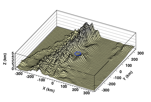
Figure 33: Topography in the vicinity of the Auger site. The surface array is centered at ${\rm X}={\rm Y}=0$. From Ref. [294].

To study the response of the detector, the outputs of PYTHIA and/or TAUOLA are used as input for the AIRES [295] air shower simulation package. The response of the surface detector array is simulated in detail using the Auger $\overline{\textrm{Off}}$ $\underline{\textrm{line}}$simulation package [296]. Atmospheric background muons are also simulated in order to study the impact on neutrino identification, as such accidental muons can be wrongly classified as shower particles. The background from hadronic showers above $10^{8}$ GeV is estimated to be ${\cal O}(1)$ in 20 years, so for the energy bin considered in this analysis, $9.5<\log_{10}(E_{\nu}/{\rm GeV})$, the background is negligible.

To establish benchmark neutrino rates, we use the Waxman-Bahcall bound [144] for the flux, $\Phi_{\rm WB}^{\nu_{\alpha}}=2.3\times 10^{-8}\,E_{\nu}^{-2}\leavevmode\nobreak\ {\rm GeV}^{-1}\,{\rm s}^{-1}\,{\rm cm}^{-2}\,{\rm sr}^{-1}$, and employ the acceptance computed by the simulations described above. In order to estimate the systematic uncertainty associated with our lack of knowledge of the dependence of the flux on energy, we consider several scenarios which plausibly bracket the range of possibilities:

1. $\Phi_{\rm WB}^{\nu_{\alpha}}(E_{\nu})=({\cal C}/E_{0})\,E_{\nu}^{-1}$,

2. $\Phi_{\rm WB}^{\nu_{\alpha}}(E_{\nu})={\cal C}\,E_{\nu}^{-2}$,

3. $\Phi_{\rm WB}^{\nu_{\alpha}}(E_{\nu})={\cal C}\,E_{0}\,E_{\nu}^{-3}$,

4. $\Phi_{\rm WB}^{\nu_{\alpha}}(E_{\nu})={\cal C}E_{\nu}^{-2}\,{\rm exp}[-\log_{10}(E_{\nu}/E_{0})^{2}/(2\sigma^{2})]$,

where ${\cal C}=2.3\times 10^{-8}$ ${\rm GeV}^{-1}\,{\rm s}^{-1}\,{\rm cm}^{-2}\,{\rm sr}^{-1}$, $E_{0}=10^{10}$ GeV, $\sigma=0.5$ GeV. The expected rates for the entire range over which Auger is sensitive are given in Table 6 and the rates for the high energy bin are given in Table 7.

Table 6: Expected events per year ($N_{i}$) at Auger in the energy range $8<\log_{10}(E_{\nu}/{\rm GeV})$, for various incident zenith angle ($\theta$) ranges, assuming the Waxman-Bahcall flux.

flux	up-going		down-going					ratio
	$\theta$	$N_{\nu_{\tau}}$	$\theta$	$N_{\nu_{e}}$	$N_{\nu_{\tau}}$	$N_{\nu_{\mu}}$	$N_{\nu_{\rm all}}$	$N_{\tau}/N_{\nu_{\rm all}}$
$(2)$	90-95	0.68	60-90	0.134	0.109	0.019	0.262	2.58
$(2)$	90-95	0.68	75-90	0.075	0.071	0.011	0.157	4.27

Table 7: Expected events per year ($N_{i}$) at Auger in the energy range $9.5<\log_{10}(E_{\nu}/{\rm GeV})<10.5$, for various incident zenith angle ($\theta$) ranges and the 4 flux models considered.

flux	up-going		down-going					ratio
	$\theta$	$N_{\nu_{\tau}}$	$\theta$	$N_{\nu_{e}}$	$N_{\nu_{\tau}}$	$N_{\nu_{\mu}}$	$N_{\nu_{\rm all}}$	$N_{\tau}/N_{\nu_{\rm all}}$
$(1)$	90-95	0.14	60-90	0.059	0.049	0.011	0.12	1.14
$(2)$	90-95	0.15	60-90	0.059	0.049	0.096	0.11	1.33
$(3)$	90-95	0.23	60-90	0.079	0.062	0.0123	0.15	1.53
$(4)$	90-95	0.12	60-90	0.046	0.037	0.0080	0.091	1.33
$(1)$	90-95	0.14	75-90	0.027	0.031	0.0056	0.064	2.14
$(2)$	90-95	0.15	75-90	0.026	0.029	0.0048	0.060	2.47
$(3)$	90-95	0.23	75-90	0.036	0.041	0.0062	0.083	2.75
$(4)$	90-95	0.12	75-90	0.021	0.024	0.0040	0.049	2.45

Table 8 contains a summary of systematic uncertainties on the ratio of the number of ES to QH events. The uncertainty in spectrum shape is taken from Table 7. The uncertainty on the parton structure of the nucleon is estimated by considering different PDFs (GRV92NLO [297] and CTEQ66c [298]). Finally, the uncertainty on the energy loss, $\beta_{\tau}$, of $\tau$ leptons as they propagate through the Earth’s crust is derived from [299, 300, 301, 302].

Table 8: Contributions to the systematic uncertainty on the Earth-skimming to quasi-horizontal event ratio. We have considered the energy range $9.5<\log_{10}(E_{\nu}/{\rm GeV})<10.5$ and the zenith angle range $75^{\circ}<\theta<90^{\circ}$.

ratio	flux	PDF	$\beta_{\tau}$	sum
	$+11\%$	$0\%$	$+24\%$	$\phantom{2.4666666}+26\%$
2.47				2.47
	$-13\%$	$-21\%$	$-25\%$	$\phantom{2.4666666}-35\%$

0.4.3 Auger discovery reach

Consider first a flux of Earth-skimming $\tau$ neutrinos with energy in the range $10^{9.5}\leavevmode\nobreak\ {\rm GeV}<E_{\nu}<10^{10.5}\leavevmode\nobreak\ {\rm GeV}$. The neutrinos can convert to $\tau$ leptons in the Earth via the charged current interaction $\nu_{\tau^{\pm}}N\rightarrow\tau^{\pm}X$. In the (perturbative) SM, the interaction path length for the neutrino is

$$L_{\rm CC}^{\nu}=\left[N_{A}\rho_{s}\sigma^{\nu}_{\rm CC}\right]^{-1}\ ,$$ (196)

where $\sigma^{\nu}_{\rm CC}$ is the charged current cross section for a neutrino energy $E_{\nu}=E_{0}$. The density of the material through which the neutrinos pass, $\rho_{s}$, is about $2.65\leavevmode\nobreak\ {\rm g}/{\rm cm}^{3}$ for the Earth’s crust. Here we have neglected neutral current interactions, which at these energies only reduce the neutrino energy by approximately 20%, which is within the systematic uncertainty. For $E_{0}\sim 10^{10}\leavevmode\nobreak\ {\rm GeV}$, $L_{\rm CC}^{\nu}\sim{\cal O}(100)$ km. Let us assume some hypothetical non-perturbative physics process enhances the $\nu N$ cross section. Then the interaction path length becomes

$$L_{\rm tot}^{\nu}=\left[N_{A}\rho_{s}(\sigma^{\nu}_{\rm CC}+\sigma^{\nu}_{\rm NP})\right]^{-1}\ ,$$ (197)

where $\sigma^{\nu}_{\rm NP}$ is the non-perturbative contribution to the cross section for $E_{\nu}=E_{0}$.

Once a $\tau$ is produced by a CC interaction, it can be absorbed in the Earth or escape and possibly decay, generating a detectable air shower. At these high energies, the $\tau$ propagation length in the Earth is dominated by energy loss rather than the finite $\tau$ lifetime. The energy loss can be expressed as

$$\frac{dE_{\tau}}{dz}=-(\alpha_{\tau}+\beta_{\tau}E_{\tau})\rho_{s}\ ,$$ (198)

where $\alpha_{\tau}$ characterizes energy loss due to ionization and $\beta_{\tau}$ characterizes losses through bremsstrahlung, pair production and hadronic interactions. At these energies, energy losses due to ionization turn out to be negligible, while $\beta_{\tau}\simeq 0.8\times 10^{-6}$ ${\rm cm}^{2}/{\rm g}$ [303]. From Eq. (198), we observe that the maximum path length for a detectable $\tau$ can be written

$$L^{\tau}=\frac{1}{\beta_{\tau}\rho_{s}}\ln\left(E_{\rm max}/E_{\rm min}\right)\ ,$$ (199)

where $E_{\rm max}\approx E_{0}$ is the energy at which the $\tau$ is created, and $E_{\rm min}$ is the minimal energy at which a $\tau$ can produce a shower big enough to be detected. For $E_{\rm max}/E_{\rm min}=10$, $L^{\tau}=11$ km.

The probability for a neutrino with incident nadir angle $\theta$ to emerge as a detectable $\tau$ is

$$P(\theta)=\int_{0}^{\ell}\frac{dz}{L_{\rm CC}^{\nu}}e^{-z/L_{\rm tot}^{\nu}}\ \Theta\left[z-(\ell-L^{\tau})\right],$$ (200)

where $\ell=2R_{\oplus}\cos\theta$ is the chord length of the intersection of the neutrino’s trajectory with the Earth, with $R_{\oplus}\approx 6371$ km the Earth’s radius. Note that we have neglected the possibility that non-perturbative processes could lead to a detectable signal, since the hadrons which dominate the final state will be absorbed in the Earth. The step function in Eq. (200) reflects the fact that a $\tau$ will only escape the Earth if $z+L^{\tau}>\ell$, as illustrated in Fig 34.

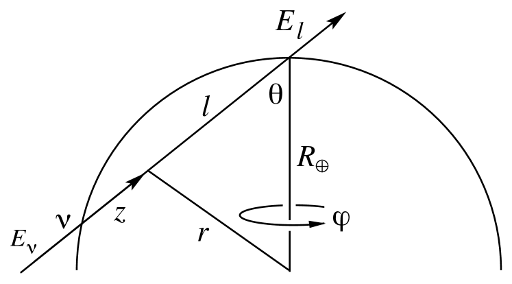
Figure 34: The chord length of the intersection of a neutrino with the Earth is $\ell=2R_{\oplus}\cos\theta$. In the figure, the neutrino produces a lepton $l$ after traveling some distance $z$ inside the Earth’s crust. If $z+L^{\tau}>\ell$, the lepton will escape the Earth and can generate an air shower. From Ref. [179].

Assuming an isotropic tau neutrino flux, the number of taus that emerge from the Earth with sufficient energy to be detected is proportional to an “effective solid angle”

$$\Omega_{\rm eff}\equiv\int P(\theta)\,\cos\theta\,d\cos\theta\,d\phi.$$ (201)

Evaluation of the integrals [286] yields the unfortunate expression

$$\Omega_{\rm eff}=2\pi\frac{L_{\rm tot}^{\nu}}{L_{\rm CC}^{\nu}}\left[e^{L^{\tau}/L_{\rm tot}^{\nu}}-1\right]\left[\left(\frac{L_{\rm tot}^{\nu}}{2R_{\oplus}}\right)^{2}-\left(\frac{L_{\rm tot}^{\nu}}{2R_{\oplus}}+\left(\frac{L_{\rm tot}^{\nu}}{2R_{\oplus}}\right)^{2}\right)e^{-2R_{\oplus}/L_{\rm tot}^{\nu}}\right]\ .$$ (202)

At the relevant energies, however, the neutrino interaction length satisfies $L_{\rm tot}^{\nu}\ll R_{\oplus}$. In addition, if the hypothesized non-perturbative cross section enhancement is less than typical hadronic cross sections, we have $L_{\rm tot}^{\nu}\gg L^{\tau}$. With these approximations, Eq. (202) simplifies to [287]

$$\Omega_{\rm eff}\approx 2\pi\frac{L_{\rm tot}^{\nu\,2}L^{\tau}}{4R_{\oplus}^{2}L_{\rm CC}^{\nu}}\ .$$ (203)

Equation (203) describes the functional dependence of the Earth-skimming event rate on the non-perturbative cross section. This rate is, of course, also proportional to the neutrino flux $\Phi^{\nu_{\rm all}}$ at $E_{0}$. Thus, the number of Earth-skimming neutrinos is given by

$$N_{\rm ES}\approx C_{\rm ES}\,\frac{\Phi^{\nu_{\rm all}}}{\Phi^{\nu_{\rm all}}_{0}}\frac{\sigma^{\nu\,2}_{\rm CC}}{\left(\sigma^{\nu}_{\rm CC}+\sigma^{\nu}_{\rm NP}\right)^{2}}\ ,$$ (204)

where $C_{\rm ES}$ is the number of Earth-skimming events expected for some benchmark flux $\Phi^{\nu_{\rm all}}_{0}$ in the absence of new physics.

In contrast to Eq. (204), the rate for quasi-horizontal showers has the form

$$N_{\rm QH}=C_{\rm QH}\frac{\Phi^{\nu_{\rm all}}}{\Phi^{\nu_{\rm all}}_{0}}\frac{\sigma^{\nu}_{\rm CC}+\sigma^{\nu}_{\rm NP}}{\sigma^{\nu}_{\rm CC}}\ ,$$ (205)

where $C_{\rm QH}$ is the number of quasi-horizontal events expected for flux $\Phi^{\nu_{\rm all}}_{0}$.

Now, without loss of generality, we normalize the neutrino flux to the Waxmann-Bahcall bound, i.e. $\Phi^{\nu_{\rm all}}_{0}\equiv\Phi^{\nu_{\rm all}}_{\rm WB}$. We use the expected rates for the the benchmark flux to determine the values of $C_{\rm ES}$ and $C_{\rm QH}$ in Eqs. (204) and (205), ($C_{\rm ES}=0.15$ and $C_{\rm QH}=0.06$, as shown in Table 7). Given a flux $\Phi^{\nu_{\rm all}}$ and new non-perturbative physics cross section $\sigma^{\nu}_{\rm NP}$, both $N_{\rm ES}$ and $N_{\rm QH}$ are determined. On the other hand, given just a quasi-horizontal event rate $N_{\rm QH}$, it is impossible to differentiate between an enhancement of the cross section due to non-perturbative physics and an increase of the flux. However, in the region where significant event rates are expected, the contours of $N_{\rm QH}$ and $N_{\rm ES}$, given by Eqs. (204) and (205), are more or less orthogonal and provide complementary information. This is illustrated in Fig. 35.

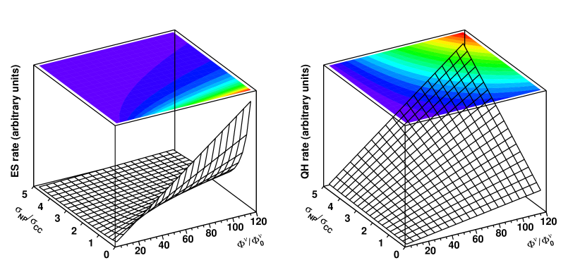
Figure 35: Event rates for Earth-skimming (left) and quasi-horizontal (right) events in the $\Phi^{\nu_{\rm all}}/\Phi_{0}^{\nu_{\rm all}}-\sigma_{\rm NP}/\sigma_{\rm CC}$ plane. Note that the contours are roughly orthogonal, and so the two types of event provide complementary information about flux and cross section.

With measurements of $N_{\rm QH}^{\rm obs}$ and $N_{\rm ES}^{\rm obs}$, both $\sigma^{\nu}_{\rm NP}$ and $\Phi^{\nu_{\rm all}}$ may be determined independently, and neutrino interactions beyond the (perturbative) SM may be unambiguously identified.

Figure 36: Projected determination of neutrino fluxes and cross sections at $\sqrt{s}\approx 250$ TeV from future Auger data. The different shaded regions indicate the 90%, 95%, 99% and 3$\sigma$ confidence level contours in the $\Phi^{\nu_{\rm all}}/\Phi_{0}^{\nu_{\rm all}}-\sigma_{\rm NP}/\sigma_{\rm CC}$ plane, for $N^{\rm obs}_{\rm ES}=1$, $N^{\rm obs}_{\rm QH}=10$ (left), $N^{\rm obs}_{\rm ES}=1$, $N^{\rm obs}_{\rm QH}=7$ (middle), and $N^{\rm obs}_{\rm ES}=1$, $N^{\rm obs}_{\rm QH}=5$ (right). The dashed line indicates the result of including the systematic uncertainty on the NLO QCD CC neutrino-nucleon cross section. From Ref. [294].

We now turn to determining the projected sensitivity of Auger to neutrino fluxes and cross sections. The quantities $N_{\rm ES}$ and $N_{\rm QH}$ as defined in Eqs. (204) and (205) can be regarded as the theoretical values of these events, corresponding to different points in the $\Phi^{\nu_{\rm all}}/\Phi_{0}^{\nu_{\rm all}}-\sigma_{\rm NP}/\sigma_{\rm CC}$ parameter space. For a given set of observed rates $N^{\rm obs}_{\rm ES}$ and $N^{\rm obs}_{\rm QH}$, two curves are obtained in the two-dimensional parameter space by setting $N^{\rm obs}_{\rm ES}=N_{\rm ES}$ and $N^{\rm obs}_{\rm QH}=N_{\rm QH}$. These curves intersect at a point, yielding the most probable values of flux and cross section for the given observations. Fluctuations about this point define contours of constant $\chi^{2}$ in an approximation to a multi-Poisson likelihood analysis [304]. The contours are defined by

$$\chi^{2}=\sum_{i}2\,\left[N_{i}-N_{i}^{\rm obs}\right]+2\,N_{i}^{\rm obs}\,\ln\left[N_{i}^{\rm obs}/N_{i}\right]\,\,,$$ (206)

where $i=$ ES, QH [305]. In Fig. 36, we show results for three representative cases. Assuming ($N^{\rm obs}_{\rm ES}=1$, $N^{\rm obs}_{\rm QH}=10$), ($N^{\rm obs}_{\rm ES}=1$, $N^{\rm obs}_{\rm QH}=7$), and ($N^{\rm obs}_{\rm ES}=1$, $N^{\rm obs}_{\rm QH}=5$) we show the 90%, 95%, 99% and 3$\sigma$ CL contours for 2 d.o.f. ($\chi^{2}=4.61,\ 5.99,\ 9.21,$ and 11.83, respectively). For $N^{\rm obs}_{\rm ES}=1$ and $N^{\rm obs}_{\rm QH}=10$, the possibility of a SM interpretation along the $\sigma^{\nu}_{\rm NP}=0$ axis (taking into account systematic uncertainties) would be excluded at greater than 99% CL for any assumed flux.

In summary, we have found that observation of 1 Earth-skimming and 10 quasi-horizontal events would exclude the (perturbative) SM at the 99% CL. Thus the expected low neutrino “luminosity” is not at all a show-stopper, and the observatory has the potential to uncover new physics at scales exceeding those accessible to the LHC. If new non-perturbative physics exists, a decade or so would be required to uncover it at Auger in the best case scenario (cosmic neutrino flux at the Waxman-Bahcall level and $\nu N$ cross section about an order of magnitude above the SM prediction). Of course future CR experiments should benefit from a much larger aperture, making such discovery conceivable in a short time scale. An optimist may even imagine the possibility of probing QCD dynamics [306].

.5 Cosmogenic $\bm{\beta}$-DK and $\bm{A^{*}}$ processes

If UHECRs are heavy nuclei, the relic photons can excite the GDR at nucleus energies $E\mathrel{\hbox to0.0pt{\lower 4.0pt\hbox{\hskip 1.0pt$\sim$}\hss}\raise 1.0pt\hbox{$>$}}10^{11}$ GeV (corresponding to $\omega_{r}^{\rm GDR}\sim 10\leavevmode\nobreak\ {\rm MeV}-30\leavevmode\nobreak\ {\rm MeV}$ in the nuclear rest frame), and thus there should be accompanying photo-dissociated free neutrons, themselves a source of $\beta$-decay antineutrinos. The decay mean free path of a neutron is $c\Gamma_{n}\overline{\tau}_{n}=(E_{n}/10^{11}$ GeV) Mpc, the lifetime being boosted from its rest frame value $\overline{\tau}_{n}=886$ s to its lab value via $\Gamma_{n}=E_{n}/m_{n}$. Compared to cosmic distances $\mathrel{\hbox to0.0pt{\lower 4.0pt\hbox{\hskip 1.0pt$\sim$}\hss}\raise 1.0pt\hbox{$>$}}100$ Mpc, the decay of even the boosted neutron may be taken as nearly instantaneous, and thus all free neutrons are themselves a source of $\beta$-decay cosmogenic antineutrinos. The neutron emissivity ${\cal Q}_{n}(E_{n}),$ defined as the mean number of neutrons emitted per comoving volume per unit time per unit energy as measured at the source can be estimated as follows. Neutrons with energies above $10^{9.3}$ GeV have parent iron nuclei with $\Gamma>\Gamma_{0}\approx 2\times 10^{9}$ which are almost completely disintegrated in distances of less than 100 Mpc (see Sec. 0.2.3). Thus, it is reasonable to define a characteristic time $\tau_{{}_{\Gamma}}$ given by the moment at which the number of nucleons is reduced to $1/e$ of its initial value $A$, and presume the nucleus, emitted at distance $d$ from the Earth, is a traveling source that at $D\approx(d-c\tau_{{}_{\Gamma}})$ disintegrates into $A$ nucleons all at once [120]. Then, the number of neutrons with energy $E_{n}=E_{A}/A$ can be approximated by the product of 1/2 the number of nucleons generated per nucleus and the number of nuclei emitted, i.e. ${\cal Q}_{n}(E_{n})=$N${\cal Q}_{A}$, where $N=A-Z$ is the mean neutron number of the source nucleus. Now, to obtain an estimate of the diffuse antineutrino flux one needs to integrate over the population of nucleus-emitting-sources out to the horizon [307, 308]

$$\Phi_{\overline{\nu}_{e}} = \frac{1}{4\pi\,H_{0}}\,\int dE_{n}\,{\cal Q}_{n}(E_{n})\,\,\left[1-\exp\left(-\frac{D\,m_{n}}{E_{n}\,\overline{\tau}_{n}}\right)\right]\,\,\int_{0}^{Q}d\epsilon_{\overline{\nu}}\,\frac{dP}{d\epsilon_{\overline{\nu}}}(\epsilon_{\overline{\nu}})$$ (207)

$$\times\int_{-1}^{1}\frac{d\cos\overline{\theta}_{\overline{\nu}}}{2}\;\delta\left[E_{\overline{\nu}}-E_{n}\,\epsilon_{\overline{\nu}}\,(1+\cos\overline{\theta}_{\overline{\nu}})/m_{n}\right]\,,$$

where the $r^{2}$ in the volume integral is compensated by the usual $1/r^{2}$ fall-off of flux per source. Here, $H_{0}$ is the Hubble constant, $E_{\overline{\nu}}$ and $E_{n}$ are the antineutrino and neutron energies in the lab, $\overline{\theta}_{\overline{\nu}}$ is the antineutrino angle with respect to the direction of the neutron momentum in the neutron rest-frame, and $\epsilon_{\overline{\nu}}$ is the antineutrino energy in the neutron rest-frame. The last three variables are not observed by a laboratory neutrino-detector, and so are integrated over. The observable $E_{\overline{\nu}}$ is held fixed. The delta-function relates the neutrino energy in the lab to the three integration variables. The parameters appearing in Eq. (207) are the neutron mass and rest-frame lifetime ($m_{n}$ and $\overline{\tau}_{n}$). Finally, $dP/d\epsilon_{\overline{\nu}}$ is the normalized probability that the decaying neutron produces a $\overline{\nu}$ with energy $\epsilon_{\overline{\nu}}$ in the neutron rest-frame. Note that the maximum $\overline{\nu}$ energy in the neutron rest frame is very nearly $Q\equiv m_{n}-m_{p}-m_{e}=0.71$ MeV. Integration of Eq. (207) can be easily accomplished, especially when two good approximations are applied [309] . The first approximation is to think of the $\beta$–decay as a $1\to 2$ process of $\delta m_{N}\to e^{-}+\overline{\nu},$ in which the neutrino is produced monoenergetically in the rest frame, with $\epsilon_{\overline{\nu}}=\epsilon_{0}\simeq\delta m_{N}(1-m_{e}^{2}/\delta^{2}m_{N})/2\simeq 0.55$ MeV, where $\delta m_{N}\simeq 1.30$ MeV is the neutron-proton mass difference. In the lab, the ratio of the maximum $\overline{\nu}$ energy to the neutron energy is $2\epsilon_{0}/m_{n}\sim 10^{-3},$ and so the boosted $\overline{\nu}$ has a spectrum with $E_{\overline{\nu}}\in(0,10^{-3}\,E_{n}).$ The second approximation is to replace the neutron decay probability $1-e^{-Dm_{n}/E_{n}\overline{\tau}_{n}}$ with a step function $\Theta(E_{n}^{\rm max}-E_{n})$ at some energy $E_{n}^{\rm max}\sim{\cal O}(D\,m_{n}/\overline{\tau}_{n})=(D/10\leavevmode\nobreak\ {\rm Mpc})\times 10^{12}$ GeV. Combining these two approximations we obtain

$$\Phi_{\overline{\nu}_{e}}=\frac{m_{n}}{8\,\pi\,\epsilon_{0}\,H_{0}}\int_{E_{A}^{\rm min}}^{E_{A}^{\rm max}}\frac{dE_{A}}{E_{A}/A}\,\,{\cal Q}_{A}(E_{A})\,\,,$$ (208)

where $E_{A}^{\rm min}\equiv{\rm max}\{E_{A,\Gamma_{0}},\frac{A\,m_{n}E_{\overline{\nu}}}{2\epsilon_{0}}\},$ and $E_{A}^{\rm max}$ is the energy cutoff at the nucleus-emitting-source $\ll A(D/10\leavevmode\nobreak\ {\rm Mpc})\times 10^{12}$ GeV. For ${\cal Q}_{A}\propto E_{A}^{-\alpha},$ integration of Eq. (208) leads to

$$\Phi_{\overline{\nu}_{e}}(E_{\overline{\nu}})\approx 10^{6}\left(\frac{E_{A,\Gamma_{0}}}{E_{A}^{\rm max}}\right)^{\alpha}\left[\left(\frac{E^{\rm max}_{\overline{\nu}}}{E_{\overline{\nu}}}\right)^{\alpha}-1\right]\,\left.{\cal Q}_{A}\right|_{\Gamma_{0}}\,\,,$$ (209)

where $E_{\overline{\nu}}\mathrel{\hbox to0.0pt{\lower 4.0pt\hbox{\hskip 1.0pt$\sim$}\hss}\raise 1.0pt\hbox{$>$}}10^{6.3}\,(56/A)$ GeV and

$$E_{\overline{\nu}}^{\rm max}=\frac{2\epsilon_{0}}{m_{n}}\,\,\frac{E_{A}^{\rm max}}{A}\sim 10^{7.3}\,\,\left(\frac{56}{A}\right)\,\,\left(\frac{E_{A}^{\rm max}}{10^{12}\leavevmode\nobreak\ {\rm GeV}}\right)\,\,{\rm GeV}\,.$$ (210)

The sub-PeV antineutrino spectrum is flat, as all the free neutrons have sufficient energy $E_{n}\mathrel{\hbox to0.0pt{\lower 4.0pt\hbox{\hskip 1.0pt$\sim$}\hss}\raise 1.0pt\hbox{$>$}}E_{\Gamma_{0}}/A,$ to contribute equally to all the $\overline{\nu}$ energy bins below $10^{6}$ GeV. Taking $\alpha=2$ as a reasonable example, and inputting the observational value for iron nuclei, $\left.E^{2}_{A,\Gamma_{0}}\,\ J_{\rm CR}\right|_{\Gamma_{0}}\approx 10^{5}$ eV m^-2 s^-1 sr^-1, Eq. (209) becomes

$$E_{\overline{\nu}}^{2}\ \Phi_{\overline{\nu}_{e}}\approx 4\times 10^{1}\,\,\left(\frac{56}{A}\right)\,\,{\rm eV}\,{\rm m}^{-2}\,\,{\rm s}^{-1}\,\,{\rm sr}^{-1}\,.$$ (211)

Note that the $\beta$-decay process gives initial antineutrino flavor ratios $1:0:0$ and Earthly ratios nearly $3:1:1.$ Compared to full-blown Monte Carlo simulations [310, 311], this back of the envelope calculation underestimates the flux by about 30%. This is because the preceeding calculation does not account for possible neutrons produced in $p\gamma_{\rm CMB}$ collisions. Of course the situation described above represents the most extreme case, in which all cosmic rays at the end of the spectrum are heavy nuclei. A more realistic guess would be that the composition at the end of the spectrum is mixed.

Photodisintegration of high energy nuclei is followed by immediate photo-emission from the excited daughter nuclei. For brevity, we label the photonuclear process $A+\gamma\to A^{\prime*}+X$, followed by $A^{\prime*}\to A^{\prime}+\gamma$-ray as “$A^{*}$” [312]. The GDR decays dominantly by the statistical emission of a single nucleon, leaving an excited daughter nucleus $(A-1)^{*}$. The excited daughter nuclei typically de-excite by emitting one or more photons of energies $\epsilon_{\gamma}^{\rm dxn}\sim 1-5$ MeV in the nuclear rest frame. The lab-frame energy of the $\gamma$-ray is then $\epsilon_{\gamma}^{\rm LAB}=\Gamma_{A}\,\epsilon_{\gamma}^{\rm dxn}$, where $\Gamma_{A}=E_{A}/m_{A}$ is the boost factor of the nucleus in the lab.

Of interest here is the $\gamma$-ray flux produced when the photo-dissociated nuclear fragments produced on the CMB and CIB de-excite. These $\gamma$-rays create chains of electromagnetic cascades on the CMB and CIB, resulting in a transfer of the initial energy into the so-called Fermi-LAT region, which is bounded by observation to not exceed $\omega_{\rm cas}\sim 5.8\times 10^{-7}{\rm eV/cm^{3}}$ [170]. Fortunately, we can finesse the details of the calculation by arguing in analogy to work already done. The photodisintegration chain produces one $\beta$-decay neutrino with energy of order 0.5 MeV in the nuclear rest frame, for each neutron produced. Multiplying this result by 2 to include photodisintegration to protons in addition to neutrons correctly weights the number of steps in the chain. Each step produces on average one photon with energy $\sim 3$ MeV in the nuclear rest frame. In comparison, about 12 times more energy is deposited into photons. Including the factor of 12 relating $\omega_{\gamma}$ to $\omega_{\bar{\nu}_{e}}$, we find from (211) that cosmogenic photodisintegration/de-excitation energy, $\omega_{\rm cas}\sim 1.4\times 10^{-11}\,(56/A)$ eV/cm³, is more than three orders of magnitude below the Fermi-LAT bound. This result appears to be nearly invariant with respect to varying the maximum energy of the Fe injection spectrum (with a larger $E_{\rm max}$, the additional energy goes into cosmogenic pion production). Thus, there is no constraint on a heavy nuclei cosmic-ray flux from the $A^{*}$ mechanism.

Neutron emission from a cosmological distribution of CR sources would also lead to a flux of $\overline{\nu}_{e}$. In analogy to our previous estimate, we sum over the neutron-emitting sources out to the edge of the universe; Eq. (208) becomes [314]

$$\Phi_{\overline{\nu}_{e}}=\frac{m_{n}}{8\,\pi\,\epsilon_{0}\,H_{0}}\int_{\frac{m_{n}E_{\overline{\nu}}}{2\epsilon_{0}}}^{E_{n}^{\rm max}}\frac{dE_{n}}{E_{n}}\,\,{\cal Q}_{n}(E_{n})\,\,,$$ (212)

where ${\cal Q}_{n}(E_{n})$ is the neutron volume emissivity. An upper limit can be placed on ${\cal Q}_{n}$ by assuming an extreme situation in which all the CRs escaping the source are neutrons, i.e., $\dot{\epsilon}_{{}_{\rm CR}}^{[10^{10},10^{12}]}=\int dE_{n}\,\,E_{n}\,\,{\cal Q}_{n}(E_{n}).$ With the production rate of ultrahigh energy protons (91), and an assumed injection spectrum ${\cal Q}_{n}\propto E_{n}^{-2},$ Eq. (212) gives

$$E_{\nu}^{2}\ \Phi_{\overline{\nu}_{e}}\approx 3\times 10^{-11}\,\,{\rm GeV}\,{\rm cm}^{-2}\,{\rm s}^{-1}\,{\rm sr}^{-1}\,\,,$$ (213)

which is about three orders of magnitude below the Waxman-Bahcall bound.

.6 Energy density of the EM cascade

EM interactions of photons and leptons with the extragalactic radiation backgrounds and magnetic field can happen on time-scales much shorter than their production rates. The relevant processes with background photons contributing to the differential interaction rates $\gamma_{ee}$, $\gamma_{\gamma e}$, and $\gamma_{e\gamma}$ are inverse Compton scattering (ICS), $e^{\pm}+\gamma_{\rm bgr}\to e^{\pm}+\gamma$, pair production (PP), $\gamma+\gamma_{\rm bgr}\to e^{+}+e^{-}$, double pair production (DPP) $\gamma+\gamma_{\rm bgr}\to e^{+}+e^{-}+e^{+}+e^{-}$, and triple pair production (TPP), $e^{\pm}+\gamma_{\rm bgr}\to e^{\pm}+e^{+}+e^{-}$ [106, 315].

High energetic electrons and positrons may also lose energy via synchrotron radiation in the intergalactic magnetic field $B$ with a random orientation $\sin\theta$ with respect to the velocity vector. We will assume in the following that the field strength $B=10^{-12}$ G. This leads to an efficient transfer of energy into the EM cascade. The synchrotron power spectrum (W eV^-1) has the form

$$\mathcal{P}(E_{e},E_{\gamma})=\frac{\sqrt{3}\alpha}{2\pi}\frac{eB\sin\theta}{m_{e}}F(E_{\gamma}/E_{\rm c})\,;\qquad F(t)\equiv t\int_{t}^{\infty}dz\,K_{5/3}(z)\,,$$ (214)

where $K_{5/3}$ is the modified Bessel function and $E_{\rm c}=(3eB\sin\theta/2m_{e})(E_{e}/m_{e})^{2}$. This can be treated as a continuous energy loss of the electrons and positrons with a parameter

$$b_{\rm syn}(E_{e})=\frac{1}{2}\int d\cos\theta\int dE_{\gamma}\mathcal{P}(E_{e},E_{\gamma})=\frac{4\alpha}{9}\left(\frac{eB}{m_{e}}\right)^{2}\left(\frac{E_{e}}{m_{e}}\right)^{2}\,.$$ (215)

We will assume in the calculation that the intergalactic magnetic field is primordial with a (flux-conserving) redshift dependence $B(z)=(1+z)^{2}B(0)$. Note that the synchrotron energy loss has then a redshift dependence similar to BH pair production in the CMB, i.e. $b_{\rm syn}(z,E)=(1+z)^{2}b_{\rm syn}(0,(1+z)E)$. It is also convenient to define $\gamma_{e\gamma}^{\rm syn}(E_{e},E_{\gamma})\equiv\mathcal{P}(E_{e},E_{\gamma})/E_{\gamma}$, which has an analogous redshift dependence, i.e. $\gamma_{e\gamma}^{\rm syn}(z,E_{e},E_{\gamma})=(1+z)^{4}\gamma_{e\gamma}^{\rm syn}(0,(1+z)E_{e},(1+z)E_{\gamma})$.

The fast evolution of the cascade is governed by the set of differential equations,

$$\partial_{\hat{t}}Y_{e}(E)= -\Gamma_{e}(E)Y_{e}(E)+\partial_{E}(b(E)Y_{e}(E))+\int dE^{\prime}\left[\gamma_{\gamma e}(E^{\prime},E)Y_{\gamma}(E^{\prime})+\gamma_{ee}(E^{\prime},E)Y_{e}(E^{\prime})\right]\,,$$

$$\partial_{\hat{t}}Y_{\gamma}(E)= -\Gamma_{\gamma}(E)Y_{\gamma}(E)+\int dE^{\prime}\frac{\mathcal{P}(E^{\prime},E)}{E}Y_{e}(E^{\prime})+\int dE^{\prime}\gamma_{e\gamma}(E^{\prime},E)Y_{e}(E^{\prime})\,,$$ (216)

which determines the evolution on short time-scales $\Delta\hat{t}\,\Gamma_{p\gamma}\ll 1$ (the redshift $z$ is kept fixed meanwhile). The initial condition $Y_{\gamma/e}(E)|_{\hat{t}=0}$ is given by the sum of previously developed cascades and the newly generated contributions from proton interactions.

The solution of the system (216) for an infinitesimally small step $\Delta\hat{t}$ can be written for a discrete energy spectrum, $N_{i}\simeq\Delta E_{i}Y_{i}$, as

$$\begin{pmatrix}N_{\gamma}\\ N_{e}\end{pmatrix}_{i}(\hat{t}+\Delta\hat{t})\simeq\sum_{j}\begin{pmatrix}T_{\gamma\gamma}(\Delta\hat{t})&T_{e\gamma}(\Delta\hat{t})\\ T_{\gamma e}(\Delta\hat{t})&T_{ee}(\Delta\hat{t})\end{pmatrix}_{ji}\begin{pmatrix}N_{\gamma}\\ N_{e}\end{pmatrix}_{j}(\hat{t})\,.$$ (217)

With the transition matrix $\mathcal{T}(\Delta\hat{t})$, defined by Eq. (217), we can efficiently follow the development of the EM cascade over a distance $\Delta t=2^{N}\Delta\hat{t}$ via matrix doubling [167]:

$$\mathcal{T}(2^{N}\Delta\hat{t})\simeq\left[\mathcal{T}(\Delta\hat{t})\right]^{2N}\,.$$ (218)

The total energy of the cascade can be obtained by integrating Eq. (120):

$$\frac{d}{dt}\left[\int dE\ E{\mathscr{Z}}_{\rm cas}(z,E)\right]=-\int dEE\partial_{\mathscr{E}}\left[b_{\rm cas}(z,\mathscr{E})\mathscr{Z}_{\rm p}(z,E)\right]\,.$$ (219)

Integrating the r.h.s. by parts yields

$${\rm r.h.s.}=-\int dE\partial_{E}\left[E\frac{1}{1+z}b_{\rm cas}(z,\mathscr{E}){\mathscr{Z}}_{p}(z,E)\right]+\int dE\frac{1}{1+z}b_{\rm cas}(z,\mathscr{E})\mathscr{Z}_{p}(z,E)\,.$$ (220)

The first term vanishes since $b_{\rm cas}=0$ for sufficiently low energies and $\mathscr{Z}_{p}=0$ beyond the maximal energy. The time integration of the l.h.s. between the present epoch ($t=0$) and the first sources ($t_{\rm max}$) gives

$$\int_{0}^{t_{\rm max}}dt[{\rm l.h.s.}]=\int dEEn_{\rm cas}(E)=\omega_{\rm cas}\,,$$ (221)

hence we obtain Eq. (121).

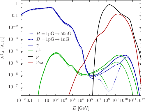
Figure 37: Cosmogenic photon (blue lines) and neutrino (red line) fluxes from a "vanilla" proton test-spectrum (shown as black line) of UHECRs, assuming two exponential cutoffs ($E_{\rm min}=10^{8}\leavevmode\nobreak\ {\rm GeV}$ and $E_{\rm max}=10^{11.5}\leavevmode\nobreak\ {\rm GeV}$), power index $\gamma=2$ and evolution with $n=3$ and $0<z<2$. The fluxes are computed for 3 extragalactic magnetic field strengths: 1 pG, 1 nG, and 50 nG. Proton diffusion in extragalactic magnetic fields $B>>{\rm nG}$ has not yet been included in the calculation. We have neglected radiative losses of muons and pions before decaying into neutrinos; the energy loss in muons is down by a factor $10^{6}$ compared to electrons. This figure is courtesy of Markus Ahlers.

Synchrotron radiation in strong magnetic fields, $1\leavevmode\nobreak\ {\rm nG}\lesssim B\lesssim 50\leavevmode\nobreak\ {\rm nG}$, can also by-pass the EM cascade and transfer energy to sub-GeV photons that are unconstrained by the Fermi-LAT spectrum [318]. This would be relevant for electrons around $E_{e}\sim 10^{9}$ GeV, where synchrotron loss starts to dominate over ICS loss in the CMB; see Fig. 37. From Eqs. (20) and (27) we can verify that $\langle E_{\gamma}^{\rm syn}\rangle\lesssim 1\leavevmode\nobreak\ {\rm GeV}$. Of course, reaching a 50 nG field requires some astrophysical generator to augment the primordial field. For simplicity, we have taken the redshift evolution of the generator to be the same as the evolution of the primordial field. If were to assume an evolution which follows SFR, this will not significantly alter our conclusions.

.7 TOTal Elastic and diffractive cross section Measurement

The TOTEM experiment is dedicated to the measurement of the total $pp$ cross section with the luminosity independent method based on the Optical Theorem,

$$\sigma_{\rm tot}={8\pi\over\sqrt{s}}\;{\rm Im}f(0)\,\,,$$ (222)

where $f(\vartheta)$ satisfies

$${d\sigma_{\rm el}\over dt}={4\pi\over s}\;{d\sigma_{\rm el}\over d\Omega}={4\pi\over s}\;|f(\vartheta)|^{2}\,\,,$$ (223)

with $\vartheta$ the angle of the scattered proton with respect to the beam direction. Squaring Eq. (222) we obtain

$$\sigma^{2}_{\rm tot}={16\pi\,\,{\rm Im}^{2}f(0)\over{\rm Re}^{2}f(0)+{\rm Im}^{2}f(0)}\;\left.{d\sigma_{\rm el}\over dt}\right|_{t=0}={16\pi\over 1+\rho^{2}}\;\;\frac{[dN_{\rm el}/dt]_{t=0}}{{\cal L}}\,,$$ (224)

where ${\cal L}$ is the integrated luminosity. Now, following [321, 322], we can obtain the total cross section independently from ${\cal L}$, by using $\sigma_{\rm tot}=(\sigma_{\rm el}+\sigma_{\rm inel})=(N_{\rm el}+N_{\rm inel})/{\cal L},$

$$\sigma_{\rm tot}={16\pi\over 1+\rho^{2}}\,{[dN_{\rm el}/dt]_{t=0}\over(N_{\rm el}+N_{\rm inel})}\,.$$ (225)

Here, $N_{\rm el}$ and $N_{\rm inel}$ are the numbers of elastic and inelastic events, and $\rho=0.10\pm 0.01$ is the ratio between the real and imaginary parts of the forward scattering amplitude [323]. The difficult aspect of this measurement is obtaining a good extrapolation of the cross section for low momentum transfer. Recall that $-t=s\,(1-\cos\vartheta)/2\simeq s\,\vartheta^{2}/4$, and so $t\to 0$ implies a measurement in the extreme forward direction. The TOTEM experiment aims to measure down to values of $|t|\approx\times 10^{-3}\leavevmode\nobreak\ \rm{GeV}^{2},$ which corresponds to $\vartheta\approx 4.5\leavevmode\nobreak\ \mu$rad [324].

.8 Raiders of the lost holy grail

In 1976 ’t Hooft observed that the Standard Model does not strictly conserve baryon and lepton number [325, 326]. Rather, non-trivial fluctuations in $SU(2)$ gauge fields generate an energy barrier interpolating between topologically distinct vacua. An index theorem describing the fermion level crossings in the presence of these fluctuations reveals that neither baryon nor lepton number is conserved during the transition, but only the combination $B-L.$ Inclusion of the Higgs field in the calculation modifies the original instanton configuration [327]. An important aspect of this modification (called the “sphaleron”) is that it provides an explicit energy scale of about 10 TeV for the height of the barrier. This barrier can be overcome through thermal transitions at high temperatures [328, 329, 330], providing an important input to any calculation of cosmological baryogenesis. More speculatively, it has been suggested [331, 332, 333] that the topological transition could take place in two particle collisions at very high energy. The anomalous electroweak contribution to the partonic process can be written as

$$\hat{\sigma}_{i}(\hat{s})=5.3\times 10^{3}{\rm mb}\cdot e^{-(4\pi/\alpha_{W})\ F_{W}(\epsilon)}\ \ ,$$ (226)

where $\alpha_{W}\simeq 1/30$, the tunneling suppression exponent $F_{W}(\epsilon)$ is sometimes called the “holy-grail function”, and $\epsilon\equiv\sqrt{\hat{s}}/(4\pi m_{W}/\alpha_{W})\simeq\sqrt{\hat{s}}/30$ TeV. Thus, it is even possible that at or above the sphaleron energy the cross-section could be of ${\cal O}(\rm mb)$ [334]. Of particular interest here would be an enhancement of the neutrino cross section over the perturbative SM estimates, say by an order of magnitude in the energy range $9.5<\log_{10}(E_{\nu}/{\rm GeV})<10.5$.

The argument for strong damping of the anomalous cross section for $\sqrt{\hat{s}}\gtrsim$ 30 TeV was convincingly demonstrated in [335, 336], in the case that the classical field providing the saddle point interpolation between initial and final scattering states is dominated by spherically symmetric configurations. This $O(3)$ symmetry allows the non-vacuum boundary conditions to be fully included in extremizing the effective action. In [337] it was shown that a sufficient condition for the $O(3)$ dominance is that the interpolating field takes the form of a chain of “lumps” which are well-separated, so that the each lump lies well into the exponentially damped region of its nearest neighbors. However, we are not aware of any reason that such lumped interpolating fields should dominate the effective action. It is thus of interest to explore the other extreme, in which non-spherically symmetric contributions dominate the effective action (and let experiment be the arbiter).

It was shown [334] that for the simple sphaleron configuration $s$-wave unitarity is violated for $\sqrt{\hat{s}}>4\pi M_{W}/\alpha_{W}\sim 36$ TeV. If for $\sqrt{\hat{s}}>36$ TeV we saturate unitarity in each partial wave, then this yields a geometric parton cross section $\pi R^{2}$, where $R$ is some average size of the classical configuration. As a fiducial value we take the core size of the Manton-Klinkhamer sphaleron, $R\simeq 4/M_{W}\simeq 10^{-15}$ cm. In this simplistic model, the $\nu N$ cross section is

$$\sigma^{\nu N}_{\rm black\,disk}(E_{\nu})=\pi R^{2}\ \int_{x_{\rm min}}^{1}\sum_{\rm partons}f(x)\ dx\,,$$ (227)

where $x_{\rm min}=\hat{s}_{\rm min}/s=(36)^{2}/2ME_{\nu}\simeq 0.065$. In the region $0.065<x<3(0.065)$ the PDF for the up and down quarks is well approximated by $f\simeq 0.5/x$, so the expression for the cross section becomes

$$\sigma^{\nu N}_{\rm black\,disk}(E_{\nu}) \simeq \pi R^{2}\,\,(0.5)\,\,(\ln 3)\,\,(2/2)$$ (228)

$$\simeq 1.5\times 10^{-30}{\rm cm}^{2}\,,$$

where the last factor of 2/2 takes into account the (mostly) 2 contributing quarks $(u,d)$ in this range of $x,$ and the condition that only the left-handed ones contribute to the scattering. This is about 80 times the SM cross section. Of course this calculation is very approximate and the cross section can easily be smaller by a factor of 10 (e.g. if $R$ is 1/3 of the fiducial value used).

References

- [1] V. F. Hess, Phys. Z. 13, 1804 (1912).
- [2] P. Auger, R. Maze, T. Grivet-Meyer, Comptes Rendus 206, 1721 (1938).
- [3] P. Auger, P. Ehrenfest, R. Maze, J. Daudin, Robley, and A. Fréon, Rev. Mod. Phys. 11, 288 (1939).
- [4] M. Nagano and A. A. Watson, Rev. Mod. Phys. 72, 689 (2000).
- [5] A. Letessier-Selvon and T. Stanev, arXiv:1103.0031 [astro-ph.HE].
- [6] L. Anchordoqui, T. C. Paul, S. Reucroft and J. Swain, Int. J. Mod. Phys. A 18, 2229 (2003) [arXiv:hep-ph/0206072].
- [7] T. Abu-Zayyad et al., Nucl. Instrum. Meth. A 450, 253 (2000).
- [8] R. M. Baltrusaitis et al., Nucl. Instrum. Meth. A 240, 410 (1985).
- [9] J. Abraham et al. [Pierre Auger Collaboration], Nucl. Instrum. Meth. A 523, 50 (2004).
- [10] J. Abraham et al. [Pierre Auger Collaboration], Nucl. Instrum. Meth. A 613, 29 (2010).
- [11] J. A. Abraham et al. [Pierre Auger Collaboration], Nucl. Instrum. Meth. A 620, 227 (2010) [arXiv:0907.4282].
- [12] P. Abreu et al. [Pierre Auger Collaboration], Astropart. Phys. 34, 368 (2011) [arXiv:1010.6162 [astro-ph.HE]].
- [13] Y. Takahashi et al. [JEM-EUSO Collaboration], New J. Phys. 11, 065009 (2009) [arXiv:0910.4187 [astro-ph.HE]].
- [14] T. Weiler, private communication.
- [15] C. Amsler et al. [Particle Data Group], Phys. Lett. B 667, 1 (2008).
- [16] M. Aglietta et al. [EAS-TOP Collaboration], Astropart. Phys. 21, 583 (2004).
- [17] T. Antoni et al. [KASCADE Collaboration], Astropart. Phys. 24, 1 (2005) [arXiv:astro-ph/0505413].
- [18] W. D. Apel et al [KASCADE Collaboration], Astropart. Phys. 31, 86 (2009) [arXiv:0812.0322 [astro-ph]].
- [19] J. Bluemer, R. Engel and J. R. Hoerandel, Prog. Part. Nucl. Phys. 63, 293 (2009) [arXiv:0904.0725 [astro-ph.HE]].
- [20] M. Hillas, Phys. Lett. A 24, 677 (1967).
- [21] V. Berezinsky, A. Z. Gazizov and S. I. Grigorieva, Phys. Rev. D 74, 043005 (2006) [arXiv:hep-ph/0204357].
- [22] R. Aloisio, V. Berezinsky, P. Blasi, A. Gazizov, S. Grigorieva and B. Hnatyk, Astropart. Phys. 27, 76 (2007) [arXiv:astro-ph/0608219].
- [23] G. Cocconi, Astropart. Phys. 4, 281 (1996).
- [24] A. A. Penzias and R. W. Wilson, Astrophys. J. 142, 419 (1965).
- [25] K. Greisen, Phys. Rev. Lett. 16, 748 (1966).
- [26] G. T. Zatsepin and V. A. Kuzmin, JETP Lett. 4, 78 (1966) [Pisma Zh. Eksp. Teor. Fiz. 4, 114 (1966)].
- [27] J. N. Bahcall and E. Waxman, Phys. Lett. B 556, 1 (2003) [arXiv:hep-ph/0206217].
- [28] R. U. Abbasi et al. [HiRes Collaboration], Phys. Rev. Lett. 100, 101101 (2008) [arXiv:astro-ph/0703099].
- [29] J. Abraham et al. [Pierre Auger Collaboration], Phys. Rev. Lett. 101, 061101 (2008) [arXiv:0806.4302].
- [30] J. Abraham et al. [Pierre Auger Collaboration], Phys. Lett. B 685, 239 (2010) [arXiv:1002.1975 [astro-ph.HE]].
- [31] J. Linsley and A. A. Watson, Phys. Rev. Lett. 46, 459 (1981).
- [32] L. D. Landau and I. Pomeranchuk, Dokl. Akad. Nauk Ser. Fiz. 92, 535 (1953).
- [33] A. B. Migdal, Phys. Rev. 103, 1811 (1956).
- [34] J. Abraham et al. [Pierre Auger Collaboration], Astropart. Phys. 27, 155 (2007) [astro-ph/0606619].
- [35] J. Abraham et al. [Pierre Auger Collaboration], Astropart. Phys. 29, 243 (2008) [arXiv:0712.1147 [astro-ph]].
- [36] J. Abraham et al. [Pierre Auger Collaboration], Astropart. Phys. 31, 399 (2009) [arXiv:0903.1127 [astro-ph.HE]].
- [37] R. U. Abbasi et al. [HiRes Collaboration], Phys. Rev. Lett. 104, 161101 (2010) [arXiv:0910.4184 [astro-ph.HE]].
- [38] D. R. Bergman [HiRes Collaboration], Nucl. Phys. Proc. Suppl. 136, 40 (2004) [arXiv:astro-ph/0407244].
- [39] D. J. Bird et al. [HiRes Collaboration], Phys. Rev. Lett. 71, 3401 (1993).
- [40] J. Abraham et al. [Pierre Auger Collaboration], Phys. Rev. Lett. 104, 091101 (2010) [arXiv:1002.0699 [astro-ph.HE]].
- [41] R. Ulrich, R. Engel, S. Muller, F. Schussler and M. Unger, Nucl. Phys. Proc. Suppl. 196, 335 (2009) [arXiv:0906.3075 [astro-ph.HE]].
- [42] L. A. Anchordoqui, M. T. Dova, L. N. Epele and S. J. Sciutto, Phys. Rev. D 59, 094003 (1999) [arXiv:hep-ph/9810384].
- [43] J. Linsley, Phys. Rev. Lett. 34, 1530 (1975).
- [44] P. Sommers, Astropart. Phys. 14, 271 (2001) [arXiv:astro-ph/0004016].
- [45] P. Sokolsky, P. Sommers and B. R. Dawson, Phys. Rept. 217, 225 (1992).
- [46] J. Aublin, E. Parizot, Astron. Astrophys. 441, 407 (2005).
- [47] R. Bonino et al., in preparation.
- [48] P. Abreu et al. [Pierre Auger Collaboration], Astropart. Phys. 34, 267 (2011). [arXiv:1103.2721 [astro-ph.HE]].
- [49] N. Hayashida et al. [AGASA Collaboration], Astropart. Phys. 10, 303 (1999) [arXiv:astro-ph/9807045].
- [50] T. Stanev, Astrophys. J. 479, 290 (1997) [arXiv:astro-ph/9607086].
- [51] J. Candia, S. Mollerach and E. Roulet, JCAP 0305, 003 (2003) [arXiv:astro-ph/0302082].
- [52] A. Calvez, A. Kusenko and S. Nagataki, Phys. Rev. Lett. 105, 091101 (2010) [arXiv:1004.2535 [astro-ph.HE]].
- [53] A. H. Compton and I. A. Getting, Phys. Rev. 47, 817 (1935).
- [54] M. Kachelriess and P. D. Serpico, Phys. Lett. B 640, 225 (2006) [arXiv:astro-ph/0605462].
- [55] J. Abraham et al. [Pierre Auger Collaboration], Science 318, 938 (2007) [arXiv:0711.2256 [astro-ph]].
- [56] J. Abraham et al. [Pierre Auger Collaboration], Astropart. Phys. 29, 188 (2008) [Erratum-ibid. 30, 45 (2008)] [arXiv:0712.2843 [astro-ph]].
- [57] R. U. Abbasi et al., Astropart. Phys. 30, 175 (2008) [arXiv:0804.0382 [astro-ph]].
- [58] P. Abreu et al. [Pierre Auger Collaboration], Astropart. Phys. 34, 314 (2010) [arXiv:1009.1855].
- [59] D. S. Gorbunov, P. G. Tinyakov, I. I. Tkachev, S. V. Troitsky, [arXiv:0804.1088 [astro-ph]].
- [60] A. M. Hillas, Ann. Rev. Astron. Astrophys. 22, 425 (1984).
- [61] W. F. G. Swann, Phys. Rev. 43, 217 (1933).
- [62] E. Fermi, Phys. Rev. 75, 1169 (1949).
- [63] T. K. Gaisser, Cosmic Rays And Particle Physics, (Cambridge, UK: Univ. Press, 1990).
- [64] R. Blandford and D. Eichler, Phys. Rept. 154, 1 (1987).
- [65] M. Ahlers, L. A. Anchordoqui, J. K. Becker, T. K. Gaisser, F. Halzen, D. Hooper, S. R. Klein. P. Mészáros, S. Razzaque, and S. Sarkar, FERMILAB-FN-0847-A, YITP-SB-10-01.
- [66] L. O. Drury, Contemp. Phys. 35, 231 (1994).
- [67] A. R. Bell, Mon. Not. Roy. Astron. Soc. 182, 147 (1978).
- [68] R. D. Blandford and J. P. Ostriker, Astrophys. J. 221, L29 (1978).
- [69] L. A. Anchordoqui, G. E. Romero and J. A. Combi, Phys. Rev. D 60, 103001 (1999) [arXiv:astro-ph/9903145].
- [70] D. F. Torres and L. A. Anchordoqui, Rept. Prog. Phys. 67, 1663 (2004) [arXiv:astro-ph/0402371].
- [71] B. L. Fannaroff and J. M. Riley, Mon. Not. Roy. Astron. Soc. 167, 31 (1974).
- [72] R. D. Blandford and M. J. Rees, Mon. Not. Roy. Astron. Soc. 169, 395 (1974).
- [73] A. Rosen, P. A. Hughes, G. C. Duncan and P. E. Hardee, Astrophys. J. 516, 729 (1999) [arXiv:astro-ph/9901046].
- [74] M. C. Begelman, R. D. Blandford and M. J. Rees, Rev. Mod. Phys. 56, 255 (1984).
- [75] L. O. Drury, Rept. Prog. Phys. 46, 973 (1983).
- [76] A. N. Kolmogorov, C. R. Acad. URSS 30, 201 (1941).
- [77] J. P. Rachen and P. L. Biermann, Astron. Astrophys. 272, 161 (1993) [arXiv:astro-ph/9301010].
- [78] G. B. Rybicki and A. P. Lightman, Radiative Processes in Astrophysics (New York: Wiley-Interscience, 1979).
- [79] T. A. Armstrong et al., Phys. Rev. D 5, 1640 (1972).
- [80] P. L. Biermann and P. A. Strittmatter, Astrophys. J. 322, 643 (1987).
- [81] L. A. Anchordoqui and H. Goldberg, Phys. Rev. D 65, 021302 (2002) [arXiv:hep-ph/0106217].
- [82] F. P. Israel, Astron. Astrophys. Rev. 8, 237 (1998).
- [83] J. J. Condon, G. Helou, D. B. Sanders, and B. T. Soifer, Astrophys. J. Suppl. 103, 81 (1996).
- [84] F. Aharonian [H.E.S.S. Collaboration], Astrophys. J. 695, L40 (2009) [arXiv:0903.1582 [astro-ph.CO]].
- [85] M. J. Hardcastle, D. M. Worrall, R. P. Kraft, W. R. Forman, C. Jones and S. S. Murray, Astrophys. J. 593, 169 (2003) [arXiv:astro-ph/0304443].
- [86] J. O. Burns, E. D. Feigelson, and E. J. Schreier, Astrophys. J. 273, 128 (1983).
- [87] G. E. Romero, J. A. Combi, L. A. Anchordoqui and S. E. Perez Bergliaffa, Astropart. Phys. 5, 279 (1996) [arXiv:gr-qc/9511031].
- [88] M. Honda, Astrophys. J. 706, 1517 (2009) [arXiv:0911.0921 [astro-ph.HE]].
- [89] N. Junkes, R. F. Haynes, J. I. Harnett, and D. L. Jauncey, Astron. Astrophys. 269, 29 (1993) [Erratum, ibid 274, 1009 (1993)].
- [90] P. Sreekumar, D. L. Bertsch, R. C. Hartman, P. L. Nolan and D. J. Thompson, Astropart. Phys. 11, 221 (1999) [arXiv:astro-ph/9901277].
- [91] J. E. Grindlay et al., Astrophys. J. 197, L9 (1975).
- [92] A. A. Abdo et al. [Fermi-LAT Collaboration], Science 328, 725 (2010) [arXiv:1006.3986 [astro-ph.HE]].
- [93] V. L. Ginzburg and S. I. Syrovatskii, Ann. Rev. Astron. Astrophys. 3, 297 (1965).
- [94] G. J. Fishman and C. A. Meegan, An. Rev. Astron. Astrophys. 33, 415 (1995).
- [95] B. Link and R. I. Epstein, Astrophys. J. 466, 764 (1996) [arXiv:astro-ph/9601033].
- [96] C. A. Meegan et. al., Nature 355, 143 (1992).
- [97] M. R. Metzger et. al., Nature 387, 878 (1997).
- [98] T. Piran, Phys. Rept. 314, 575 (1999) [arXiv:astro-ph/9810256].
- [99] P. Meszaros, Rept. Prog. Phys. 69, 2259 (2006) [arXiv:astro-ph/0605208].
- [100] E. Waxman, Lect. Notes Phys. 598, 393 (2003). [arXiv:astro-ph/0303517].
- [101] E. Waxman, Phys. Rev. Lett. 75, 386 (1995) [arXiv:astro-ph/9505082].
- [102] W. Coburn and S. E. Boggs, Nature 423, 415 (2003).
- [103] E. Nakar, T. Piran and E. Waxman, JCAP 0310, 005 (2003) [arXiv:astro-ph/0307290].
- [104] F. W. Stecker, Phys. Rev. Lett. 21, 1016 (1968).
- [105] V. S. Berezinsky and S. I. Grigor’eva, Astron. Astrophys. 199, 1 (1988).
- [106] G. R. Blumenthal, Phys. Rev. D 1, 1596 (1970).
- [107] R. M. Barnett et al. [Particle Data Group], Phys. Rev. D 54, 1 (1996).
- [108] L. Montanet et al. [Particle Data Group], Phys. Rev. D 50, 1173 (1994). See p. 1335.
- [109] I. Golyak, Mod. Phys. Lett. A 7, 2401 (1992).
- [110] L. A. Anchordoqui, M. T. Dova, L. N. Epele and J. D. Swain, Phys. Rev. D 55, 7356 (1997) [arXiv:hep-ph/9704387].
- [111] M. Abramowitz, I. A. Stegun, “Handbook of Mathematical Functions” (Dover, New York, 1970).
- [112] J. L. Puget, F. W. Stecker and J. H. Bredekamp, Astrophys. J. 205, 638 (1976).
- [113] M. J. Chodorowski, A. A. Zdziarski, and M. Sikora, Astrophys. J. 400, 181 (1992).
- [114] S. Michalowski, D. Andrews, J. Eickmeyer, T. Gentile, N. Mistry, R. Talman and K. Ueno, Phys. Rev. Lett. 39, 737 (1977).
- [115] F. W. Stecker, Phys. Rev. 180, 1264 (1969).
- [116] E. Hayward, Rev. Mod. Phys. 35, 324 (1963).
- [117] M. H. Salamon and F. W. Stecker, Astrophys. J. 493, 547 (1998) [arXiv:astro-ph/9704166].
- [118] L. N. Epele and E. Roulet, JHEP 9810, 009 (1998) [arXiv:astro-ph/9808104].
- [119] L. A. Anchordoqui, M. T. Dova, N. Epele and J. D. Swain, in Proceedings of 25th International Cosmic Ray Conference (Durban, South Africa) 7, 353 (1997).
- [120] L. A. Anchordoqui, M. T. Dova, L. N. Epele and J. D. Swain, Phys. Rev. D 57, 7103 (1998) [arXiv:astro-ph/9708082].
- [121] L. A. Anchordoqui, J. F. Beacom, H. Goldberg, S. Palomares-Ruiz and T. J. Weiler, Phys. Rev. D 75, 063001 (2007) [arXiv:astro-ph/0611581].
- [122] S. Karakula and W. Tkaczyk, Astropart. Phys. 1, 229 (1993).
- [123] F. W. Stecker and M. H. Salamon, Astrophys. J. 512, 521 (1992) [arXiv:astro-ph/9808110].
- [124] L. A. Anchordoqui, Ph.D. Thesis [arXiv:astro-ph/9812445].
- [125] D. Harari, S. Mollerach and E. Roulet, JHEP 08, 022 (1999) [arXiv:astro-ph/9906309].
- [126] K.-T. Kim, P. P. Kronberg, G. Giovannini and T. Venturi, Nature 341, 720 (1989).
- [127] T. E. Clarke, P. P. Kronberg and H. Böhringer, Astrophys. J. 547, L111 (2001).
- [128] P. P. Kronberg, Rept. Prog. Phys. 57, 325 (1994).
- [129] J. D. Barrow, P. G. Ferreira and J. Silk, Phys. Rev. Lett. 78, 3610 (1997) [arXiv:astro-ph/9701063].
- [130] K. Jedamzik, V. Katalinic and A. V. Olinto, Phys. Rev. Lett. 85, 700 (2000) [arXiv:astro-ph/9911100].
- [131] P. Blasi, S. Burles and A. V. Olinto, Astrophys. J. 514, L79 (1999) [arXiv:astro-ph/9812487].
- [132] G. R. Farrar and T. Piran, Phys. Rev. Lett. 84, 3527 (2000) [arXiv:astro-ph/9906431].
- [133] G. R. Farrar and T. Piran, arXiv:astro-ph/0010370.
- [134] L. A. Anchordoqui, H. Goldberg and T. J. Weiler, Phys. Rev. Lett. 87, 081101 (2001) [arXiv:astro-ph/0103043].
- [135] L. A. Anchordoqui, H. Goldberg and T. J. Weiler, arXiv:1103.0536 [astro-ph.HE].
- [136] G. Sigl, M. Lemoine and P. Biermann, Astropart. Phys. 10, 141 (1999) [arXiv:astro-ph/9806283].
- [137] G. F. D. Duff and D. Naylor, Differential Equations of Applied Mathematics, (John Wiley & Sons, Inc., New York, 1966).
- [138] M. M. Winn, J. Ulrichs, L. S. Peak, C. B. A. Mccusker and L. Horton, J. Phys. G 12, 653 (1986).
- [139] T. Piran, arXiv:1005.3311 [astro-ph.HE].
- [140] M. Lemoine and E. Waxman, JCAP 0911, 009 (2009) [arXiv:0907.1354].
- [141] M. Ahlers, L. A. Anchordoqui, H. Goldberg, F. Halzen, A. Ringwald and T. J. Weiler, Phys. Rev. D 72, 023001 (2005) [arXiv:astro-ph/0503229].
- [142] T. K. Gaisser, arXiv:astro-ph/9707283.
- [143] E. Waxman, Astrophys. J. 452, L1 (1995).
- [144] E. Waxman and J. N. Bahcall, Phys. Rev. D 59, 023002 (1999) [arXiv:hep-ph/9807282].
- [145] J. Alvarez-Muniz, R. Engel, T. K. Gaisser, J. A. Ortiz and T. Stanev, Phys. Rev. D 66, 033011 (2002) [arXiv:astro-ph/0205302].
- [146] J. G. Learned and S. Pakvasa, Astropart. Phys. 3, 267 (1995) [arXiv:hep-ph/9405296].
- [147] E. Waxman and J. N. Bahcall, Phys. Rev. Lett. 78, 2292 (1997) [arXiv:astro-ph/9701231].
- [148] D. Band et al., Astrophys. J. 413, 281 (1993).
- [149] M. Ahlers, M. C. Gonzalez-Garcia and F. Halzen, arXiv:1103.3421 [astro-ph.HE].
- [150] L. A. Anchordoqui, D. Hooper, S. Sarkar and A. M. Taylor, Astropart. Phys. 29, 1 (2008) [arXiv:astro-ph/0703001].
- [151] L. A. Anchordoqui, H. Goldberg, D. Hooper, S. Sarkar and A. M. Taylor, Phys. Rev. D 76, 123008 (2007) [arXiv:0709.0734 [astro-ph]].
- [152] F. Halzen and A. O’Murchadha, arXiv:0802.0887 [astro-ph].
- [153] L. A. Anchordoqui, H. Goldberg, F. Halzen and T. J. Weiler, Phys. Lett. B 600, 202 (2004) [arXiv:astro-ph/0404387].
- [154] P. Padovani and C. M. Urry, Astrophys. J. 356, 75 (1990).
- [155] V. S. Beresinsky and G. T. Zatsepin, Phys. Lett. B 28, 423 (1969).
- [156] F. W. Stecker, Astrophys. J. 228, 919 (1979).
- [157] M. Ahlers, L. A. Anchordoqui and S. Sarkar, Phys. Rev. D 79, 083009 (2009) [arXiv:0902.3993].
- [158] H. Yüksel, M. D. Kistler, J. F. Beacom and A. M. Hopkins, Astrophys. J. 683, L5 (2008) [arXiv:0804.4008 [astro-ph]].
- [159] A. Franceschini, G. Rodighiero and M. Vaccari, Astron. Astrophys. 487, 837 (2008) [arXiv:0805.1841 [astro-ph]].
- [160] M. Ahlers, L. A. Anchordoqui, M. C. Gonzalez-Garcia, F. Halzen and S. Sarkar, Astropart. Phys. 34, 106 (2010) [arXiv:1005.2620 [astro-ph.HE]].
- [161] F. Aharonian et al. [H.E.S.S. Collaboration], Nature 440, 1018 (2006) [arXiv:astro-ph/0508073].
- [162] E. Aliu et al. [MAGIC Collaboration], Science 320, 1752 (2008) [arXiv:0807.2822 [astro-ph]].
- [163] A. A. Abdo et al. [Fermi-LAT Collaboration], Astrophys. J. 723, 1082 (2010) [ arXiv:1005.0996 [astro-ph.HE]].
- [164] A. M. Hopkins and J. F. Beacom, Astrophys. J. 651, 142 (2006) [arXiv:astro-ph/0601463].
- [165] T. A. Clark, L. W. Brown, and J. K. Alexander, Nature 228, 847 (1970).
- [166] R. J. Protheroe and P. L. Biermann, Astropart. Phys. 6, 45 (1996) [Erratum-ibid. 7, 181 (1996)], [arXiv:astro-ph/9605119].
- [167] R. J. Protheroe and T. Stanev, Mon. Not. R. Astron. Soc. 264, 191 (1993).
- [168] A. Mücke, R. Engel, J. P. Rachen, R. J. Protheroe and T. Stanev, Comput. Phys. Commun. 124, 290 (2000) [arXiv:astro-ph/9903478].
- [169] A. A. Abdo et al. [Fermi-LAT Collaboration], Phys. Rev. Lett. 104, 101101 (2010) [arXiv:1002.3603 [astro-ph.HE]].
- [170] V. Berezinsky, A. Gazizov, M. Kachelriess and S. Ostapchenko, Phys. Lett. B 695, 13 (2011) [arXiv:1003.1496 [astro-ph.HE]].
- [171] H. Yüksel and M. D. Kistler, Phys. Rev. D 75, 083004 (2007) [arXiv:astro-ph/0610481].
- [172] T. Stanev, arXiv:0808.1045 [astro-ph].
- [173] G. Hasinger, T. Miyaji and M. Schmidt, Astron. Astrophys. 441, 417 (2005) [arXiv:astro-ph/0506118].
- [174] R. Engel, D. Seckel and T. Stanev, Phys. Rev. D 64, 093010 (2001) [arXiv:astro-ph/0101216].
- [175] L. A. Anchordoqui and T. Montaruli, Ann. Rev. Nucl. Part. Sci. 60, 129 (2010) [arXiv:0912.1035 [astro-ph.HE]].
- [176] F. Halzen, Science 315, 66 (2007).
- [177] K. S. Capelle, J. W. Cronin, G. Parente and E. Zas, Astropart. Phys. 8, 321 (1998) [arXiv:astro-ph/9801313].
- [178] X. Bertou, P. Billoir, O. Deligny, C. Lachaud and A. Letessier-Selvon, Astropart. Phys. 17, 183 (2002) [arXiv:astro-ph/0104452].
- [179] J. L. Feng, P. Fisher, F. Wilczek and T. M. Yu, Phys. Rev. Lett. 88, 161102 (2002) [arXiv:hep-ph/0105067].
- [180] D. Fargion, Astrophys. J. 570, 909 (2002) [arXiv:astro-ph/0002453].
- [181] J. Abraham et al. [Pierre Auger Collaboration], Phys. Rev. Lett. 100, 211101 (2008) [arXiv:0712.1909 [astro-ph]].
- [182] J. Abraham et al. [Pierre Auger Collaboration], Phys. Rev. D 79, 102001 (2009) [arXiv:0903.3385 [astro-ph.HE]].
- [183] J. Abraham et al. [Pierre Auger Collaboration], arXiv:0906.2347.
- [184] R. Abbasi et al. [IceCube Collaboration], arXiv:1103.4250 [astro-ph.CO].
- [185] G. J. Feldman and R. D. Cousins, Phys. Rev. D 57, 3873 (1998) [arXiv:physics/9711021].
- [186] L. A. Anchordoqui, J. L. Feng, H. Goldberg and A. D. Shapere, Phys. Rev. D 66, 103002 (2002) [arXiv:hep-ph/0207139].
- [187] R. Gandhi, C. Quigg, M. H. Reno and I. Sarcevic, Phys. Rev. D 58, 093009 (1998) [arXiv:hep-ph/9807264].
- [188] A. Capella, U. Sukhatme, C. I. Tan and J. Tran Thanh Van, Phys. Rept. 236, 225 (1994).
- [189] E. Predazzi, arXiv:hep-ph/9809454.
- [190] D. Cline, F. Halzen and J. Luthe, Phys. Rev. Lett. 31, 491 (1973).
- [191] S. D. Ellis and M. B. Kislinger, Phys. Rev. D 9, 2027 (1974).
- [192] F. Halzen, Nucl. Phys. B 92, 404 (1975).
- [193] G. Pancheri and C. Rubbia, Nucl. Phys. A 418, 117C (1984).
- [194] T. K. Gaisser and F. Halzen, Phys. Rev. Lett. 54, 1754 (1985).
- [195] J. Dias de Deus, Nucl. Phys. B 252, 369 (1985).
- [196] G. Pancheri and Y. Srivastava, Phys. Lett. B 159, 69 (1985).
- [197] G. Pancheri and Y. N. Srivastava, Phys. Lett. B 182, 199 (1986).
- [198] C. Albajar et al. [UA1 Collaboration], Nucl. Phys. B 309, 405 (1988).
- [199] C. Adloff et al. [H1 Collaboration], Eur. Phys. J. C 21, 33 (2001) [arXiv:hep-ex/0012053].
- [200] L. Anchordoqui, M. T. Dova, A. G. Mariazzi, T. McCauley, T. C. Paul, S. Reucroft and J. Swain, Annals Phys. 314, 145 (2004) [arXiv:hep-ph/0407020].
- [201] V. N. Gribov and L. N. Lipatov, Yad. Fiz. 15, 1218 (1972) [Sov. J. Nucl. Phys. 15, 675 (1972)].
- [202] V. N. Gribov and L. N. Lipatov, Yad. Fiz. 15, 781 (1972) [Sov. J. Nucl. Phys. 15, 438 (1972)].
- [203] Y. L. Dokshitzer, Sov. Phys. JETP 46, 641 (1977) [Zh. Eksp. Teor. Fiz. 73, 1216 (1977)].
- [204] G. Altarelli and G. Parisi, Nucl. Phys. B 126, 298 (1977).
- [205] M. Dittmar et al., arXiv:0901.2504 [hep-ph].
- [206] S. Chekanov et al. [ZEUS Collaboration], Phys. Rev. D 67, 012007 (2003) [arXiv:hep-ex/0208023].
- [207] C. Adloff et al. [H1 Collaboration], Eur. Phys. J. C 30, 1 (2003) [arXiv:hep-ex/0304003].
- [208] R. Engel, Nucl. Phys. Proc. Suppl. 122, 40 (2003).
- [209] L. Anchordoqui and F. Halzen, arXiv:0906.1271.
- [210] J. Kwiecinski and A. D. Martin, Phys. Rev. D 43, 1560 (1991).
- [211] J. Dias de Deus and J. Kwiecinski, Phys. Lett. B 196, 537 (1987).
- [212] J. Dias De Deus, Nucl. Phys. B 59, 231 (1973).
- [213] U. Amaldi and K. R. Schubert, Nucl. Phys. B 166, 301 (1980).
- [214] R. Castaldi and G. Sanguinetti, Ann. Rev. Nucl. Part. Sci. 35, 351 (1983).
- [215] M. M. Block and R. N. Cahn, Rev. Mod. Phys. 57, 563 (1985).
- [216] R. J. Glauber and G. Matthiae, Nucl. Phys. B 21, 135 (1970).
- [217] P. L’Heureux, B. Margolis and P. Valin, Phys. Rev. D 32, 1681 (1985).
- [218] L. Durand and H. Pi, Phys. Rev. Lett. 58, 303 (1987).
- [219] L. Durand and H. Pi, Phys. Rev. D 38, 78 (1988).
- [220] T. K. Gaisser and T. Stanev, Phys. Lett. B 219, 375 (1989).
- [221] R. S. Fletcher, T. K. Gaisser, P. Lipari and T. Stanev, Phys. Rev. D 50, 5710 (1994).
- [222] N. N. Kalmykov, S. S. Ostapchenko and A. I. Pavlov, Nucl. Phys. Proc. Suppl. 52B, 17 (1997).
- [223] M. Froissart, Phys. Rev. 123, 1053 (1961).
- [224] J. Ranft, Phys. Rev. D 51, 64 (1995).
- [225] E. J. Ahn, R. Engel, T. K. Gaisser, P. Lipari and T. Stanev, Phys. Rev. D 80, 094003 (2009) [arXiv:0906.4113 [hep-ph]].
- [226] S. Ostapchenko, AIP Conf. Proc. 928, 118 (2007) [arXiv:0706.3784 [hep-ph]].
- [227] S. Roesler, R. Engel and J. Ranft, arXiv:hep-ph/0012252.
- [228] T. Sjostrand, Int. J. Mod. Phys. A 3, 751 (1988).
- [229] J. Engel, T. K. Gaisser, T. Stanev and P. Lipari, Phys. Rev. D 46, 5013 (1992).
- [230] R. D. Woods and D. S. Saxon, Phys. Rev. 95, 577 (1954).
- [231] L. Portugal and T. Kodama, Nucl. Phys. A 837, 1 (2010) [arXiv:0910.3701 [hep-ph]].
- [232] K. Belov [HiRes Collaboration], Nucl. Phys. Proc. Suppl. 151, 197 (2006).
- [233] M. M. Block, F. Halzen and T. Stanev, Phys. Rev. Lett. 83, 4926 (1999) [arXiv:hep-ph/9908222].
- [234] M. M. Block, Phys. Rev. D 76, 111503 (2007) [arXiv:0705.3037 [hep-ph]].
- [235] G. Aielli et al. [ARGO-YBJ Collaboration], Phys. Rev. D 80, 092004 (2009) [arXiv:0904.4198 [hep-ex]].
- [236] M. Aglietta et al., Phys. Rev. D 79, 032004 (2009).
- [237] H. H. Mielke, M. Foeller, J. Engler and J. Knapp, J. Phys. G 20, 637 (1994).
- [238] M. Honda et al., Phys. Rev. Lett. 70, 525 (1993).
- [239] M. N. Dyakonov et al., in Proceedings of 21st International Cosmic Ray Conference (Adelaide, Australia) 9, 252 (1990).
- [240] S. P. Knurenko, V. R. Sleptsova, I. E. Sleptsov, N. N. Kalmykov and S. S. Ostapchenko, in Proceedings of 26th International Cosmic Ray Conference (Salt Lake City, Utah) 1, 372 (1999).
- [241] R. A. Nam, S. I. Nikolsky, V. P. Pavlyuchenko, A. P. Chubenko and V. I. Yakovlev, in Proceedings of 14th International Cosmic Ray Conference (Munich, Germany) 7, 2258 (1975).
- [242] R. M. Baltrusaitis et al., Phys. Rev. Lett. 52, 1380 (1984).
- [243] T. Antoni et al. [KASCADE Collaboration], J. Phys. G 27, 1785 (2001) [arXiv:astro-ph/0106494].
- [244] K. Eggert, Nucl. Phys. Proc. Suppl. 122, 447 (2003).
- [245] ATLAS Collaboration, Measurement of the inelastic proton-proton cross section at TeV with the ATLAS detector, ATLAS-CONF-2011-002 (2011).
- [246] A. Achilli, R. M. Godbole, A. Grau, G. Pancheri, O. Shekhovtsova and Y. N. Srivastava, arXiv:1102.1949 [hep-ph].
- [247] M. M. Block and F. Halzen, arXiv:1102.3163 [hep-ph].
- [248] J. Alcaraz, these proceedings.
- [249] M. Gluck, E. Reya and A. Vogt, Z. Phys. C 53, 127 (1992).
- [250] M. Gluck, E. Reya and A. Vogt, Z. Phys. C 67, 433 (1995).
- [251] M. Gluck, E. Reya and A. Vogt, Eur. Phys. J. C 5, 461 (1998) [arXiv:hep-ph/9806404].
- [252] A. D. Martin, R. G. Roberts, W. J. Stirling and R. S. Thorne, Eur. Phys. J. C 4, 463 (1998) [arXiv:hep-ph/9803445].
- [253] H. L. Lai et al. [CTEQ Collaboration], Eur. Phys. J. C 12, 375 (2000) [arXiv:hep-ph/9903282].
- [254] A. Achilli, R. Hegde, R. M. Godbole, A. Grau, G. Pancheri and Y. Srivastava, Phys. Lett. B 659, 137 (2008) [arXiv:0708.3626 [hep-ph]].
- [255] F. Bloch and A. Nordsieck, Phys. Rev. 52, 54 (1937).
- [256] A. Grau, R. M. Godbole, G. Pancheri and Y. N. Srivastava, Phys. Lett. B 682, 55 (2009) [arXiv:0908.1426 [hep-ph]].
- [257] A. Grau, G. Pancheri, O. Shekhovtsova and Y. N. Srivastava, Phys. Lett. B 693, 456 (2010) [arXiv:1008.4119 [hep-ph]].
- [258] M. M. Block and F. Halzen, Phys. Rev. D 72, 036006 (2005) [Erratum-ibid. D 72, 039902 (2005)] [arXiv:hep-ph/0506031].
- [259] M. M. Block and F. Halzen, Phys. Rev. D 73, 054022 (2006) [arXiv:hep-ph/0510238].
- [260] M. M. Block, E. M. Gregores, F. Halzen and G. Pancheri, Phys. Rev. D 60, 054024 (1999) [arXiv:hep-ph/9809403].
- [261] M. M. Block, Phys. Rept. 436, 71 (2006) [arXiv:hep-ph/0606215].
- [262] D. d’Enterria, R. Engel, T. Pierog, S. Ostapchenko and K. Werner, arXiv:1101.5596 [astro-ph.HE].
- [263] H. M. J. Barbosa, F. Catalani, J. A. Chinellato and C. Dobrigkeit, arXiv:astro-ph/0310234.
- [264] T. J. L. Mccomb, R. J. Protheroe and K. E. Turver, J. Phys. G 5, 1613 (1979).
- [265] B. Rossi and K. Greisen, Rev. Mod. Phys. 13, 240 (1941).
- [266] H. Bethe and W. Heitler, Proc. Roy. Soc. Lond. A 146, 83 (1934).
- [267] S. Eidelman et al. [Particle Data Group], Phys. Lett. B 592, 1 (2004).
- [268] B. Rossi, High Energy Particles (Prentice–Hall, Inc., Englewood Cliffs, NY, 1952).
- [269] R. C. Weast, CRC Handbook of Chemistry and Physics, (CRC Press, Boca Raton, FL, USA, 1981).
- [270] Y. S. Tsai, Rev. Mod. Phys. 46, 815 (1974) [Erratum Rev. Mod. Phys. 49, 421 (1977)].
- [271] T. Stanev, C. Vankov, R. E. Streitmatter, R. W. Ellsworth and T. Bowen, Phys. Rev. D 25, 1291 (1982).
- [272] A. N. Cillis, H. Fanchiotti, C. A. Garcia Canal and S. J. Sciutto, Phys. Rev. D 59, 113012 (1999) [arXiv:astro-ph/9809334].
- [273] S. J. Sciutto, arXiv:astro-ph/9911331.
- [274] H. P. Vankov, N. Inoue and K. Shinozaki, Phys. Rev. D 67, 043002 (2003) [arXiv:astro-ph/0211051].
- [275] X. Bertou, P. Billoir and S. Dagoret-Campagne, Astropart. Phys. 14, 121 (2000).
- [276] L. Anchordoqui and H. Goldberg, Phys. Lett. B 583, 213 (2004) [arXiv:hep-ph/0310054].
- [277] A. N. Cillis and S. J. Sciutto, Phys. Rev. D 64, 013010 (2001) [arXiv:astro-ph/0010488].
- [278] W. Heitler. The Quantum Theory of Radiation, 2nd. Edition, (Oxford University Press, London, 1944).
- [279] J. Linsley, in Proceedings of 15th International Cosmic Ray Conference (Plovdiv, Bulgaria) 12, 89 (1977).
- [280] J. Matthews, Astropart. Phys. 22, 387 (2005).
- [281] R. Ulrich, J. Blumer, R. Engel, F. Schussler and M. Unger, New J. Phys. 11, 065018 (2009) [arXiv:0903.0404 [astro-ph.HE]].
- [282] M. Ave, R. A. Vazquez, E. Zas, J. A. Hinton and A. A. Watson, Astropart. Phys. 14, 109 (2000) [arXiv:astro-ph/0003011].
- [283] A. V. Plyasheshnikov and F. A. Aharonian, J. Phys. G 28, 267 (2002) [arXiv:astro-ph/0107592].
- [284] D. Heck, G. Schatz, T. Thouw, J. Knapp and J. N. Capdevielle, FZKA-6019 (1998).
- [285] J. Knapp, D. Heck, S. J. Sciutto, M. T. Dova and M. Risse, Astropart. Phys. 19, 77 (2003) [arXiv:astro-ph/0206414].
- [286] A. Kusenko and T. J. Weiler, Phys. Rev. Lett. 88, 161101 (2002) [arXiv:hep-ph/0106071].
- [287] L. A. Anchordoqui, J. L. Feng, H. Goldberg and A. D. Shapere, Phys. Rev. D 65, 124027 (2002) [arXiv:hep-ph/0112247].
- [288] D. Gora, M. Roth and A. Tamburro, Astropart. Phys. 26, 402 (2007).
- [289] A. Gazizov and M. P. Kowalski, Comput. Phys. Commun. 172, 203 (2005) [arXiv:astro-ph/0406439].
- [290] A. Cooper-Sarkar and S. Sarkar, JHEP 0801, 075 (2008) [arXiv:0710.5303 [hep-ph]].
- [291] T. Sjostrand, S. Mrenna and P. Z. Skands, JHEP 0605, 026 (2006) [arXiv:hep-ph/0603175].
- [292] S. Jadach, Z. Was, R. Decker and J. H. Kuhn, Comput. Phys. Commun. 76, 361 (1993).
- [293] Consortium for Spatial Information (CGIAR-CSI). http://srtm.csi.cgiar.org/
- [294] L. A. Anchordoqui, H. Goldberg, D. Gora, T. Paul, M. Roth, S. Sarkar and L. L. Winders, Phys. Rev. D 82, 043001 (2010) [arXiv:1004.3190 [hep-ph]].
- [295] S. J. Sciutto, arXiv:astro-ph/0106044.
- [296] S. Argiro et al., Nucl. Instrum. Meth. A 580, 1485 (2007) [arXiv:0707.1652 [astro-ph]].
- [297] M. Gluck, S. Kretzer and E. Reya, Astropart. Phys. 11, 327 (1999) [arXiv:astro-ph/9809273].
- [298] P. M. Nadolsky et al., Phys. Rev. D 78, 013004 (2008) [arXiv:0802.0007 [hep-ph]].
- [299] N. Armesto, C. Merino, G. Parente and E. Zas, Phys. Rev. D 77, 013001 (2008) [arXiv:0709.4461 [hep-ph]].
- [300] E. V. Bugaev and Yu. V. Shlepin, Phys. Rev. D 67, 034027 (2003) [arXiv:hep-ph/0203096].
- [301] H. Abramowicz and A. Levy, arXiv:hep-ph/9712415.
- [302] A. Capella, A. Kaidalov, C. Merino and J. Tran Thanh Van, Phys. Lett. B 337, 358 (1994) [arXiv:hep-ph/9405338].
- [303] S. I. Dutta, M. H. Reno, I. Sarcevic and D. Seckel, Phys. Rev. D 63, 094020 (2001) [arXiv:hep-ph/0012350].
- [304] G. Cowan, these proceedings.
- [305] S. Baker and R. D. Cousins, Nucl. Instrum. Meth. A 221, 437 (1984).
- [306] L. A. Anchordoqui, A. M. Cooper-Sarkar, D. Hooper and S. Sarkar, Phys. Rev. D 74, 043008 (2006) [arXiv:hep-ph/0605086].
- [307] T. J. Weiler, Nucl. Phys. Proc. Suppl. 134, 47 (2004).
- [308] L. A. Anchordoqui, Z. Fodor, S. D. Katz, A. Ringwald and H. Tu, JCAP 0506, 013 (2005) [arXiv:hep-ph/0410136].
- [309] L. A. Anchordoqui, H. Goldberg, F. Halzen and T. J. Weiler, Phys. Lett. B 593, 42 (2004) [arXiv:astro-ph/0311002].
- [310] D. Hooper, A. Taylor and S. Sarkar, Astropart. Phys. 23, 11 (2005) [arXiv:astro-ph/0407618].
- [311] M. Ave, N. Busca, A. V. Olinto, A. A. Watson and T. Yamamoto, Astropart. Phys. 23, 19 (2005) [arXiv:astro-ph/0409316].
- [312] L. A. Anchordoqui, J. F. Beacom, H. Goldberg, S. Palomares-Ruiz and T. J. Weiler, Phys. Rev. Lett. 98, 121101 (2007) [arXiv:astro-ph/0611580].
- [313] X. Y. Wang, R. Y. Liu and F. Aharonian, arXiv:1103.3574 [astro-ph.HE].
- [314] L. A. Anchordoqui, H. Goldberg, F. Halzen and T. J. Weiler, Phys. Lett. B 621, 18 (2005) [arXiv:hep-ph/0410003].
- [315] G. R. Blumenthal and R. J. Gould, Rev. Mod. Phys. 42, 237 (1970).
- [316] S. Lee, Phys. Rev. D 58, 043004 (1998) [arXiv:astro-ph/9604098].
- [317] S. V. Demidov and O. E. Kalashev, J. Exp. Theor. Phys. 108, 764 (2009) [arXiv:0812.0859 [astro-ph]].
- [318] J. Wdowczyk, W. Tkaczyk and A. W. Wolfendale, J. Phys. A 5, 1419 (1972).
- [319] A. Neronov and I. Vovk, Science 328, 73 (2010) [arXiv:1006.3504 [astro-ph.HE]].
- [320] A. M. Taylor, I. Vovk and A. Neronov, arXiv:1101.0932 [astro-ph.HE].
- [321] G. Matthiae, Nucl. Phys. Proc. Suppl. 99A, 281 (2001).
- [322] P. Lipari, Nucl. Phys. Proc. Suppl. 122, 133 (2003) [arXiv:astro-ph/0301196].
- [323] C. Augier et al. [UA4/2 Collaboration], Phys. Lett. B 315, 503 (1993).
- [324] TOTEM Technical Design Report, CERN–LHCC–2004–002.
- [325] G. ’t Hooft, Phys. Rev. Lett. 37, 8 (1976).
- [326] G. ’t Hooft, Phys. Rev. D 14, 3432 (1976) [Erratum-ibid. D 18, 2199 (1978)].
- [327] F. R. Klinkhamer and N. S. Manton, Phys. Rev. D 30, 2212 (1984).
- [328] V. A. Kuzmin, V. A. Rubakov and M. E. Shaposhnikov, Phys. Lett. B 155, 36 (1985).
- [329] M. Fukugita and T. Yanagida, Phys. Lett. B 174, 45 (1986).
- [330] P. B. Arnold and L. D. McLerran, Phys. Rev. D 36, 581 (1987).
- [331] H. Aoyama and H. Goldberg, Phys. Lett. B 188, 506 (1987).
- [332] A. Ringwald, Nucl. Phys. B 330, 1 (1990).
- [333] O. Espinosa, Nucl. Phys. B 343, 310 (1990).
- [334] A. Ringwald, JHEP 0310, 008 (2003) [arXiv:hep-ph/0307034].
- [335] F. L. Bezrukov, D. Levkov, C. Rebbi, V. A. Rubakov and P. Tinyakov, Phys. Rev. D 68, 036005 (2003) [arXiv:hep-ph/0304180].
- [336] F. L. Bezrukov, D. Levkov, C. Rebbi, V. A. Rubakov and P. Tinyakov, Phys. Lett. B 574, 75 (2003) [arXiv:hep-ph/0305300].
- [337] T. M. Gould and S. D. H. Hsu, Mod. Phys. Lett. A 9, 1589 (1994) [arXiv:hep-ph/9311291].