On the Payoff Mechanisms in Peer-Assisted Services with Multiple Content Providers:
Rationality and Fairness

Abstract

This paper studies an incentive structure for cooperation and its stability in peer-assisted services when there exist multiple content providers, using a coalition game theoretic approach. We first consider a generalized coalition structure consisting of multiple providers with many assisting peers, where peers assist providers to reduce the operational cost in content distribution. To distribute the profit from cost reduction to players (i.e., providers and peers), we then establish a generalized formula for individual payoffs when a “Shapley-like” payoff mechanism is adopted. We show that the grand coalition is unstable, even when the operational cost functions are concave, which is in sharp contrast to the recently studied case of a single provider where the grand coalition is stable. We also show that irrespective of stability of the grand coalition, there always exist coalition structures which are not convergent to the grand coalition under a dynamic among coalition structures. Our results give us an incontestable fact that a provider does not tend to cooperate with other providers in peer-assisted services, and be separated from them. Three facets of the noncooperative (selfish) providers are illustrated; (i) underpaid peers, (ii) service monopoly, and (iii) oscillatory coalition structure. Lastly, we propose a stable payoff mechanism which improves fairness of profit-sharing by regulating the selfishness of the players as well as grants the content providers a limited right of realistic bargaining. Our study opens many new questions such as realistic and efficient incentive structures and the tradeoffs between fairness and individual providers’ competition in peer-assisted services.

I Introduction

I-A Motivation

The Internet is becoming more content-oriented, and the need of cost-effective and scalable distribution of contents has become the central role of the Internet. Uncoordinated peer-to-peer (P2P) systems, e.g., BitTorrent, have been successful in distributing contents, but the rights of the content owners are not protected well, and most of the P2P contents are in fact illegal. In its response, a new type of service, called peer-assisted service, has received significant attention these days. In peer-assisted services, users commit a part of their resources to assist content providers in content distribution with objective of enjoying both scalability/efficiency in P2P systems and controllability in client-server systems. Examples of application of peer-assisted services include nano data center [1] and IPTV [2], where high potential of operational cost reduction was observed. For instance, there are now 1.8 million IPTV subscribers in South Korea, and the financial sectors forecast that by 2014 the IPTV subscribers is expected to be 106 million [3]. However, it is clear that most users will not just “donate” their resources to content providers. Thus, the key factor to the success of peer-assisted services is how to (economically) incentivize users to commit their valuable resources and participate in the service.

One of nice mathematical tools to study incentive-compatibility of peer-assisted services is the coalition game theory which covers how payoffs should be distributed and whether such a payoff scheme can be executed by rational individuals or not. In peer-assisted services, the “symbiosis” between providers and peers are sustained when (i) the offered payoff scheme guarantees fair assessment of players’ contribution under a provider-peer coalition and (ii) each individual has no incentive to exit from the coalition. In the coalition game theory, the notions of Shapley value and the core have been popularly applied to address (i) and (ii), respectively, when the entire players cooperate, referred to as the grand coalition. A recent paper by Misra et al.[4] demonstrates that the Shapley value approach is a promising payoff mechanism to provide right incentives for cooperation in a single-provider peer-assisted service.

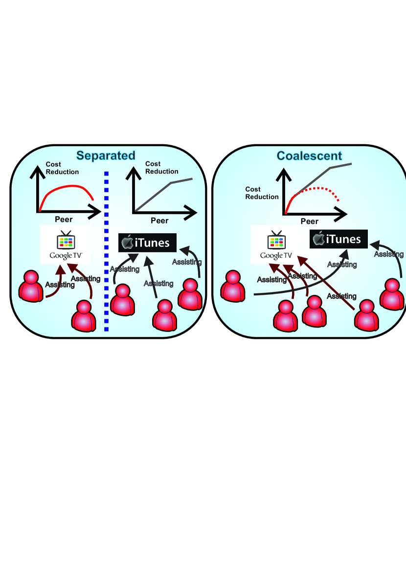
Figure 1: Two coalition structures for a dual-provider peer-assisted service.

However, in practice, the Internet consists of multiple content providers, even if only giant providers are counted. In the multi-provider setting, users and providers are coupled in a more complex manner, thus the model becomes much more challenging and even the cooperative game theoretic framework itself is unclear, e.g., definition of the worth of a coalition. Also, the results and their implications in the multi-provider setting may experience drastic changes, compared to the single-provider case.

The grand coalition is expected to be the “best” coalition in the peer-assisted service with multiple providers in that it provides the highest aggregate payoff. To illustrate, see an example in Fig. 1 with two providers (Google TV and iTunes) and a large number of peers. Consider two cooperation types: (i) separated, where there exists a fixed partition of peers for each provider, and (ii) coalescent, where each peer is possible to assist any provider. In the separated case, a candidate payoff scheme is based on the Shapley value in each disconnected coalition. In the coalescent case, the Shapley value is also a candidate payoff scheme after a worth function of the grand coalition is defined, where a reasonable worth function can be the total optimal profit, maximized over all combinations of peer partitions to each provider. Consequently, the total payoff for the coalescent case exceeds that for the separated case, unless the two partitions of both cases are equivalent. Shapley value is defined by a few agreeable axioms, one of which is efficiency, meaning that the every cent of coalition worth is distributed to players. Since smaller worth is shared out among players in the separated case, at least one individual is underpaid as compared with the coalescent case. Thus, providers and users are recommended to form the grand coalition and be paid off based on the Shapley values.

However, it is still questionable whether peers are willing to stay in the grand coalition and thus the consequent Shapley-value based payoff mechanism is desirable in the multi-provider setting. In this paper, we anatomize incentive structures in peer-assisted services with multiple content providers and focus on stability issues from two different angles: stability at equilibrium of Shapley value and convergence to the equilibrium. We show that the Shapley payoff scheme may lead to unstable coalition structure, and propose a different notion of payoff distribution scheme, $\chi$ value, under which peers and providers stay in the stable coalition as well as better fairness is guaranteed.

I-B Related Work

The research on incentive structure in the P2P systems (e.g., BitTorrent) has been studied extensively. To incapacitate free-riders in P2P systems, who only download contents but upload nothing, from behaving selfishly, a number of incentive mechanisms suitable for distribution of copy-free contents have been proposed (See [5] and references therein), using game theoretic approaches. Alternative approaches to exploit the potential of the P2P systems for reducing the distribution (or operational) costs of the copyrighted contents have been recently adopted by [4, 1]. To the best of our knowledge, the work by Misra et al.[4] is the first to study the profit-sharing mechanism (payoff mechanism) of peer-assisted services.

Coalition game theory has been applied to model diverse networking behaviors, where the main focus in most cases (e.g., [4]) was to study the stability of a specific equilibrium i.e., the grand coalition in connection with the notion of core. Recently, Saad et al.[6, 7], discussed the stability and dynamics of endogenous formation of general coalition structures. In particular, [7] introduced a coalition game model for self-organizing agents (e.g., unmanned aerial vehicles) collecting data from arbitrarily located tasks in wireless networks and proved the stability of the proposed algorithm by using hedonic preference (and dominance). In this paper, we use the stability notion by Hart and Kurz [8] (see also [9]) to study the dynamics of coalition structures in peer-assisted services. The stability notion in [8] is based on the preferences of any arbitrary coalition while the hedonic coalition games are based on the preferences of individuals. Other subtle differences are described in [10].

I-C Main Contributions and Organization

We summarize our main contributions as follows:

1. Following the preliminaries in Section II, in Section III, we describe and propose the cooperative game theoretic framework of the peer-assisted service with multiple providers. After defining a worth function that is provably the unique feasible worth function satisfying two essential properties, i.e., feasibility and superadditivity of a coalition game, we provide a closed-form formula of the Shapley value for a general coalition with multiple providers and peers, where we take a fluid-limit approximation for mathematical tractability. This is a non-trivial generalization of the Shapley value for the single-provider case in [4]. In fact, our formula in Theorem 1 establishes the general Shapley value for distinguished multiple atomic players and infinitesimal players in the context of the Aumann-Shapley (A-S) prices [11] in coalition game theory.

2. In Section IV, we discuss in various ways that the Shapley payoff regime cannot incentivize rational players to form the grand coalition, implying that fair profit-sharing and opportunism of players cannot stand together. First, we prove that the Shapley value for the multiple-provider case is not in the core under mild conditions, e.g., each provider’s cost function is concave. This is in stark contrast to the single-provider case where the concave cost function stabilizes the equilibrium. Second, we study the dynamic formation of coalitions in peer-assisted services by introducing the notion of stability defined by the seminal work of Hart and Kurz [8]. Finally, we show that, if we adopt a Shapley-like payoff mechanism, called Aumann-Drèze value, irrespective of stability of the grand coalition, there always exist initial states which do not converge to the grand coalition.

3. In Section V, we present three examples stating the problems of the non-cooperative peer-assisted service: (i) the peers are underpaid compared to their Shapley payoffs, (ii) a provider paying the highest dividend to peers monopolizes all peers, and (iii) Shapley value for each coalition gives rise to an oscillatory behavior of coalition structures. These examples suggest that the system with the separated providers may be even unstable as well as unfair in a peer-assisted service market.

4. In Section VI, as a partial solution to the problems of Shapley-like payoffs (i.e., Shapley and Aumann-Drèze), we propose an alternative payoff scheme, called $\chi$ value [12]. This payoff mechanism is relatively fair in the sense that players, at the least, apportion the difference between the coalition worth and the sum of their fair shares, i.e., Shapley payoffs, and stabilizes the whole system. It is also practical in the sense that providers are granted a limited right of bargaining. That is, a provider may award an extra bonus to peers by cutting her dividend, competing with other providers in a fair way. More importantly, we show that authorities can effectively avoid unjust rivalries between providers by implementing a simplistic measure.

After presenting a practical example of peer-assisted services with multiple providers in delay-tolerant networks in Section VII, we conclude this paper.

II Preliminaries

Since this paper investigates a multi-provider case, where a peer can choose any provider to assist, we start this section by defining a coalition game with a peer partition (i.e., a coalition structure) and introducing the payoff mechanism thereof.

II-A Game with Coalition Structure

A game with coalition structure is a triple $(N,v,\mathcal{P})$ where $N$ is a player set and $v:2^{N}\rightarrow\R$ ($2^{N}$ is the set of all subsets of $N$) is a worth function, $v(\emptyset)=0$. $v(K)$ is called the worth of a coalition $K\subseteq N$. $\mathcal{P}$ is called a coalition structure for $(N,v)$; it is a partition of $N$ where $C(i)\in\mathcal{P}$ denotes the coalition containing player $i$. For your reference, a coalition structure $\mathcal{P}$ can be regarded as a set of disjoint coalitions. The grand coalition is the partition $\mathcal{P}=\{N\}$. For instance, a partition of $N=\{1,2,3,4,5\}$ is $\mathcal{P}=\{\{1,2\},\{3,4,5\}\},$ $C(4)=\{3,4,5\},$ and the grand coalition is $\mathcal{P}=\{\{1,2,3,4,5\}\}$. $\mathcal{P}(S)$ is the set of all partitions of $S\subseteq N$. For notational simplicity, a game without coalition structure $(N,v,\{N\})$ is denoted by $(N,v)$. A value of player $i$ is an operator $\phi_{i}(N,v,\mathcal{P})$ that assigns a payoff to player $i$. We define $\phi_{K}=\sum_{i\in K}\phi_{i}$ for all $K\subseteq N$.

To conduct the equilibrium analysis of coalition games, the notion of core has been extensively used to study the stability of grand coalition $\mathcal{P}=\{N\}$:

Definition 1 (Core).

The core of a game $(N,v)$ is defined by:

$$\bigg{\{}\phi(N,v)~{}|~{}\sum_{i\in N}\phi_{i}(N,v)=v(N)\cr\mbox{ and }\sum_{i\in K}\phi_{i}(N,v)\geq v(K),\forall K\subseteq N\bigg{\}}.$$

If a payoff vector $\phi(N,v)$ lies in the core, no player in $N$ has an incentive to split off to form another coalition $K$ because the worth of the coalition $K$, $v(K)$, is no more than the payoff sum $\sum_{i\in K}\phi_{i}(N,v)$. Note that the definition of the core hypothesizes that the grand coalition is already formed ex-ante. We can see the core as an analog of Nash equilibrium from noncooperative games. Precisely speaking, it should be viewed as an analog of strong Nash equilibrium where no arbitrary coalition of players can create worth which is larger than what they receive in the grand coalition. If a payoff vector $\phi(N,v)$ lies in the core, then the grand coalition is stable with respect to any collusion to break the grand coalition.

II-B Shapley Value and Aumann-Drèze Value

On the premise that the player set is not partitioned, i.e., $\mathcal{P}=\{N\}$, the Shapley value, denoted by $\varphi$ (not $\phi$), is popularly used as a fair distribution of the grand coalition’s worth to individual players, defined by:

$$\textstyle\varphi_{i}(N,v)\!=\!\!\displaystyle\sum_{S\subseteq N\setminus\{i\}}\textstyle\frac{|S|!(|N|-|S|-1)!}{|N|!}\left(v(S\cup\{i\})\!-\!v(S)\right).$$ (1)

Shapley [13] gives the following interpretation: “(i) Starting with a single member, the coalition adds one player at a time until everybody has been admitted. (ii) The order in which players are to join is determined by chance, with all arrangements equally probable. (iii) Each player, on his admission, demands and is promised the amount which his adherence contributes to the value of the coalition.” The Shapley value quantifies the above that is axiomatized (see Section II-C) and has been treated as a worth distribution scheme. The beauty of the Shapley value lies in that the payoff “summarizes” in one number all the possibilities of each player’s contribution in every coalition structure.

Given a coalition structure $\mathcal{P}\neq\{N\}$, one can obtain the Aumann-Drèze value (A-D value) [14] of player $i$, also denoted by $\varphi$, by taking $C(i)$, which is the coalition containing player $i$, to be the player set and by computing the Shapley value of player $i$ of the reduced game $(C(i),v)$. It is easy to see that the A-D value can be construed as a direct extension of the Shapley value to a game with coalition structure. Note that both Shapley value and A-D value are denoted by $\varphi$ because the only difference is the underlying coalition structure $\mathcal{P}$.

II-C Axiomatic Characterizations of Values

We provide here an axiomatic characterization of the Shapley value [13].

Axiom 1 (Coalition Efficiency, CE).

$\sum_{j\in C}\phi_{j}(N,v,\mathcal{P})=v(C),~{}\forall C\in\mathcal{P}$.

Axiom 2 (Coalition Restricted Symmetry, CS).

If $j\in C(i)$ and $v(K\cup\{i\})=v(K\cup\{j\})$ for all $K\subseteq N\setminus\{i,j\}$, then $\phi_{i}(N,v,\mathcal{P})=\phi_{j}(N,v,\mathcal{P})$.

Axiom 3 (Additivity, ADD).

For all coalition functions $v$, $v^{\prime}$ and $i\in N$, $\phi_{i}(N,v+v^{\prime},\mathcal{P})=\phi_{i}(N,v,\mathcal{P})+\phi_{i}(N,v^{\prime},\mathcal{P})$.

Axiom 4 (Null Player, NP).

If $v(K\cup\{i\})=v(K)$ for all $K\subseteq N$, then $\phi_{i}(N,v,\mathcal{P})=0$.

Recall that the basic premise of the Shapley value is that the player set is not partitioned, i.e., $\mathcal{P}=\{N\}$. It is well-known [12, 13] that the Shapley value, defined in (1), is uniquely characterized by CE, CS, ADD and NP for $\mathcal{P}=\{N\}$. The A-D value is also uniquely characterized by CE, CS, ADD and NP (Axioms 1-4), but in this case for arbitrary coalition structure $\mathcal{P}$ [14]. In the literature, e.g., [6, 15], the A-D value has been used to analyze the static games where a coalition structure is exogenously given.

Definition 2 (Coalition Independent, CI).

If $i\in C\subseteq N$, $C\in\mathcal{P}$ and $C\in\mathcal{P}^{\prime}$, then $\phi_{i}(N,v,\mathcal{P})=\phi_{i}(N,v,\mathcal{P}^{\prime})$.

From the definition of the A-D value, the payoff of player $i$ in coalition $C(i)$ is affected neither by the player set $N$ nor by coalitions $C\in\mathcal{P}$, $C\neq C(i)$. Note that only $C(i)$ contains the player $i$. Thus, it is easy to prove that the A-D value is coalition independent. From CI of the A-D value, in order to decide the payoffs of a game with general coalition structure $\mathcal{P}$, it suffices to decide the payoffs of players within each coalition, say $C\in\mathcal{P}$, without considering other coalitions $C\in\mathcal{P}$, $C\neq C(i)$. In other words, once we decide the payoffs of a coalition $C\in\mathcal{P}$, the payoffs remain unchanged even though other coalitions, $C^{\prime}\in\mathcal{P}$, $C^{\prime}\neq C$, vary. Thus, for any given coalition structure $\cal P$, any coalition $C\in\mathcal{P}$ is just two-fold in terms of the number of providers in $C$: (i) one provider or (ii) two or more providers, as depicted in Fig. 1.

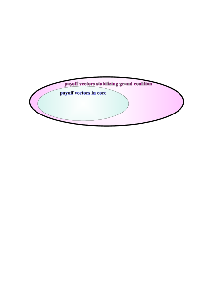
Figure 2: If a payoff vector lies in the core, the grand coalition is stable [8].

Yet another reason why CI attracts our attention is that it enables us to define the stability of a game with coalition structure in the following simplistic way:

Definition 3 (Stable Coalition Structure [8]).

We say that a coalition structure $\mathcal{P}^{\prime}$ blocks $\mathcal{P}$, where $\mathcal{P}^{\prime}$, $\mathcal{P}\in\mathcal{P}(N)$, with respect to $\phi$ if and only if there exists some $C\in\mathcal{P}^{\prime}$ such that $\phi_{i}(N,v,\{C,\cdots\})>\phi_{i}(N,v,\mathcal{P})$ for all $i\in C$. In this case, we also say that $C$ blocks $\mathcal{P}$. If there does not exist any $\mathcal{P}^{\prime}$ which blocks $\mathcal{P}$, $\mathcal{P}$ is called stable.

Due to CI of the A-D value, all stability notions defined by the seminal work of Hart and Kurz [8] coincide with the above simplistic definition, as discussed by Tutic [9]. Definition 3 can be intuitively interpreted that, if there exists any subset of players $C$ who improve their payoffs away from the current coalition structure, they will form a new coalition $C$. In other words, if a coalition structure $\mathcal{P}$ has any blocking coalition $C$, some rational players will break $\mathcal{P}$ to increase their payoffs. The basic premise here is that players are not clairvoyant, i.e., they are interested only in improving their instant payoffs in a myopic way. If a payoff vector lies in the core, the grand coalition is stable in the sense of Definition 3, but the converse is not necessarily true (see Fig. 2).

II-D Comparison with Other Values

In a particular category of games, called voting games or simple games, Banzhaf value as well as the Shapley value (also known as Shapley-Shubik index in this context) has been used in the literature (See, e.g., [16] and references therein). While the Shapley value has been extensively studied in many papers, there are no similar results for the Banzhaf value. For instance, the Shapley value is proven to lie in the core for a special type of games, called convex games, whereas there is no equivalent result for the Banzhaf value. Moreover, the Banzhaf value violates the efficiency axiom CE in Section II-C for a certain coalition structure $\mathcal{P}=\{N\}$, leading to inefficient sharing of the grand coalition worth.

As compared with Aumann-Drèze value, a new value, referred to as Owen value (See, e.g., [15, Chapter 8.8] or [17, Chapter XII]) has emerged based on an alternative viewpoint on coalition, where a coalition forms not to share the coalition worth, but only to maximize their bargaining power with regard to division of the worth of the grand coalition. In other words, players form a labor union (coalition) to obtain a better bargaining position leading to a larger payoff, implying that the coalition efficiency axiom CE is also violated. A delicate premise of this approach is that players must form the grand coalition, the worth of which is in fact the largest worth in superadditive games (See Definition 5), and bargain with each other at the same time. Also, in the context of P2P systems, whether it is more reasonable to nullify CE so that a portion of a worth of a coalition (peers and providers) $C\in\mathcal{P}$ becomes transferrable to other coalitions $C^{\prime}\in\mathcal{P}$, $C\neq C^{\prime}$, remains an open economic question.

III Coalition Game in Peer-Assisted Services

In this section, we first define a coalition game in a peer-assisted service with multiple content providers by classifying the types of coalition structures as separated, where a coalition includes only one provider, and coalescent, where a coalition is allowed to include more than one providers (see Fig. 1). To define the coalition game, we will define a worth function of an arbitrary coalition $S\subseteq N$ for such two cases.

III-A Worth Function in Peer-Assisted Services

Assume that players $N$ are divided into two sets, the set of content providers ${Z}\mathrel{:=}\{p_{1},\cdots,p_{\zeta}\}$, and the set of peers $H\mathrel{:=}\{n_{1},\cdots,n_{\eta}\}$, i.e., $N={Z}\cup H$. We also assume that the peers are homogeneous, e.g., the same computing powers, disk cache sizes, and upload bandwidths. Later, we discuss that our results can be readily extended to nonhomogeneous peers. The set of peers assisting providers is denoted by $\bar{H}\subseteq H$ where $x\mathrel{:=}|\bar{H}|/\eta$, i.e., the fraction of assisting peers. We define the worth of a coalition $S$ to be the amount of cost reduction due to cooperative distribution of the contents by the players in $S$ in both separated and coalescent cases.

Separated case: Denote by $\Omega_{p}^{\eta}(x(S))$ the operational cost of a provider $p$ when the coalition $S$ consists of a single provider $p$ and $x(S)\cdot\eta$ assisting peers. Since the operational cost cannot be negative and may decrease with the number of assisting peers, we assume the following to simplify the exposition:

• Assumption: $\Omega_{p}^{\eta}(x)$ is non-increasing in $x$ for all $p\in{Z}$.

Note that from the homogeneity assumption of peers, the cost function depends only on the fraction of assisting peers. Then, we define the worth function $\hat{v}(S)$ for a coalition $S$ having a single provider as:

$$\hat{v}(S)\mathrel{:=}\Omega_{p}^{\eta}(0)-\Omega_{p}^{\eta}(x(S))$$ (2)

where $\Omega_{p}^{\eta}(0)$ corresponds to the cost when there are no assisting peers. For a coalition $S$ with no provider, we simply have $\hat{v}(S)\mathrel{:=}0.$ For notational simplicity, $x(S)$ is henceforth denoted by $x,$ unless confusion arises.

Coalescent case: In contrast to the separated case, where a coalition includes a single provider, the worth for the coalescent case is not clear yet, since depending on which peers assist which providers the amount of cost reduction may differ. One of reasonable definitions would be the maximum worth out of all peer partitions, i.e., the worth for the coalescent case is defined by: for a coalition with at least two providers,

$$\textstyle v(S)\!\mathrel{:=}\!\max\!\left\{\!\displaystyle{\sum_{C\in\mathcal{P}}}\hat{v}(C)\Big{|}{\mathcal{P}\!\in\!\mathcal{P}(S)}\!\!~{}\mbox{ s.t. }|Z\!\cap\!C|\!=\!1,~{}\forall C\!\in\!\mathcal{P}\!\right\},$$ (3)

and $v(S)\mathrel{:=}\hat{v}(S)$ for a coalition $S$ with at most one provider. The definition above implies that we view a coalition containing more than one provider as the most productive coalition whose worth is maximized by choosing the optimal partition $\mathcal{P}^{*}$ among all possible partitions of $S$. Note that (3) is consistent with the definition (2) for $|{Z}\cap S|=1$, i.e., $v(S)=\hat{v}(S)$ for $|{Z}\cap S|=1$.

Five remarks are in order. First, as opposed to [4] where $\hat{v}(\{p\})=\eta R-\Omega_{p}^{\eta}(0)$ ($R$ is the subscription fee paid by any peer), we simply assume that $\hat{v}(\{p\})=0$. Note that, as discussed in [15, Chapter 2.2.1], it is no loss of generality to assume that, initially, each provider has earned no money. In our context, this means that it does not matter how much fraction of peers is subscribing to each provider because each peer has already paid the subscription fee to providers ex-ante.

Second, $\Omega_{p}^{\eta}(x)$ may not be decreasing because, for example, electricity expense of the computers and the maintenance cost of the hard disks of peers may exceed the cost reduction due to peers’ assistance in content distribution, e.g., Annualized Failure Rate (AFR) of hard disk drives is over 8.6% for three-year old ones [18].

Third, the worth function in peer-assisted services can reflect the diversity of peers. It is not difficult to extend our result to the case where peers belong to distinct classes. For example, peers may be distinguished by different upload bandwidths and different hard disk cache sizes. A point at issue for the multiple provider case is whether peers who are not subscribing to the content of a provider may be allowed to assist the provider or not. On the assumption that the content is ciphered and not decipherable by the peers who do not know its password which is given only to the subscribers, providers will allow those peers to assist the content distribution. Otherwise, we can easily reflect this issue by dividing the peers into a number of classes where each class is a set of peers subscribing to a certain content.

Fourth, it should be clearly understood that our worth function (3) does not encompass more than just the peer-partition optimization. That is, we speculate that cooperation among providers might lead to further expenses cut by optimizing their network resources. We recognize the lack of this ‘added bonus’ to be the major weakness in our model.

Lastly, it should be noted that the worth function in (3) is selected in order to satisfy two properties. First of all, it follows from the definition of $v$ in (3) that no other coalition function $v^{\prime}(\cdot)$ can be greater than $v(\cdot)$, i.e., $v(\cdot)\geq v^{\prime}(\cdot)$ because $v$ is the total cost reduction that is maximized over all possible peer partitions to each provider.

Definition 4 (Feasibility).

For all worth function $v^{\prime}(\cdot)$, we have $v(S)\geq v^{\prime}(S)$ for all $S\subseteq N$.

The second property, superadditivity, is one of the most elementary properties, which ensures that the core is nonempty by appealing to Bondareva-Shapley Theorem [15, Theorem 3.1.4].

Definition 5 (Superadditivity).

A worth $v$ is superadditive if $\left(S,T\subseteq N\mbox{ and }S\cap T=\emptyset\right)\Rightarrow v(S\cup T)\geq v(S)+v(T)$.

The following lemma holds by the fact that a feasible worth function cannot be greater than (3), i.e., the largest worth.

Lemma 1.

When the worth for the separated case is given by (2), for the coalescent case, there exists a unique worth function that is both superadditive and feasible, given by (3).

Proof.

Suppose we have a superadditive worth $v^{\prime}$. Firstly, it follows directly from the assumption (the worth function for the separate case is (2)) that $v^{\prime}(S)=\hat{v}(S)$ if $S$ includes one provider. (i) Feasibility: It follows from the definition of feasibility that we have $v(\cdot)\geq v^{\prime}(\cdot)$ because $v(S)$ is the maximum over all possible partitions $\mathcal{P}\in\mathcal{P}(S)$. (ii) Superadditivity: In the meantime, since $v^{\prime}$ is superadditive, it must satisfy $v^{\prime}(S\cup T)\geq v^{\prime}(S)+v^{\prime}(T)$ for all disjoint $S$, $T\subseteq N$. This in turn implies $v^{\prime}(S)\geq\sum_{C\in\mathcal{P}}v^{\prime}(C)$ for all $\mathcal{P}$ such that $\mathcal{P}\in\mathcal{P}(S)$. The right-hand side $\sum_{C\in\mathcal{P}}v^{\prime}(C)$ should coincide with $v(S)$ for some $\mathcal{P}=\mathcal{P}^{*}$ such that $|{Z}\cap C|=1$ for all $C\in\mathcal{P}^{*}$ (See (3)), where $\mathcal{P}^{*}$ is the peer partition which maximizes $v(S)$. Therefore, we have $v^{\prime}(S)\geq v(S)$. Combining this with $v(\cdot)\geq v^{\prime}(\cdot)$ uniquely determines $v^{\prime}(\cdot)=v(\cdot)$.

In light of this lemma, we can restate that our objective in this paper is to analyze the incentive structure of peer-assisted services when the worth of coalition is feasible and superadditive. This objective in turn implies the form of worth function in (3).

$$\left\{\begin{array}[]{ll}\widetilde{\varphi}_{p}^{{\bar{Z}}}(x)=\widetilde{\Omega}_{p}(0)-\sum_{S\subseteq{\bar{Z}}\setminus\{p\}}\int_{0}^{1}u^{|S|}(1-u)^{|{\bar{Z}}|-1-|S|}\left(M_{\Omega}^{S\cup\{p\}}(ux)-M_{\Omega}^{S}(ux)\right)\mathrm{d}u,&\mbox{for }p\in{\bar{Z}}\\ \widetilde{\varphi}_{n}^{{\bar{Z}}}(x)=-\sum_{S\subseteq{\bar{Z}}}\int_{0}^{1}u^{|S|}(1-u)^{|{\bar{Z}}|-|S|}\frac{\mathrm{d}M_{\Omega}^{S}}{\mathrm{d}x}(ux)\mathrm{d}u,&\mbox{for }n\in\bar{H}.\end{array}\right.$$ (FluidAD1)

$$\left\{\begin{array}[]{ll}\widetilde{\varphi}_{p}^{\{p,q\}}(x)={\widetilde{\Omega}}_{p}(0)-\int_{0}^{1}uM_{\Omega}^{\{p,q\}}(ux)\mathrm{d}u-\int_{0}^{1}(1-u)M_{\Omega}^{\{p\}}(ux)\mathrm{d}u+\int_{0}^{1}uM_{\Omega}^{\{q\}}(ux)\mathrm{d}u,&\mbox{(}p,~{}q\mbox{ are interchangeable)}\\ \widetilde{\varphi}_{n}^{\{p,q\}}(x)=-\int_{0}^{1}u^{2}\frac{\mathrm{d}M_{\Omega}^{\{p,q\}}}{\mathrm{d}x}(ux)\mathrm{d}u-\sum_{i\in\{p,q\}}\int_{0}^{1}u(1-u)\frac{\mathrm{d}M_{\Omega}^{\{i\}}}{\mathrm{d}x}(ux)\mathrm{d}u,&\mbox{for }n\in\bar{H}.\end{array}\right.$$ (FluidAD2)

Figure 3: Fluid Aumann-Drèze payoff formula for multi-provider coalitions, construed as an extension of Aumann-Shapley prices to multiple atomic players.

III-B Fluid Aumann-Drèze Value for Multi-Provider Coalitions

So far we have defined the worth of coalitions. Now let us distribute the worth to the players for a given coalition structure $\mathcal{P}$. Recall that the payoffs of players in a coalition are independent from other coalitions by the definition of A-D payoff. Pick a coalition $C$ without loss of generality, and denote the set of providers in $C$ by $\bar{Z}\subseteq Z$. With slight notational abuse, the set of peers assisting $\bar{Z}$ is denoted by $\bar{H}$. Once we find the A-D payoff for a coalition consisting of arbitrary provider set ${\bar{Z}}\subseteq Z$ and assisting peer set $\bar{H}\subseteq H$, the payoffs for the separated and coalescent cases in Fig. 1 follow from the substitutions $\bar{Z}=Z$ and $\bar{Z}=\{p\}$, respectively. In light of our discussion in Section II-B, it is more reasonable to call a Shapley-like payoff mechanism ‘A-D payoff’ and ‘Shapley payoff’ respectively for the partitioned and non-partitioned games $(N,v,\{{\bar{Z}}\cup\bar{H},\cdots\})$ and $(N,v,\{Z\cup H\})$.

Fluid Limit: We adopt the limit axioms for a large population of users to overcome the computational hardness of the A-D payoffs:

$$\textstyle\lim_{\eta\to\infty}\widetilde{\Omega}_{p}^{\eta}(\cdot)=\widetilde{\Omega}_{p}(\cdot)~{}~{}\mbox{ where }\widetilde{\Omega}_{p}^{\eta}(\cdot)=\frac{1}{\eta}{\Omega}_{p}^{\eta}(\cdot)$$ (4)

which is the asymptotic operational cost per peer in the system with a large number of peers. We drop superscript $\eta$ from notations to denote their limits as $\eta\to\infty$. From the assumption $\Omega_{p}^{\eta}(x)>0$, we have $\widetilde{\Omega}_{p}(x)\geq 0$. To avoid trivial cases, we also assume ${\widetilde{\Omega}}_{p}(x)$ is not constant in the interval $x\in[0,1]$ for any $p\in{Z}$. We also introduce the payoff of each provider per user, defined as $\widetilde{\varphi}^{\eta}_{p}\mathrel{:=}\frac{1}{\eta}\varphi^{\eta}_{p}$. We now derive the fluid limit equations of the payoffs, shown in Fig. 3, which can be obtained as $\eta\to\infty$. The proof of the following theorem is given in Appendix A-A.

Theorem 1 (A-D Payoff for Multiple Providers).

As $\eta\to\infty$, the A-D payoffs of providers and peers under an arbitrary coalition $C=\bar{Z}\cup\bar{H}$ converge to (FluidAD1) in Fig. 3 where $M_{\Omega}^{S}(x)\mathrel{:=}\min\left\{\sum_{i\in S}\widetilde{\Omega}_{i}(y_{i})~{}\big{|}~{}\sum_{i\in S}y_{i}\leq x,~{}y_{i}\geq 0\right\}$ and $M_{\Omega}^{\emptyset}(x)\mathrel{:=}0$. Note that $M_{\Omega}^{\{p\}}(x)={\widetilde{\Omega}}_{p}(x)$.

The following corollaries are immediate as special cases of Theorem 1, which we will use in Section V.

Corollary 1 (A-D Payoff for Single Provider).

As $\eta\to\infty$, the A-D payoffs of providers and peers who belong to a single-provider coalition, i.e., ${\bar{Z}}=\{p\}$, converge to:

$$\left\{\begin{array}[]{ll}\widetilde{\varphi}_{p}^{\{p\}}(x)={\widetilde{\Omega}}_{p}(0)-\int_{0}^{1}M_{\Omega}^{\{p\}}(ux)\mathrm{d}u,&\\ \widetilde{\varphi}_{n}^{\{p\}}(x)=-\int_{0}^{1}u\frac{\mathrm{d}M_{\Omega}^{\{p\}}}{\mathrm{d}x}(ux)\mathrm{d}u,&\mbox{for }n\in\bar{H}.\end{array}\right.$$ (5)

Corollary 2 (A-D Payoff for Dual Providers).

As $\eta\to\infty$, the A-D payoffs of providers and peers who belong to a dual-provider coalition, i.e., ${\bar{Z}}=\{p,q\}$, converge to (FluidAD2).

Note that our A-D payoff formula in Theorem 1 generalizes the formula in Misra et al.[4, Theorem 4.3] (i.e., $|{Z}|=1$). It also establishes the A-D values for distinguished multiple atomic players (the providers) and infinitesimal players (the peers), in the context of the Aumann-Shapley (A-S) prices [11] in coalition game theory.

Our formula for the peers is interpreted as follows: Take the second line of (FluidAD2) as an example. Recall the definition of the Shapley value (1). The payoff of peer $n$ is the marginal cost reduction $v(S\cup\{n\})-v(S)$ that is averaged over all equally probable arrangements, i.e., the orders of players. It is also implied by (1) that the expectation of the marginal cost is computed under the assumption that the events $|S|=y$ and $|S|=y^{\prime}$ for $y\neq y^{\prime}$ are equally probable, i.e., $\textsf{P}(|S|=y)=\textsf{P}(|S|=y^{\prime})$. Therefore, in our context of infinite player game in Theorem 1, for every values of $ux$ along the interval $[0,x]$, the subset $S\subseteq{\bar{Z}}\cup\bar{H}$ contains $ux$ fraction of the peers. More importantly, the probability that each provider is a member of $S$ is simply $u$ because the size of peers in $S$, $\eta ux$, is infinite as $\eta\to\infty$ so that the size of $S$ is not affected by whether a provider belongs to $S$ or not. Therefore, the marginal cost reduction of each peer on the condition that both providers are contained in $S$ becomes $-u^{2}\frac{\mathrm{d}M_{\Omega}^{\{p,q\}}}{\mathrm{d}x}(ux)$. Likewise, the marginal cost reduction of each peer on the condition that only one provider is in the coalition is $-u(1-u)\frac{\mathrm{d}M_{\Omega}^{\{p\}}}{\mathrm{d}x}(ux)$.

IV Instability of the Grand Coalition

In this section, we study the stability of the grand coalition to see if rational players are willing to form the grand coalition, only under which they can be paid their respective fair Shapley payoffs. The key message of this section is that the rational behavior of the providers makes the Shapley value approach unworkable because the major premise of the Shapley value, the grand coalition, is not formed in the multi-provider games.

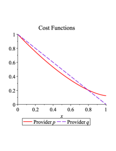
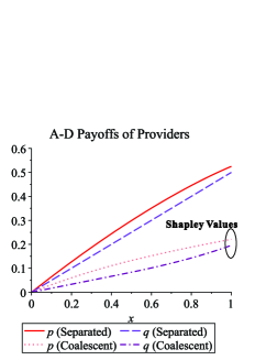
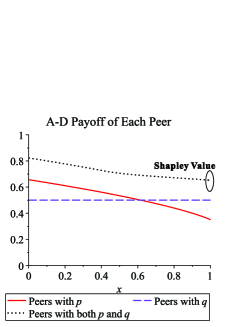
Figure 4: Example 1: A-D Payoffs of Two Providers and Peers for Convex Cost Functions.

IV-A Stability of the Grand Coalition

Guaranteeing the stability of a payoff vector has been an important topic in coalition game theory. For the single-provider case, $|{Z}|=1$, it was shown in [4, Theorem 4.2] that, if the cost function is decreasing and concave, the Shapley incentive structure lies in the core of the game. What if for $|{Z}|\geq 2$? Is the grand coalition stable for the multi-provider case? Prior to addressing this question, we first define the following:

Definition 6 (Noncontributing Provider).

A provider $p\in{Z}$ is called noncontributing if $M_{\Omega}^{Z}(1)-M_{\Omega}^{{Z}\setminus\{p\}}(1)={\widetilde{\Omega}}_{p}(0)$.

To understand this better, note that the above expression is equivalent to the following:

$$\textstyle\displaystyle\sum_{i\in{Z}}\textstyle{\widetilde{\Omega}}_{i}(0)-M_{\Omega}^{Z}(1)=\displaystyle\sum_{i\in{Z}\setminus\{p\}}\textstyle{\widetilde{\Omega}}_{i}(0)-M_{\Omega}^{{Z}\setminus\{p\}}(1)$$ (6)

which implies that there is no difference in the total cost reduction, irrespective of whether the provider $p$ is in the provider set or not. Interestingly, if all cost functions are concave, there exists at least one noncontributing provider.

Lemma 2.

Suppose $|{Z}|\geq 2$. If ${\widetilde{\Omega}}_{p}(\cdot)$ is concave for all $p\in{Z}$, there exist $|Z|-1$ noncontributing providers.

To prove this, recall the definition of $M_{\Omega}^{Z}(\cdot)$:

$$\textstyle M_{\Omega}^{{Z}}(x)=\min_{y\in Y(x)}\sum_{i\in{Z}}{\widetilde{\Omega}}_{i}(y_{i})$$

$$\textstyle\mbox{where}~{}Y(x)\mathrel{:=}\{(y_{1},\cdots,y_{|{Z}|})~{}\big{|}~{}\sum_{i\in{Z}}y_{i}\leq x,~{}y_{i}\geq 0\}.$$

Since the summation of concave functions is concave and the minimum of a concave function over a convex feasible region $Y(x)$ is an extreme point of $Y(x)$ as shown in [19, Theorem 3.4.7], we can see that the solutions of the above minimization are the extreme points of $\{(y_{1},\cdots,y_{|{Z}|})~{}|~{}\sum_{i\in{Z}}y_{i}\leq x,~{}y_{i}\geq 0\}$, which in turn imply $y_{i}=0$ for $|Z|-1$ providers in $Z$. Note that the condition $|Z|\geq 2$ is necessary here.

We are ready to state the following theorem, a direct consequence of Theorem 1. Its proof is in Appendix A-B.

Theorem 2 (Shapley Payoff Not in the Core).

If there exists a noncontributing provider, the Shapley payoff for the game $({Z}\cup H,v)$ does not lie in the core.

It follows from Lemma 2 that, if all operational cost functions are concave and $|{Z}|\geq 2$, the Shapley payoff does not lie in the core. This result appears to be in good agreement with our usual intuition. If there is a provider who does not contribute to the coalition at all in the sense of (6) and is still being paid due to her potential for imaginary contribution assessed by the Shapley formula (1), which is not actually exploited in the current coalition, other players may improve their payoff sum by expelling the noncontributing provider.

The condition $|{Z}|\geq 2$ plays an essential role in the theorem. For $|{Z}|\geq 2$, the concavity of the cost functions leads to the Shapley value not lying in the core, whereas, for the case $|{Z}|=1$, the concavity of the cost function is proven to make the Shapley incentive structure lie in the core [4, Theorem 4.2].

IV-B Convergence to the Grand Coalition

The notion of the core lends itself to the stability analysis of the grand coalition on the assumption that the players are already in the equilibrium, i.e., the grand coalition. However, Theorem 2 still leaves further questions unanswered. In particular, for the non-concave cost functions, it is unclear if the Shapley value is not in the core, which is still an open problem. We rather argue here that, whether the Shapley value lies in the core or not, the grand coalition is unlikely to occur by showing that the grand coalition is not a global attractor under some conditions.

To study the convergence of a game with coalition structure to the grand coalition, let us recall Definition 3. It is interesting that, though the notion of stability was not used in [4], one main argument of this work was that the system with one provider would converge to a full sharing mode, i.e., the grand coalition, hinting the importance of the following convergence result with multiple providers. The proof of the following theorem is given in Appendix A-C.

Theorem 3 (A-D Payoff Doesn’t Lead to Grand Coalition).

Suppose $|{Z}|\geq 2$ and ${\widetilde{\Omega}}_{p}(y)$ is not constant in the interval $y\in[0,x]$ for any $p\in{Z}$ where $x=|\bar{H}|/|H|$. The following holds for all $p\in{Z}$ and $n\in\bar{H}$.

• The A-D payoff of provider $p$ in coalition $\{p\}\cup\bar{H}$ is larger than that in all coalition $T\cup\bar{H}$ for $\{p\}\subsetneq T\subseteq{Z}$.

• The A-D payoff of peer $n$ in coalition $\{p\}\cup\bar{H}$ is smaller than that in all coalition $T\cup\bar{H}$ for $\{p\}\subsetneq T\subseteq{Z}$.

In plain words, a provider, who is in cooperation with a peer set, will receive the highest dividend when she cooperates only with the peers excluding other providers whereas each peer wants to cooperate with as many as possible providers. It is surprising that, for the multiple provider case, i.e., $|{Z}|\geq 2$, each provider benefits from forming a single-provider coalition whether the cost function is concave or not. There is no positive incentives for providers to cooperate with each other under the implementation of A-D payoffs. On the contrary, a peer always looses by leaving the grand coalition.

Upon the condition that each provider begins with a single-provider coalition with a sufficiently large number of peers, one cannot reach the grand coalition because some single-provider coalitions are already stable in the sense of the stability in Definition 3. That is, the grand coalition is not the global attractor. For instance, take $\mathcal{P}=\{\{p\}\cup H,\cdots\}$ as the current coalition structure where all peers are possessed by provider $p$. Then it follows from Theorem 3 that players cannot make any transition from $\mathcal{P}$ to $\{\Phi\cup H,\cdots\}$ where $\Phi\subseteq Z$ is any superset of $\{p\}$ because provider $p$ will not agree to do so.

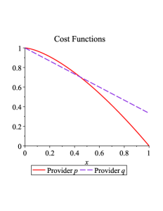
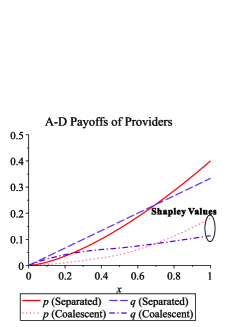
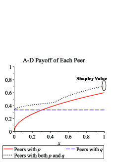
Figure 5: Example 2: A-D Payoffs of Two Providers and Peers for Concave Cost Functions.

V Critique of A-D Payoff for Separate Providers

The discussion so far has focused on the stability of the grand coalition. The result in Theorem 2 suggests that if there is a noncontributing (free-riding) provider, which is true even for concave cost functions for multiple providers, the grand coalition will not be formed. The situation is aggravated by Theorem 3, stating that single-provider coalitions (i.e., the separated case) will persist if providers are rational. We now illustrate the weak points of the A-D payoff under the single-provider coalitions with three representative examples.

V-A Unfairness and Monopoly

Example 1 (Unfairness).

Suppose that there are two providers, i.e., ${Z}=\{p,q\}$, with ${\widetilde{\Omega}}_{p}(x)=7(x-1)^{1.5}/8+1/8$ and ${\widetilde{\Omega}}_{q}(x)=1-x$, both of which are decreasing and convex. All values are shown in Fig. 4 as functions of $x$. In line with Theorem 3, provider $p$ is paid more than her Shapley value, whereas peers are paid less than theirs.

We can see that each peer $n$ will be paid $21/32$ ($\widetilde{\varphi}_{n}^{\{p\}}(0)$) when he is contained by the coalition $\{p,n\}$ and the payoff decreases with the number of peers in this coalition. On the other hand, provider $p$ wants to be assisted by as many peers as possible because $\widetilde{\varphi}_{p}^{\{p\}}(x)$ is increasing in $x$. If it is possible for $n$ to prevent other peers from joining the coalition, he can get $21/32$. However, it is more likely in real systems that no peer can kick out other peers, as discussed in [4, Section 5.1] as well. Thus, $p$ will be assisted by $x=0.6163$ fraction of peers, which is the unique solution of $\widetilde{\varphi}_{n}^{\{p\}}(x)=\widetilde{\varphi}_{n}^{\{q\}}(x)$ while $q$ will be assisted by $1-x=0.3837$ fraction of peers.

Example 2 (Monopoly).

Consider a two-provider system ${Z}=\{p,q\}$ with ${\widetilde{\Omega}}_{p}(x)=1-x^{3/2}$ and ${\widetilde{\Omega}}_{q}(x)=1-2x/3$, both of which are decreasing and concave. Similar to Example 1, we can obtain $\widetilde{\varphi}_{p}^{\{p\}}(x)=2x^{3/2}/5$, $\widetilde{\varphi}_{q}^{\{q\}}(x)=x/3$, $\widetilde{\varphi}_{n}^{\{p\}}(x)=3x^{1/2}/5$ and $\widetilde{\varphi}_{n}^{\{q\}}(x)=1/3$. All values including the Shapley values are shown in Fig. 5. Not to mention unfairness in line with Example 1 and Theorem 3, provider $p$ monopolizes the whole peer-assisted services. No provider has an incentive to cooperate with other provider. It can be seen that all peers will assist provider $p$ because $\widetilde{\varphi}_{n}^{\{p\}}(x)>\widetilde{\varphi}_{n}^{\{q\}}(x)$ for $x>25/81$. Appealing to Definition 3, if the providers are initially separated, the coalition structure will converge to the service monopoly by $p$. In line with Lemma 2 and Theorem 2, even if the grand coalition is supposed to be the initial condition, it is not stable in the sense of the core. The noncontributing provider (Definition 6) in this example is $q$.

V-B Instability of A-D Payoff Mechanism

The last example illustrates the A-D payoff can even induce an analog of the limit cycle in nonlinear systems, i.e., a closed trajectory having the property that other trajectories spirals into it as time approaches infinity.

Example 3 (Oscillation).

Let us consider a game with two providers and two peers where $N=\{p_{1},p_{2},n_{1},n_{2}\}$. If $\{n_{1}\}$, $\{n_{2}\}$ and $\{n_{1},n_{2}\}$ assist the content distribution of $p_{1}$, the reduction of the distribution cost is respectively 10$, 9$ and 11$ per month. However, the hard disk maintenance cost incurred from a peer is 5$. In the meantime, if $\{n_{1}\}$, $\{n_{2}\}$ and $\{n_{1},n_{2}\}$ assist the content distribution of $p_{2}$, the reduction of the distribution cost is respectively 6$, 3$ and 13$ per month. In this case, the hard disk maintenance cost incurred from a peer is supposed to be 2$ due to smaller contents of $p_{2}$ as opposed to those of $p_{1}$.

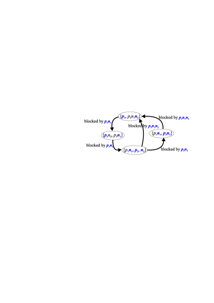
Figure 6: Example 3: A-D Payoff Leads to Oscillatory Coalition Structure.

For simplicity, we omit the computation of the A-D payoffs for all coalition structures and stability analysis (see Appendix of [20] and Table 1 in [20] for details). We first observe that the Shapley payoff of this example does not lie in the core. As time tends to infinity, the A-D payoff exhibits an oscillation of the partition $\mathcal{P}$ consisting of the four recurrent coalition structures as shown in Fig. 6, where, for notational simplicity, we adopt a simplified expression for coalitional structure $\mathcal{P}$: a coalition $\{a,b,c\}\in\mathcal{P}$ is denoted by $abc$ and each singleton set $\{i\}$ is denoted by $i$. The evolution of coalition structure is governed by a simple rule: if there exist blocking coalitions (See Definition 3), then arbitrary one of them will be formed.

Let us begin with the partition $\{p_{1},p_{2}n_{1}n_{2}\}$. Player $p_{1}$ could have achieved the maximum payoff if he had formed a coalition only with $n_{1}$. However, player $n_{1}$ will remain in the current coalition because he does not improve away from the current coalition. Instead, Player $n_{2}$ breaks the coalition $p_{2}n_{1}n_{2}$ so that $n_{2}$ and $p_{1}$ can form coalition $p_{1}n_{2}$ for their benefit. As soon as the coalition $p_{2}n_{1}n_{2}$ is broken, $p_{1}$ betrays $n_{2}$ to increase his payoff by colluding with $n_{1}$. It is not clear how this behavior will be in large-scale systems, as reported in the literature [9].

$$\widetilde{\chi}_{i}^{\bar{Z}}(x) \textstyle=\widetilde{\varphi}_{i}^{Z}(1)+\frac{w_{i}^{\prime}}{x+\sum_{j\in\bar{Z}}w_{j}}\left(\sum_{j\in\bar{Z}}\Omega_{j}(0)-M_{\Omega}^{\bar{Z}}(x)-\left(x\widetilde{\varphi}_{n}^{Z}(1)+\sum_{j\in\bar{Z}}\widetilde{\varphi}_{j}^{Z}(1)\right)\right)~{}\mbox{where }w_{i}^{\prime}=\left\{\begin{array}[]{ll}w_{i},&\mbox{for }i\in\bar{Z},\\ 1,&\mbox{for }i\in\bar{H},\end{array}\right.$$ (FluidChi)

Figure 7: Fluid $\chi$ payoff formula for multi-provider coalitions.

VI A Fair, Bargaining, and Stable Payoff Mechanism for Peer-Assisted Services

The key messages from the examples in Section V imply that the A-D value of the separate case gives rise to unfairness, monopoly, and even oscillation. Also, it turns out that some players’ coalition worth exceeds their Shapley payoffs which they are paid in the grand coalition (Theorem 2). Thus, the Shapley payoff scheme does not seem to be executable in practice because it is impossible to make all players happy, unequivocally. That being said, the fairness of profit-sharing and the opportunism of players are difficult to stand together. Then, it is more reasonable to come up with a compromising payoff mechanism that (i) forces players to apportion the difference between the coalition worth and the sum of their fair shares, (ii) grant providers a limited right of bargaining, and (iii) stabilize the whole system. We will use a slightly different notion of payoff mechanism, called $\chi$ value, originally proposed by Casajus [12].

VI-A An Axiomatic Characterization of $\chi$ Value

The $\chi$ value is characterized by a similar set of axioms used for the A-D value. The only difference is that (i) NP is weakened to GNP, causing a deficiency in axiomatic characterization, which is made up by WSP:

Axiom 5 (Grand Coalition Null Player, GNP).

If $v(K\cup\{i\})=v(K)$ for all $K\subseteq N$, then $\phi_{i}(N,v,\{N\})=0$.

Axiom 6 (Weighted Splitting, WSP).

If $\mathcal{P}^{\prime}$ is finer than $\mathcal{P}$ (i.e., $C^{\prime}(i)\subseteq C(i)$, $\forall i\in N$) and $j\in\mathcal{P}^{\prime}(i)$,

$$\displaystyle\frac{\phi_{i}(N,\!v,\!\mathcal{P})\!-\!\phi_{i}(N,\!v,\!\mathcal{P}^{\prime})}{w_{i}}\!=\!\frac{\phi_{j}(N,\!v,\!\mathcal{P})\!-\!\phi_{j}(N,\!v,\!\mathcal{P}^{\prime})}{w_{j}}.$$

The cornerstone of $\chi$ value is the very observation that, as the grand coalition $\mathcal{P}=\{N\}$ is broken into two or more coalitions, player $i$ now has another option to ally with other coalitions than $C(i)\in\mathcal{P}$ and this outside option must be assessed. To allow the assessment of the outside options, it is inevitable to weaken NP (See Section II-C) to GNP, by satisfying only which, a player may receive positive payoff so far as he contributes to the worth of the grand coalition, even though he does not to that of the current coalition, i.e., NP. In the end, it is all about how to valuate the outside option, the $\chi$ value’s choice of which is to stick to the Shapley value by equally dividing the difference between the coalition worth and the sum of Shapley values, i.e., WSP for $\mathcal{P}=\{N\}$.

Recalling the definition $\varphi_{K}(N,v)=\sum_{i\in K}\varphi_{i}(N,v)$ in Section II-A, we present the following theorem (see [12, 21] for the proof):

Theorem 4 ($\chi$ Value).

The $\chi$ value is uniquely characterized by CE, CS, ADD, GNP and WSP as follows:

$$\chi_{i}(N,v,\mathcal{P})=\varphi_{i}+\frac{w_{i}}{\sum_{k\in C(i)}w_{k}}\left(v(C(i))-\varphi_{C(i)}\right)$$ (7)

where $\varphi_{i}$ is Shapley value of player $i$ for non-partitioned game $(N,v)=(N,v,\{N\})$.

VI-B Fluid $\chi$ Value for Multi-Provider Coalitions

Recall $N=Z\cup H$, $\bar{Z}\subseteq Z$, $\bar{H}\subseteq H$ and $x=|\bar{H}|/\eta$. To compute the $\chi$ payoff for the multiple provider case, we first establish in the following theorem a fluid $\chi$ value in line with the analysis in Section III-B with the limit axioms:

Theorem 5 ($\chi$ Payoff for Multiple Providers).

As $\eta$ tends to infinity, the $\chi$ payoffs of providers and peers under an arbitrary coalition $C=\bar{Z}\cup\bar{H}$ converge to (FluidChi) in Fig. 7 where the Shapley payoffs $\widetilde{\varphi}_{i}^{Z}(1)$ are given in (FluidAD1) in Fig. 3.

To intuitively interpret $\chi$ value, it is crucial to know the roles of Axiom WSP and its weights $w_{i}$. In our context, because of fairness between peers, it is more reasonable to set $w_{i}=1$ for $i\in H$. It does not make sense to differentiate payoffs between peers due to the peer-homogeneity assumption in Section III-A. On the contrary, we will clarify in Sections VI-C and VI-D why the weights of providers $w_{i}$, $i\in Z$ do not necessarily have to be $1$. The essential difference between A-D value and $\chi$ value lies in WSP.

Interpretation of WSP: It implies that, if peer $i$ loses, say $\Delta_{i}$, when the coalition structure changes, e.g., from the grand coalition $\mathcal{P}=\{N\}$ to a finer coalition structure $\mathcal{P}^{\prime}\neq\{N\}$, the provider $p\in C(i)$ will lose $\Delta_{i}\times w_{p}$. There are two implications of this weighted splitting. First, since the payoff of each player $i$ is computed based on the baseline, i.e., the Shapley value, and the surplus or deficit incurred by formation of the coalition $C^{\prime}(i)$ are equally distributed for $w_{p}=1$, $\chi$ value leads to a fair share of the profit. Secondly, now a provider may bargain with peers over the dividend rate by setting $w_{p}$ to any positive number. We elaborate on these two implications in the following subsections.

VI-C Fairness: Surplus-Sharing

On the basis of the first implication of WSP, $\chi$ value is fairer than A-D value in the following sense:

Definition 7 (Surplus-Sharing).

A value $\phi$ of game $(N,v,\mathcal{P})$ is surplus-sharing if the following condition holds: if the coalition worth of coalition $C\in\mathcal{P}$ is greater than, equal to, or less than the sum of Shapley values of players in $C$, i.e., $\sum_{i\in C}\phi_{i}(N,v,\mathcal{P})\gtreqqless\sum_{i\in C}\varphi_{i}(N,v)$, then the payoff of player $i\in C$ is greater than, equal to, or less than the Shapley value of player $i$, respectively, i.e., $\phi_{i}(N,v,\mathcal{P})\gtreqqless\varphi_{i}(N,v)$, for all $i\in C$ and for all $C\in\mathcal{P}$.

Since we proved in Theorem 3 that, for $|Z|\geq 2$, the payoff of provider $p$ in coalition $\{p\}\cup H$ exceeds her Shapley value and that of peer $n\in H$ is smaller than his, it is clear from this definition that A-D value is not surplus-sharing for $|Z|\geq 2$, whereas $\chi$ value is surplus-sharing for any $Z$, e.g., see (7) and (FluidChi). For reference, both A-D and $\chi$ values are surplus-sharing if $|Z|=1$.

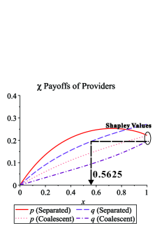
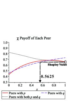
Figure 8: Example 1: $\chi$ Payoffs of Two Providers and Peers for Convex Cost Functions with $w_{p}=w_{q}=1$.

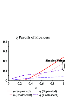
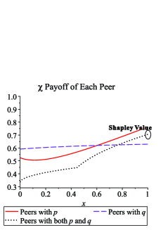
Figure 9: Example 2: $\chi$ Payoffs of Two Providers and Peers for Concave Cost Functions with $w_{p}=w_{q}=1$.

The corresponding $\chi$ payoffs of Examples 1 and 2 for $w_{i}=1$, $\forall i\in Z$, are shown in Figs. 8 and 9. As was the case of the A-D payoffs in Examples 1 and 2, the grand coalitions are not stable. However, due to the surplus-sharing property of the $\chi$ payoff, whenever the coalition worth is larger than the Shapley sum of players in the coalition, all players in the coalition are paid more and vice versa. For instance, we can see from Fig. 8 that if the coalition is formed by provider $q$ and $x>0.5625$ fraction of peers, all members of the coalition are paid more than their respective Shapley payoffs.

As shown in Fig. 9, the monopoly phenomenon of Example 2 for the case of A-D payoff is still observed for the case of $\chi$ value. Regarding Example 1, as shown in Fig. 8, $\chi$ payoff even induces the monopoly by $q$, which did not exist for the case of A-D payoff.

TABLE I: Example 3: $\chi$ Payoff and Blocking Coalition $C$

	$\{p_{1}p_{2},n_{1}n_{2}\}$	$\{p_{1}p_{2},n_{1},n_{2}\}$	$\{p_{1}n_{1},p_{2},n_{2}\}$	$\{p_{1},p_{2},n_{1},n_{2}\}$	$\{p_{1}n_{1},p_{2}n_{2}\}$
$\chi_{p_{1}}$	-1	-1	5/3=1.67	0	5/3=1.67
$\chi_{p_{2}}$	1	1	0	0	7/6=1.17
$\chi_{n_{1}}$	1/2=0.5	0	10/3=3.33	0	10/3=3.33
$\chi_{n_{2}}$	-1/2=-0.5	0	0	0	-1/6=-0.17
$C$	$p_{1}$,$n_{2}$,$p_{1}n_{1}$,$p_{2}n_{2}$,$p_{1}n_{2}$,$p_{2}n_{1}$	$p_{1}$,$p_{1}n_{1}$,$p_{1}n_{2}$,$p_{2}n_{1}$		$p_{1}n_{1}$,$p_{1}n_{2}$,$p_{2}n_{1}$
	$p_{1}p_{2}n_{1}n_{2}$,$p_{1}p_{2}n_{1}$,$p_{1}p_{2}n_{2}$	$p_{1}p_{2}n_{1}n_{2}$,$p_{1}p_{2}n_{1}$,$p_{1}p_{2}n_{2}$	$-$	$p_{1}p_{2}n_{1}n_{2}$,$p_{1}p_{2}n_{1}$,$p_{1}p_{2}n_{2}$	$n_{2}$
	$p_{1}n_{1}n_{2}$,$p_{2}n_{1}n_{2}$,$p_{1}p_{2}n_{1}n_{2}$	$p_{1}n_{1}n_{2}$,$p_{2}n_{1}n_{2}$,$p_{1}p_{2}n_{1}n_{2}$		$p_{2}n_{1}n_{2}$,$p_{1}p_{2}n_{1}n_{2}$
	$\{p_{1}p_{2}n_{2},n_{1}\}$	$\{p_{1}p_{2}n_{1},n_{2}\}$	$\{p_{2}n_{1}n_{2},p_{1}\}$	$\{p_{1}p_{2}n_{1}n_{2}\}$	$\{p_{1}n_{2},p_{2},n_{1}\}$
$\chi_{p_{1}}$	4/9=0.44	4/9=0.44	0	7/6 = 1.17	5/3=1.67
$\chi_{p_{2}}$	22/9=2.44	22/9=2.44	32/9=3.56	19/6 = 3.17	0
$\chi_{n_{1}}$	0	19/9=2.11	29/9=3.22	17/6 = 2.83	0
$\chi_{n_{2}}$	10/9=1.11	0	20/9=2.22	11/6 = 1.83	7/3=2.33
$C$	$p_{1}n_{1}$,$p_{1}p_{2}n_{1}n_{2}$,$p_{2}n_{1}n_{2}$,$p_{1}n_{2}$	$p_{1}n_{1}$,$p_{2}n_{1}n_{2}$,$p_{1}n_{2}$	$p_{1}n_{2}$, $p_{1}n_{1}$	$p_{1}n_{1}$,$p_{2}n_{1}n_{2}$,$p_{1}n_{2}$	$p_{2}n_{1}$
	$\{p_{1}n_{1}n_{2},p_{2}\}$	$\{p_{1},p_{2},n_{1}n_{2}\}$	$\{p_{1},n_{1},p_{2}n_{2}\}$	$\{p_{1},n_{2},p_{2}n_{1}\}$	$\{p_{1}n_{2},p_{2}n_{1}\}$
$\chi_{p_{1}}$	-4/9=-0.44	0	0	0	5/3=1.67
$\chi_{p_{2}}$	0	0	7/6=1.17	13/6=2.17	13/6=2.17
$\chi_{n_{1}}$	11/9=1.22	1/2=0.5	0	11/6=1.83	11/6=1.83
$\chi_{n_{2}}$	2/9=0.22	-1/2=-0.5	-1/6=-0.17	0	7/3=2.33
$C$	$p_{1}$,$p_{1}n_{1}$,$p_{1}n_{2}$,$p_{2}n_{1}$,	$n_{2}$,$p_{1}n_{1}$,$p_{2}n_{2}$,$p_{1}n_{2}$,$p_{2}n_{1}$	$p_{1}n_{1}$,$p_{1}n_{2}$,$p_{2}n_{1}$,	$p_{1}n_{1}$,$p_{1}n_{2}$,
	$p_{2}n_{1}n_{2}$,$p_{1}p_{2}n_{1}n_{2}$	$p_{1}p_{2}n_{1}n_{2}$,$p_{1}p_{2}n_{1}$,$p_{1}p_{2}n_{2}$	$p_{1}p_{2}n_{1}n_{2}$,$p_{1}p_{2}n_{1}$	$p_{1}p_{2}n_{1}n_{2}$,$p_{1}p_{2}n_{2}$	$-$
	$p_{1}p_{2}n_{1}$,$p_{1}p_{2}n_{2}$	$p_{2}n_{1}n_{2}$,$p_{1}p_{2}n_{1}n_{2}$	$p_{2}n_{1}n_{2}$,$p_{1}p_{2}n_{2}$,$n_{2}$	$p_{2}n_{1}n_{2}$,$p_{1}p_{2}n_{1}$

VI-D Bargaining over the Dividend Rate

Another implication of WSP is that a provider bargains with peers over the division of the profit and loss by setting $w_{i}$ to a nonnegative real value. For instance, consider the case when the coalition worth exceeds the Shapley sum of players in the coalition, e.g., $v(C(p))>\varphi_{C(p)}$ in (7), where $p\in Z$ is the only provider in coalition $C(p)$. In this case, a provider may award an extra bonus to peers by setting $w_{p}<1$, or make more profit by setting $w_{p}>1$. For the coalition worth smaller than the sum of Shapley payoffs, a provider may compensate peers for loss by using $w_{p}>1$. Setting $w_{p}=1$ guarantees the fair profit-sharing between provider $p$ and peers, whereas provider $p$ may be willing to use $w_{p}\neq 1$ for bargaining.

Although $w_{p}$ can be viewed as a flexible knob to balance the fairness of the system and the bargaining powers of providers, regulators need to control the providers by introducing upper and lower bounds on $w_{p}$ which may depend on whether $v(C(p))>\varphi_{C(p)}$ or not, because $w_{p}$ have opposite meanings for the two cases. For example, providers may use weights satisfying the following condition:

$$\left\{\begin{array}[]{ll}w_{p}\geq\underline{w}_{p},&\mbox{if }v(C(p))<\varphi_{C(p)},\\ 0\leq w_{p}\leq\overline{w}_{p},&\mbox{if }v(C(p))\geq\varphi_{C(p)}.\\ \end{array}\right.$$

Two bounds, $\underline{w}_{p}$ and $\overline{w}_{p}$ can be viewed as a preventive measure taken by the authorities to avoid unfair rivalries between providers.

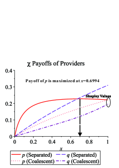
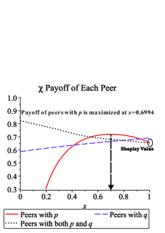
Figure 10: Example 1: $\chi$ Payoffs of Two Providers and Peers for Convex Cost Functions with $w_{p}=0.1$ and $w_{q}=3$.

Adopting non-identical weights $w_{p}=0.1$ and $w_{q}=3$, we revisit Example 1. Unlike Fig. 8 where provider $q$ monopolizes all peers because $\widetilde{\chi}_{q}^{\{q\}}(1)$ and $\widetilde{\chi}_{i}^{\{q\}}(1)$ for $i\in H$ is the biggest possible payoffs for $q$ and any peers, the monopoly for this set of weights is broken as shown in Fig. 10. Now providers $p$ and $q$ will possess $0.6994$ and $0.3006$ fraction of peers, respectively. It is remarkable that the $\chi$ payoffs are still surplus-sharing as in Figs. 8 and 9.

VI-E Stability of Coalition Structures

The $\chi$ value of the game in Example 3 with equal weights $w_{i}=1$, for all $i\in N$, is shown in Table I. As discussed in [12], NP is not suitable for a value reflecting outside options. For example, let us consider the partition $\{p_{1}p_{2},n_{1},n_{2}\}$. For the case of the A-D value, payoffs of both providers $p_{1}$ and $p_{2}$ are $0$. However, as we observe from Example 3, the best $p_{1}$ can do is to ally with $n_{1}$ to reduce her operational cost by $v(\{p_{1},n_{1}\})=5$ whereas the best $p_{2}$ can do to reduce hers by $v(\{p_{2},n_{1},n_{2}\})=9$. In other words, $p_{1}$ should release $p_{2}$ so that $p_{2}$ can create her worth because $p_{2}$ has a worthier outside option, to reflect which, $\chi$ value implementation “punishes” $p_{1}$ by giving her a negative payoff $\chi_{p_{1}}=-1$.

We also observe from Table I that players who can be better off by leaving the current coalition are paid more than others. For example, consider the partition $\{p_{1}n_{2},p_{2},n_{1}\}$. For the case of A-D payoffs, $p_{1}$ and $n_{2}$ received the same payoff $2$ (See Table 1 in [20]). However, in Table I, $n_{2}$ is paid more than $p_{1}$ because $n_{2}$ has the potential for creating the worthiest coalition $p_{1}p_{2}n_{1}n_{2}$ or $p_{2}n_{1}n_{2}$, i.e., $v(\cdot)=9$. Though $n_{2}$ will not be able to break the partition $\{p_{1}n_{2},p_{2},n_{1}\}$ according to the stability defined in Definition 3, $n_{2}$ is paid more than $p_{1}$ essentially for its assessed potential. In this case, the final form of coalition structure after its endogenous evolution is the state $\{p_{1}n_{2},p_{2}n_{1}\}$. There are now two absorbing states $\{p_{1}n_{1},p_{2},n_{2}\}$ and $\{p_{1}n_{2},p_{2}n_{1}\}$, as shown in Table I, which are stable in the sense of Definition 3. On the contrary, there does not exist any stable state for the case of A-D payoff as shown in Fig. 6 (See also Section V-B and Table 1 in [20]).

A more general result [12, Theorem 6.1] is that, if we adopt $\chi$ value to distribute the profit of the peer-assisted services, the system always has at least one stable coalition structure, irrespective of the number of providers. It it also remarkable that the following theorem holds without any restriction on operational cost $\widetilde{\Omega}_{p}(\cdot)$, whereas we assumed that $\widetilde{\Omega}_{p}(\cdot)$ is non-increasing in Section III.

Theorem 6 (Stability of $\chi$ Payoff).

For $\chi$ value, there always exists a stable coalition structure $\mathcal{P}$.

Also, it follows from [12, Corollary 6.4] that the instability of the grand coalition cannot be improved:

Corollary 3 (Stability of Grand Coalition Preserved).

The grand coalition of $\chi$ value is stable if and only if the Shapley value lies in the core.

To summarize, even if we adopt $\chi$ value, the instability of the grand coalition for the Shapley payoff which we observed in Theorem 2 remains unchanged. However, it is guaranteed that there exists a stable coalition structure for $\chi$ value.

VII Application to Delay-Tolerant Networks

In this section, we present a concrete example of the peer-assisted services in delay-tolerant networks where mobile users share certain contents with each other in a peer-to-peer fashion [22]: whenever two mobile users meet, a user whose content is more recent pushes it to the other whose content is outdated. We consider here a single class case, using the method in [22].

We assume that there exist two providers, $p$ and $q$, whose contents differ. Users who are subscribing to the content of a provider are assumed to assist the provider in any case. The fraction of users subscribing to each provider is denoted by $x_{p}^{0}$ and $x_{q}^{0}$. As discussed in Section III-A, we also assume that a non-subscribing user is allowed to assist at most one provider. Suppose that the content providers $p$ and $q$ push content updates to users, who are assisting providers, with the rate $\mu_{p}$ and $\mu_{q}$, respectively, and every user meets other users with the aggregate rate $\lambda$.

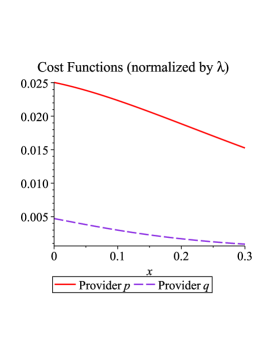
Figure 11: Cost Functions of Two Providers in the Delay-Tolerant Network.

Then it follows from the analysis in [22, Section 5.1] that, if $x_{p}\geq x_{p}^{0}$ fraction of users are assisting provider $p$, for a user who is subscribing to provider $p$, the expected age of the content and the outage probability that the age is larger than $G_{p}^{\rm max}$ are:

$$\bar{G}_{p}=\frac{1}{x_{p}\lambda}\ln\frac{x_{p}\lambda+\mu_{p}}{\mu_{p}},\quad P_{p}^{C}=\frac{{x_{p}\lambda+\mu_{p}}}{{x_{p}\lambda}+{\mu_{p}}{\rm e}^{(\mu_{p}+x_{p}\lambda)G_{p}^{\rm max}}}.$$

The above two expressions can be easily derived by using integration by parts. A provider may guarantee subscribers a certain level of quality of service by imposing constraints such as (i) $\bar{G}_{p}\leq 1\textrm{min}$ or (ii) $P_{p}^{C}\leq 0.01$ for $G_{p}^{\rm max}=10\textrm{min}$, of which we use the former here.

For instance, the cost function of provider $p$ can be computed by solving the following optimization problem over $\mu_{p}$:

$$\textstyle\min_{\mu_{p}}x_{p}\mu_{p}\quad\textrm{subject to}:~{}\bar{G}_{p}\leq g_{p}$$

where $x_{p}\mu_{p}$ corresponds to the average cost per user. The solution of this problem yields provider $p$’s cost function:

$${\widetilde{\Omega}}_{p}(x)\mathrel{:=}x\mu_{p}^{*}=\frac{x^{2}\lambda}{\exp\left(x\lambda g_{p}\right)-1}$$

where we dropped the subscript $p$ from $x_{p}$. Suppose $x_{p}^{0}=0.4$ and $x_{q}^{0}=0.3$. If providers $p$ and $q$ use $g_{p}=5/{\lambda}$ and $g_{q}=10/{\lambda}$, i.e., provider $p$ has decided to maintain a lower average age of the content than that of provider $q$, we get the cost functions ${\widetilde{\Omega}}_{p}(x+x_{p}^{0})/\lambda$ and ${\widetilde{\Omega}}_{q}(x+x_{q}^{0})/\lambda$ as shown in Fig. 11. By computing the equations in (FluidAD2) and (FluidChi), it is not difficult to see that provider $p$ monopolizes the remaining fraction of users, $1-x_{p}^{0}-x_{q}^{0}=0.3$, whether we adopt the A-D payoff or $\chi$ payoff. Nonetheless, users can receive more under the $\chi$ payoff than under the A-D payoff due to the surplus-sharing property discussed in Section VI-C.

VIII Concluding Remarks and Future Work

A quote from an interview of BBC iPlayer with CNET UK [23]: “Some people didn’t like their upload bandwidth being used. It was clearly a concern for us, and we want to make sure that everyone is happy, unequivocally, using iPlayer.”

In this paper, we have first studied the incentive structure in peer-assisted services with multiple providers, where the popular Shapley value based scheme might be in conflict with the pursuit of profits by rational content providers and peers. The key messages from our analysis are summarized as: First, even though it is fair to pay peers more because they become relatively more useful as the number of peer-assisted services increases, the content providers will not admit that peers should receive their fair shares. The providers tend to persist in single-provider coalitions. In the sense of the classical stability notion, called ‘core’, the cooperation would have been broken even if we had begun with the grand coalition as the initial condition. Second, we have illustrated yet another problems when we use the Shapley-like incentive for the exclusive single-provider coalitions. These results suggest that the profit-sharing system, Shapley value, and hence its fairness axioms, are not compatible with the selfishness of the content providers. We have proposed an alternate, realistic incentive structure in peer-assisted services, called $\chi$ value, which reflects a trade-off between fairness and rationality of individuals. Moreover, the weights of $\chi$ value can serve as a flexible knob to enable providers to bargain with peers over the dividend rate at the same time as a preventive measure to avoid cutthroat or unfair competition between providers. However, we recognize the limitation of these results, which are based on the assumption that there is no additional cost reduction other than that achieved from the peer-partition optimization. We surmise that providers in cooperation can make further expenses cut by pooling and optimizing their resources, and traffic engineering, which will transform their cost functions. The question remains open how the ramifications of this type of cooperation can be quantified in peer-assisted services.

Appendix A Appendix

A-A Proof of Theorem 1

Recall that we use notation $\widetilde{\varphi}^{{\bar{Z}}}(x)$ to denote $\widetilde{\varphi}({\bar{Z}}\cup\bar{H},v)$. We use the mathematical induction to prove this theorem. The equation (FluidAD1) holds for $|{\bar{Z}}|=0$ and ${\bar{Z}}=\emptyset$ (empty set) because we have from (FluidAD1) that there is no provider to pay and $\widetilde{\varphi}_{n}^{\emptyset}(x)=0$ for $n\in\bar{H}$.

Now we assume that (FluidAD1) holds for all $\Xi\subsetneq{\bar{Z}}$ such that $|\Xi|\leq\xi$ where $\xi\geq 0$. To prove Theorem 1, it suffices to show that (FluidAD1) also holds for all $\Xi^{\prime}\subseteq{\bar{Z}}$ such that $|\Xi^{\prime}|=\xi+1$. To this end, we first apply Axiom CE. As $\eta$ tends to infinity while $x$ remains unchanged, for $p\in\Xi^{\prime}$ and $n\in\bar{H}$, Axiom CE for the partition $\{\Xi^{\prime}\cup\bar{H}\}$ can be rewritten as follows:

$$\textstyle\sum_{p\in\Xi^{\prime}}\widetilde{\varphi}_{p}^{\Xi^{\prime}}(x)+x\widetilde{\varphi}_{n}^{\Xi^{\prime}}(x)=\sum_{p\in\Xi^{\prime}}{\widetilde{\Omega}}_{p}(0)-M_{\Omega}^{\Xi^{\prime}}(x)$$ (9)

which is the normalized (which we did in (4)) total coalition worth created by the coalition $\Xi^{\prime}\cup\bar{H}$. Another axiom we apply is Axiom FAIR (fairness) which was used by Myerson [24] to characterize the Shapley value. It follows from FAIR that

$$\textstyle\widetilde{\varphi}_{n}^{\Xi^{\prime}}(x)-\widetilde{\varphi}_{n}^{\Xi^{\prime}\setminus\{p\}}(x)=\frac{\mathrm{d}}{\mathrm{d}x}\widetilde{\varphi}_{p}^{\Xi^{\prime}}(x),\quad\mbox{for all }p\in\Xi^{\prime}.$$ (10)

Summing up (10) for all $p\in\Xi^{\prime}$ and dividing the sum by $|\Xi^{\prime}|=\xi+1$, we obtain

$$\widetilde{\varphi}_{n}^{\Xi^{\prime}}(x) \textstyle=\frac{1}{\xi+1}\sum_{p\in\Xi^{\prime}}\left(\widetilde{\varphi}_{n}^{\Xi^{\prime}\setminus\{p\}}(x)+\frac{\mathrm{d}}{\mathrm{d}x}\widetilde{\varphi}_{p}^{\Xi^{\prime}}(x)\right)$$

$$\textstyle=\frac{1}{\xi+1}\sum_{p\in\Xi^{\prime}}\widetilde{\varphi}_{n}^{\Xi^{\prime}\setminus\{p\}}(x)+\frac{1}{\xi+1}\frac{\mathrm{d}}{\mathrm{d}x}\sum_{p\in\Xi^{\prime}}\widetilde{\varphi}_{p}^{\Xi^{\prime}}(x).$$ (11)

Plugging (11) into (9), we obtain

$$\textstyle(\xi+1)\sum_{p\in\Xi^{\prime}}\widetilde{\varphi}_{p}^{\Xi^{\prime}}(x)+{x}\frac{\mathrm{d}}{\mathrm{d}x}\sum_{p\in\Xi^{\prime}}\widetilde{\varphi}_{p}^{\Xi^{\prime}}(x)$$

$$= \textstyle(\xi+1)\left(\sum_{p\in\Xi^{\prime}}{\widetilde{\Omega}}_{p}(0)-M_{\Omega}^{\Xi^{\prime}}(x)\right)-{x}\sum_{p\in\Xi^{\prime}}\widetilde{\varphi}_{n}^{\Xi^{\prime}\setminus\{p\}}(x).$$ (12)

Since we know the form of $\widetilde{\varphi}_{n}^{\Xi^{\prime}\setminus\{p\}}(x)$ for all $p\in\Xi^{\prime}$ from the assumption ($\because|\Xi^{\prime}\setminus\{p\}|=\xi$), (12) is an ordinary differential equation of the function $\sum_{p\in\Xi^{\prime}}\widetilde{\varphi}_{p}^{\Xi^{\prime}}(x)$. Denote the RHS of (12) by $G(x)$. Appealing to [4, Lemma 3], we get

$$\textstyle\sum_{p\in\Xi^{\prime}}\widetilde{\varphi}_{p}^{\Xi^{\prime}}(x)=\int_{0}^{1}u^{\xi}G(ux)\mathrm{d}u$$

$$\textstyle=\sum_{p\in\Xi^{\prime}}{\widetilde{\Omega}}_{p}(0)-\int_{0}^{1}u^{\xi}(\xi+1)M_{\Omega}^{\Xi^{\prime}}(ux)\mathrm{d}u$$

$$\textstyle-\int_{0}^{1}u^{\xi+1}{x}\sum_{p\in\Xi^{\prime}}\widetilde{\varphi}_{n}^{\Xi^{\prime}\setminus\{p\}}(ux)\mathrm{d}u,$$

$$\textstyle\frac{\mathrm{d}}{\mathrm{d}x}\sum_{p\in\Xi^{\prime}}\widetilde{\varphi}_{p}^{\Xi^{\prime}}(x)=-(\xi+1)\int_{0}^{1}u^{\xi+1}\frac{\mathrm{d}M_{\Omega}^{\Xi^{\prime}}}{\mathrm{d}x}(ux)\mathrm{d}u$$

$$\textstyle-\int_{0}^{1}u^{\xi+1}\sum_{p\in\Xi^{\prime}}\widetilde{\varphi}_{n}^{\Xi^{\prime}\setminus\{p\}}(ux)\mathrm{d}u$$

$$\textstyle-\int_{0}^{1}u^{\xi+2}{x}\sum_{p\in\Xi^{\prime}}\frac{\mathrm{d}\widetilde{\varphi}_{n}^{\Xi^{\prime}\setminus\{p\}}}{\mathrm{d}x}(ux)\mathrm{d}u$$ (13)

$$\textstyle=-(\xi+1)\int_{0}^{1}u^{\xi+1}\frac{\mathrm{d}M_{\Omega}^{\Xi^{\prime}}}{\mathrm{d}x}(ux)\mathrm{d}u$$

$$\textstyle+(\xi+1)\int_{0}^{1}u^{\xi+1}\sum_{p\in\Xi^{\prime}}\widetilde{\varphi}_{n}^{\Xi^{\prime}\setminus\{p\}}(ux)\mathrm{d}u-\sum_{p\in\Xi^{\prime}}\widetilde{\varphi}_{n}^{\Xi^{\prime}\setminus\{p\}}.$$ (14)

where the last expression follows by integrating the last term of (13) by parts. From (11) and (14), $\widetilde{\varphi}_{n}^{\Xi^{\prime}}(x)$ is rearranged as

$$\widetilde{\varphi}_{n}^{\Xi^{\prime}}(x) \textstyle=-\int_{0}^{1}u^{\xi+1}\frac{\mathrm{d}M_{\Omega}^{\Xi^{\prime}}}{\mathrm{d}x}(ux)\mathrm{d}u$$

$$\textstyle+\int_{0}^{1}u^{\xi+1}\sum_{p\in\Xi^{\prime}}\widetilde{\varphi}_{n}^{\Xi^{\prime}\setminus\{p\}}(ux)\mathrm{d}u.$$ (15)

From the assumption, $\widetilde{\varphi}_{n}^{\Xi^{\prime}\setminus\{p\}}(x)$ is given by (FluidAD1) for ${\bar{Z}}=\Xi^{\prime}\setminus\{p\}$, which is plugged into the last term of (15) to yield

$$\textstyle\int_{0}^{1}u^{\xi+1}\sum_{p\in\Xi^{\prime}}\widetilde{\varphi}_{n}^{\Xi^{\prime}\setminus\{p\}}(ux)\mathrm{d}u$$

$$\textstyle=\!-\!\displaystyle\sum_{p\in\Xi^{\prime}}\sum_{S\subseteq\Xi^{\prime}\setminus\{p\}}\textstyle\int_{0}^{1}\!\int_{0}^{1}(ut)^{|S|}(u-ut)^{\xi-|S|}\frac{\mathrm{d}M_{\Omega}^{S}}{\mathrm{d}x}(utx)u\mathrm{d}t\mathrm{d}u.$$ (16)

To reduce the double integral of (16), we use the following fact:

$$\textstyle\int_{0}^{1}\int_{0}^{1}(ut)^{|S|}(u-ut)^{\xi-|S|}f(utx)u\mathrm{d}t\mathrm{d}u$$

$$\textstyle=\int_{0}^{1}\int_{0}^{u}\tau^{|S|}(u-\tau)^{\xi-|S|}f(\tau x)\mathrm{d}\tau\mathrm{d}u$$

$$\textstyle=\int_{0}^{1}\int_{\tau}^{1}\tau^{|S|}(u-\tau)^{\xi-|S|}f(\tau x)\mathrm{d}u\mathrm{d}\tau$$

$$\textstyle=\int_{0}^{1}\frac{1}{\xi+1-|S|}\tau^{|S|}(1-\tau)^{\xi+1-|S|}f(\tau x)\mathrm{d}\tau$$ (17)

where we used the change of variable $ut=\tau$ and changed the order of the double integration with respect to $u$ and $\tau$. Plugging (17) into (16) yields

$$\textstyle\int_{0}^{1}u^{\xi+1}\sum_{p\in\Xi^{\prime}}\widetilde{\varphi}_{n}^{\Xi^{\prime}\setminus\{p\}}(ux)\mathrm{d}u$$

$$=-\sum_{p\in\Xi^{\prime}}\sum_{S\subseteq\Xi^{\prime}\setminus\{p\}}\textstyle\frac{1}{\xi+1-|S|}\int_{0}^{1}\scriptstyle u^{|S|}(1-u)^{\xi+1-|S|}\textstyle\frac{\mathrm{d}M_{\Omega}^{S}}{\mathrm{d}x}(ux)\mathrm{d}u$$

$$\textstyle=-\sum_{S\subseteq\Xi^{\prime},S\neq\Xi^{\prime}}\textstyle\int_{0}^{1}u^{|S|}(1-u)^{\xi+1-|S|}\frac{\mathrm{d}M_{\Omega}^{S}}{\mathrm{d}x}(ux)\mathrm{d}u.$$ (18)

where the last equality holds because

$$\textstyle\sum_{p\in\Xi^{\prime}}\sum_{S\subseteq\Xi^{\prime}\setminus\{p\}}f(S):\sum_{S\subseteq\Xi^{\prime},S\neq\Xi^{\prime}}f(S)$$

$$\textstyle=(\xi+1)\cdot\binom{\xi}{|S|}:\binom{\xi+1}{|S|}=\xi+1-|S|:1.$$

Plugging (18) into (15) establishes the following desired result:

$$\textstyle\widetilde{\varphi}_{n}^{\Xi^{\prime}}(x)=-\sum_{S\subseteq\Xi^{\prime}}\int_{0}^{1}u^{|S|}(1-u)^{\xi+1-|S|}\frac{\mathrm{d}M_{\Omega}^{S}}{\mathrm{d}x}(ux)\mathrm{d}u$$ (19)

from which it follows

$$\textstyle\widetilde{\varphi}_{n}^{\Xi^{\prime}}(x)-\widetilde{\varphi}_{n}^{\Xi^{\prime}\setminus\{p\}}(x)=$$

$$\textstyle-\sum_{S\subseteq\Xi^{\prime}}\int_{0}^{1}u^{|S|}(1-u)^{\xi+1-|S|}\frac{\mathrm{d}M_{\Omega}^{S}}{\mathrm{d}x}(ux)\mathrm{d}u$$

$$\textstyle+\sum_{S\subseteq\Xi^{\prime}\setminus\{p\}}\int_{0}^{1}u^{|S|}(1-u)^{\xi-|S|}\frac{\mathrm{d}M_{\Omega}^{S}}{\mathrm{d}x}(ux)\mathrm{d}u.$$

The first term of the RHS can be decomposed into the following:

$$\textstyle-\sum_{S\subseteq\Xi^{\prime}\setminus\{p\}}\int_{0}^{1}u^{|S|+1}(1-u)^{\xi+1-(|S|+1)}\frac{\mathrm{d}M_{\Omega}^{S\cup\{p\}}}{\mathrm{d}x}(ux)\mathrm{d}u$$

$$\textstyle-\sum_{S\subseteq\Xi^{\prime}\setminus\{p\}}\int_{0}^{1}u^{|S|}(1-u)^{\xi+1-|S|}\frac{\mathrm{d}M_{\Omega}^{S}}{\mathrm{d}x}(ux)\mathrm{d}u.$$

Thus, we can obtain

$$\textstyle\widetilde{\varphi}_{n}^{\Xi^{\prime}}(x)-\widetilde{\varphi}_{n}^{\Xi^{\prime}\setminus\{p\}}(x)=$$

$$\textstyle\!-\!\displaystyle\sum_{S\subseteq\Xi^{\prime}\setminus\{p\}}\textstyle\int_{0}^{1}\scriptstyle u^{|S|+1}(1-u)^{\xi-|S|}\textstyle\left(\frac{\mathrm{d}M_{\Omega}^{S\cup\{p\}}}{\mathrm{d}x}\scriptstyle(ux)\textstyle-\frac{\mathrm{d}M_{\Omega}^{S}}{\mathrm{d}x}\scriptstyle(ux)\textstyle\right)\mathrm{d}u.$$ (20)

Integrating (10) with respect to $x$ and from (20), we get

$$\textstyle\widetilde{\varphi}_{p}^{\Xi^{\prime}}(x)=$$

$$-\sum_{S\subseteq\Xi^{\prime}\setminus\{p\}}\textstyle\int_{0}^{1}\scriptstyle u^{|S|}(1-u)^{\xi-|S|}\textstyle\left[M_{\Omega}^{S\cup\{p\}}\scriptstyle(y)\textstyle-M_{\Omega}^{S}\scriptstyle(y)\textstyle\right]^{y=ux}_{y=0}\mathrm{d}u.$$

Because $M_{\Omega}^{S\cup\{p\}}(0)\textstyle-M_{\Omega}^{S}(0)={\widetilde{\Omega}}_{p}(0)$, the above equation combined with (19) finally establishes that (FluidAD1) also holds for all $\Xi^{\prime}\subseteq{\bar{Z}}$ where $|\Xi^{\prime}|=\xi+1$, hence completing the proof.

A-B Proof of Theorem 2

To prove the theorem, we need to show that the condition for the core in Definition 1 is violated, implying that it suffices to show the following:

$$\textstyle\widetilde{\varphi}_{p}^{Z}(1) \textstyle>\displaystyle\sum_{i\in{Z}}\textstyle{\widetilde{\Omega}}_{i}(0)\!-\!M_{\Omega}^{Z}(1)\!-\!\left(\!\displaystyle\sum_{i\in{Z}\setminus\{p\}}\textstyle{\widetilde{\Omega}}_{i}(0)-M_{\Omega}^{{Z}\setminus\{p\}}(1)\!\right)$$

$$\textstyle={\widetilde{\Omega}}_{p}(0)-\left(M_{\Omega}^{Z}(1)-M_{\Omega}^{{Z}\setminus\{p\}}(1)\right).$$ (21)

This means that the payoff of $p\in{Z}$ is greater than the marginal increase of the limit worth, i.e.,

$$\textstyle\lim_{\eta\to\infty}\frac{1}{\eta}v({Z}\cup H)-\lim_{\eta\to\infty}\frac{1}{\eta}v(({Z}\setminus\{p\})\cup H).$$

Subtracting the RHS of (21) from the LHS of (21) and using the expression of $\widetilde{\varphi}_{p}^{Z}(1)$ in (FluidAD1), we have

$$\textstyle M_{\Omega}^{Z}(1)-M_{\Omega}^{{Z}\setminus\{p\}}(1)$$

$$\textstyle-\displaystyle\sum_{S\subseteq{Z}\setminus\{p\}}\textstyle\int_{0}^{1}u^{|S|}(1-u)^{|{Z}|-1-|S|}\left(M_{\Omega}^{S\cup\{p\}}\scriptstyle(u)\textstyle-M_{\Omega}^{S}\scriptstyle(u)\textstyle\right)\mathrm{d}u.$$ (22)

We see from Definition 6 that $M_{\Omega}^{Z}(1)-M_{\Omega}^{{Z}\setminus\{p\}}(1)={\widetilde{\Omega}}_{p}(0)$. From the assumption, there exists a noncontributing provider which we denote by $p$. To show that (22) is strictly positive, we rewrite the last factor of the integrand as follows:

$$\textstyle M_{\Omega}^{S\cup\{p\}}(y)-M_{\Omega}^{S}(y)=$$

$$\textstyle\min\left\{\sum_{i\in S\cup\{p\}}{\widetilde{\Omega}}_{i}(y_{i})~{}\big{|}~{}\sum_{i\in S\cup\{p\}}y_{i}\leq y,y_{i}\geq 0\right\}$$

$$\textstyle-\min\left\{\sum_{i\in S}{\widetilde{\Omega}}_{i}(y_{i})~{}\big{|}~{}\sum_{i\in S}y_{i}\leq y,y_{i}\geq 0\right\}$$

where the first term in the RHS can be rearranged as

$$\textstyle\min\left\{\sum_{i\in S\cup\{p\}}{\widetilde{\Omega}}_{i}(y_{i})~{}\big{|}~{}\sum_{i\in S\cup\{p\}}y_{i}\leq y,y_{i}\geq 0\right\}$$

$$\textstyle\leq{\widetilde{\Omega}}_{p}(0)+\min\left\{\sum_{i\in S}{\widetilde{\Omega}}_{i}(y_{i})~{}\big{|}~{}\sum_{i\in S}y_{i}\leq y,y_{i}\geq 0\right\}$$

where the inequality holds from that ${\widetilde{\Omega}}_{i}(y)$, $i\in{Z}$, are non-increasing. It can be easily seen that the inequality holds by considering two cases $y_{p}=0$ and $y_{p}>0$. The inequality becomes strict when $S=\emptyset$ over some interval in $[0,x]$ whose length is positive due to the assumption that ${\widetilde{\Omega}}_{p}(y)$ is not constant in the interval $y\in[0,x]$ and non-increasing. From this, we see that (22) is greater than

$${\widetilde{\Omega}}_{p}(0)-\sum_{S\subseteq{Z}\setminus\{p\}}\int_{0}^{1}u^{|S|}(1-u)^{|{Z}|-1-|S|}{\widetilde{\Omega}}_{p}(0)\mathrm{d}u=0$$

which establishes (21), hence completing the proof.

A-C Proof of Theorem 3

To prove Theorem 3, it suffices to show that the following is positive for $\{p\}\subsetneq T$ such that $T\subseteq{Z}$:

$$\textstyle\varphi_{p}^{\{p\}}(x)-\varphi_{p}^{T}(x)=-\int_{0}^{1}M_{\Omega}^{\{p\}}\scriptstyle(ux)\textstyle\mathrm{d}u$$

$$\displaystyle\sum_{S\subseteq T\setminus\{p\}}\textstyle\int_{0}^{1}u^{|S|}(1-u)^{|T|-1-|S|}\left(M_{\Omega}^{S\cup\{p\}}\scriptstyle(ux)\textstyle-M_{\Omega}^{S}\scriptstyle(ux)\textstyle\right)\mathrm{d}u$$ (23)

which implies that the payoff of $p$ when it is the only provider of the coalition is larger than that with other providers $T\setminus\{p\}$. To this end, we first observe that, for $y\leq x$,

$$\textstyle M_{\Omega}^{S\cup\{p\}}(y)-M_{\Omega}^{S}(y)=$$

$$\textstyle\min\left\{\sum_{i\in S\cup\{p\}}{\widetilde{\Omega}}_{i}(y_{i})~{}\big{|}~{}\sum_{i\in S\cup\{p\}}y_{i}\leq y,y_{i}\geq 0\right\}$$

$$\textstyle-\min\left\{\sum_{i\in S}{\widetilde{\Omega}}_{i}(y_{i})~{}\big{|}~{}\sum_{i\in S}y_{i}\leq y,y_{i}\geq 0\right\}.$$

Here the first term in the RHS can be rearranged as

$$\textstyle\min\left\{\sum_{i\in S\cup\{p\}}{\widetilde{\Omega}}_{i}(y_{i})~{}\big{|}~{}\sum_{i\in S\cup\{p\}}y_{i}\leq y,y_{i}\geq 0\right\}$$

$$\textstyle\geq M_{\Omega}^{\{p\}}(y)+\min\left\{\sum_{i\in S}{\widetilde{\Omega}}_{i}(y_{i})~{}\big{|}~{}\sum_{i\in S}y_{i}\leq y,y_{i}\geq 0\right\}$$

where the inequality holds from that $M_{\Omega}^{\{i\}}(y)$, $i\in T$, are non-increasing. It can be easily seen that the inequality holds by considering two cases $y_{p}=0$ and $y_{p}>0$. The inequality becomes strict when $S=\emptyset$ over some interval in $[0,x]$ whose length is positive due to the assumption that ${\widetilde{\Omega}}_{p}(y)$ is not constant in the interval $y\in[0,x]$ and non-increasing. From this inequality, we have $M_{\Omega}^{S\cup\{p\}}(y)-M_{\Omega}^{S}(y)\geq M_{\Omega}^{\{p\}}(y)$ and the inequality is strict over some interval of positive length. Plugging this relation into (23) yields $\varphi_{p}^{\{p\}}(x)-\varphi_{p}^{T}(x)>0$.

Note that from (9), we have:

$$\textstyle\lim_{\eta\to\infty}v(\{p\}\cup\bar{H})/\eta\textstyle={\widetilde{\Omega}}_{p}(0)-M_{\Omega}^{\{p\}}(x)$$

$$\textstyle\leq\sum_{i\in T}{\widetilde{\Omega}}_{i}(0)-M_{\Omega}^{T}(x)=\lim_{\eta\to\infty}v(T\cup\bar{H})/\eta$$

which, when combined with $\varphi_{p}^{\{p\}}(x)>\varphi_{p}^{T}(x)$, implies the second part of the theorem.

Jeong-woo Cho received his B.S., M.S., and Ph.D. degrees in Electrical Engineering and Computer Science from KAIST, Daejeon, South Korea, in 2000, 2002, and 2005, respectively. From September 2005 to July 2007, he was with the Telecommunication R&D Center, Samsung Electronics, South Korea, as a Senior Engineer. From August 2007 to August 2010, he held postdoc positions in the School of Computer and Communication Sciences, École Polytechnique Fédérale de Lausanne (EPFL), Switzerland, and at the Centre for Quantifiable Quality of Service in Communication Systems, Norwegian University of Science and Technology (NTNU), Trondheim, Norway. He is now an assistant professor in the School of Information and Communication Technology at KTH Royal Institute of Technology, Stockholm, Sweden. His current research interests include performance evaluation in various networks such as peer-to-peer network, wireless local area network, and delay-tolerant network.

Yung Yi received his B.S. and the M.S. in the School of Computer Science and Engineering from Seoul National University, South Korea in 1997 and 1999, respectively, and his Ph.D. in the Department of Electrical and Computer Engineering at the University of Texas at Austin in 2006. From 2006 to 2008, he was a post-doctoral research associate in the Department of Electrical Engineering at Princeton University. He is now an associate professor at the Department of Electrical Engineering at KAIST, South Korea. He has been serving as a TPC member at various conferences including ACM Mobihoc, Wicon, WiOpt, IEEE Infocom, ICC, Globecom, ITC, and WASA. His academic service also includes the local arrangement chair of WiOpt 2009 and CFI 2010, the networking area track chair of TENCON 2010, the publication chair of CFI 2011-2012, and the symposium chair of a green computing, networking, and communication area of ICNC 2012. He has served as a guest editor of the special issue on Green Networking and Communication Systems of IEEE Surveys and Tutorials, an associate editor of Elsevier Computer Communications Journal, and an associate editor of Journal of Communications and Networks. He has also served as the co-chair of the Green Multimedia Communication Interest Group of the IEEE Multimedia Communication Technical Committee. His current research interests include the design and analysis of computer networking and wireless systems, especially congestion control, scheduling, and interference management, with applications in wireless ad hoc networks, broadband access networks, economic aspects of communication networks, and greening of network systems.

References

- [1] V. Valancius, N. Laoutaris, L. Massoulié, C. Diot, and P. Rodriguez, “Greening the Internet with Nano Data Centers,” in Proc. ACM CoNEXT, Dec. 2009.
- [2] M. Cha, P. Rodriguez, S. Moon, and J. Crowcroft, “On next-generation telco-managed P2P TV architectures,” in Proc. USENIX IPTPS, Feb. 2008.
- [3] RNCOS, “Global IPTV market forecast to 2014,” Market Research Report, Feb. 2011.
- [4] V. Misra, S. Ioannidis, A. Chaintreau, and L. Massoulié, “Incentivizing peer-assisted services: A fluid Shapley value approach,” in Proc. ACM Sigmetrics, Jun. 2010.
- [5] H. Park, R. Ratzin, and M. van der Schaar, “Peer-to-peer networks – protocols, cooperation and competition,” Streaming Media Architectures, Techniques, and Applications: Recent Advances, IGI Global, pp. 262–294, 2011.
- [6] W. Saad, Z. Han, M. Debbah, A. Hjørungnes, and T. Başar, “Coalitional game theory for communication networks,” IEEE Signal Processing Mag., vol. 26, no. 5, pp. 77–97, 2009.
- [7] W. Saad, Z. Han, T. Başar, M. Debbah, and A. Hjørungnes, “Hedonic coalition formation for distributed task allocation among wireless agents,” accepted for publication in IEEE Trans. Mobile Comput., Oct. 2010.
- [8] S. Hart and M. Kurz, “Endogenous formation of coalitions,” Econometrica, vol. 51, pp. 1047–1064, 1983.
- [9] A. Tutic, “The Aumann-Drèze value, the Wiese value, and stability: A note,” International Game Theory Review, vol. 12, no. 2, pp. 189–195, 2010.
- [10] A. Casajus, “On the stabiilty of coalition structures,” Economics Letters, vol. 100, no. 2, pp. 271–274, 2008.
- [11] R. Aumann and L. Shapley, Values of Non-Atomic Games. Princeton University Press, 1974.
- [12] A. Casajus, “Outside options, componenet efficiency, and stability,” Games and Economic Behavior, vol. 65, pp. 49–61, 2009.
- [13] L. Shapley, A Value for n-Person Games. In H. W. Kuhn and A. W. Tucker, editors, Contribution to the Theory of Games II, vol. 28 of Annals of Mathematics Studies, Princeton University Press, 1953.
- [14] R. Aumann and J. Drèze, “Cooperative games with coalition structures,” International Journal of Game Theory, vol. 3, pp. 217–237, 1974.
- [15] B. Peleg and P. Sudhölter, Introduction to the Theory of Cooperative Games, 2nd ed. Springer-Verlag, 2007.
- [16] R. van den Brink and G. van der Laan, “Core concepts for share vectors,” Social Choice and Welfare, vol. 18, pp. 759–784, 2001.
- [17] G. Owen, Game Theory, 3rd ed. Academic Press, 1995.
- [18] E. Pinheiro, W. Weber, and L. A. Barroso, “Failure trends in a large disk drive population,” in Proc. USENIX FAST, Feb. 2007.
- [19] M. S. Bazaraa, H. D. Sherali, and C. M. Shetty, Nonlinear Programming: Theory and Algorithms, 2nd ed. John Wiley & Sons Inc., 1993.
- [20] J. Cho and Y. Yi, “On the Shapley-like payoff mechanisms in peer-assisted services with multiple content providers,” in Proc. GameNets, Apr. 2011. [Online]. Available: http://arxiv.org/abs/1012.2332/
- [21] A. Casajus and A. Tutic, Nash bargaining, Shapley threats, and outside options. Working paper, Chair of Microeconomics, University of Leipzig, Germany, 2008.
- [22] A. Chaintreau, J.-Y. Le Boudec, and N. Ristanovic, “The age of gossip: Spatial mean field regime,” in Proc. ACM Sigmetrics, Jun. 2009.
- [23] N. Lanxon, “iPlayer uncovered: What powers the BBC’s epic creation?” CNET UK, May 2009. [Online]. Available: http://crave.cnet.co.uk/software/iplayer-uncovered-what-powers-the-bbcs-epic-creation-49302215/
- [24] R. Myerson, “Graphs and cooperation in games,” Mathematics of Operstions Research, vol. 2, pp. 225–229, 1977.