Degree Fluctuations and the Convergence Time of Consensus Algorithms

Abstract

We consider a consensus algorithm in which every node in a sequence of undirected, $B$-connected graphs assigns equal weight to each of its neighbors. Under the assumption that the degree of each node is fixed (except for times when the node has no connections to other nodes), we show that consensus is achieved within a given accuracy $\epsilon$ on $n$ nodes in time ${B+}4n^{3}B{\ln}(2n/\epsilon)$. Because there is a direct relation between consensus algorithms in time-varying environments and inhomogeneous random walks, our result also translates into a general statement on such random walks. Moreover, we give a simple proof of a result of Cao, Spielman, and Morse that the worst case convergence time becomes exponentially large in the number of nodes $n$ under slight relaxation of the degree constancy assumption.

I Introduction

Consensus algorithms are a class of iterative update schemes that are commonly used as building blocks for the design of distributed control laws. Their main advantage is robustness in the presence of time-varying environments and unexpected communication link failures. Consensus algorithms have attracted significant interest in a variety of contexts such as distributed optimization [23], [20] coverage control [14], and many other contexts involving networks in which central control is absent and communication capabilities are time-varying.

While the convergence properties of consensus algorithms in time-varying environments are well understood, much less is known about the corresponding convergence times. An inspection of the classical convergence proofs ([4, 15]) leads to convergence time upper bounds that grow exponentially with the number of nodes. It is then natural to look for conditions under which the convergence time only grows polynomially, and this is the subject of this paper.

In our main result, we show that a consensus algorithm in which every node assigns equal weight to each of its neighbors in a sequence of undirected graphs has polynomial convergence time if the degree of any given node is constant in time (except possibly during the times when the node has no connections to other nodes).

I-A Model, notation, and background

In this subsection, we define our notation, the model of interest, and some background on consensus algorithms.

We will consider only undirected graphs in this paper; this will often be stated explicitly, but when unstated every graph should be understood to be undirected by default. Given a graph $G$, we will use $N_{i}(G)$ to denote the set of neighbors of node $i$. Given a sequence of graphs $G(0),G(1),\ldots,G(k-1)$, we will use the simpler notation $N_{i}(t),d_{i}(t)$ in place of $N_{i}(G(t))$, $d_{i}(G(t))$, and we will make a similar simplification for other variables of interest.

We are interested in analyzing a consensus algorithm in which a node assigns equal weight to each one of its neighbors. We consider $n$ nodes and assume that at each discrete time $t$, node $i$ stores a real number $x_{i}(t)$. We let $x(t)=(x_{1}(t),\ldots,x_{n}(t))^{T}$. For any given sequence of graphs $G(0),G(1),G(2),\ldots$, all on the node set $\{1,\ldots,n\}$, and any initial vector $x(0)$, the algorithm is described by the update equation

$$x_{i}(t+1)=\frac{1}{d_{i}(t)}\sum_{j\in N_{i}(t)}x_{j}(t),\qquad{i=1,\ldots,n,}$$ (1)

which can also be written in the form

$$x(t+1)=A(t)x(t),$$ (2)

for a suitably defined sequence of matrices $A(0),$ $A(1),\ldots,$ $A(t-1)$. The graphs $G(t)$, which appear in the above update rule through $d_{i}(t)$ and $N_{i}(t)$, correspond to information flow among the agents; the edge $(i,j)$ is present in $G(t)$ if and only if agent $i$ uses the value $x_{{j}}(t)$ of agent ${j}$ in its update at time $t$. To reflect the fact that every agent always has access to its own information, we assume that every graph $G(t)$ contains all the self-loops $(i,i)$; as a consequence, $d_{i}(t)\geq 1$ for all $i,t$. Note that we have $[A(t)]_{ij}>0$ if and only if $(i,j)$ is an edge in $G(t)$.

We will say that the graph sequence $G(t)$ is $B$-connected if, for every $k\geq 0$, the graph obtained by taking the union of the edge sets of $G(kB),G(kB+1),\ldots,G((k+1)B-1)$ is connected. It is well known ([23, 15]) that if the graph sequence is $B$-connected for some positive integer $B$, then every component of $x(t)$ converges to a common value. In this paper, we focus on the convergence rate of this process in some natural settings. To quantify the progress of the algorithm towards consensus, we will use the function $S({x})=\max_{i}x_{i}-\min_{i}x_{i}.$ For any $\epsilon>0$, a sequence of stochastic matrices $A(0),A(1),\ldots,A(k-1)$ results in $\epsilon$-consensus if

$$S({A(k-1)\cdots A(1)A(0)x(k)})\leq\epsilon S({x(0)})$$

for all initial vectors $x(0)$; alternatively, a sequence of graphs $G(0),G(1),\ldots$ achieves $\epsilon$-consensus if the sequence of matrices $A(t)$ defined by Equations (1) and (2) achieves $\epsilon$-consensus.

As mentioned previously, we will focus on graph sequences in which every graph $G(t)$ is undirected. There are a number of reasons to be especially interested in undirected graphs within the context of consensus. For example, $G(t)$ is undirected if: (i) $G(t)$ contains all the edges between agents that are physically within some distance of each other; (ii) $G(t)$ contains all the edges between agents that have line-of-sight views of each other; (iii) $G(t)$ contains the edges corresponding to pairs of agents that can send messages to each other using a protocol that relies on acknowledgments.

It is an immediate consequence of existing convergence proofs ([4], [15]) that any sequence of $Cn^{nB}{\ln}(1/\epsilon)$ undirected $B$-connected graphs, with self-loops at every node, results in $\epsilon$-consensus. Here, $C$ is a constant that does not depend on the problem parameters $n$, $B$, and $\epsilon$. We are interested in simple conditions on the graph sequence under which the undesirable $O(n^{nB})$ scaling becomes polynomial in $n$ and $B$.

I-B Our results

Our contributions are as follows. First, in Section II, we prove our main result.

Theorem 1

Consider a sequence $G(0),G(1),\ldots,G(k-1)$ of $B$-connected undirected graphs with self-loops at each node. Suppose that for each $i$ there exists some $d_{i}$ such that $d_{i}(t)\in\{1,d_{i}\}$ for all $t$ (note that $d_{i}(t)=1$ means node $i$ has no links to any other node). If the length $k$ of the graph sequence is at least ${B+}4n^{3}B{\ln}\frac{2{n}}{\epsilon}$, then $\epsilon$-consensus is achieved.

In Section III, we give an interpretation of our results in terms of Markov chains. Theorem 1 can be interpreted as providing a sufficient condition for a random walk on a time-varying graph to forget its initial distribution in polynomial time.

In Section IV, we capitalize on the Markov chain interpretation and provide a simple proof that relaxing the assumptions of Theorem 1 even slightly can lead to a convergence time which is exponential in $n$. Specifically, if we replace the assumption that each $d_{i}(t)$ is independent of $t$ with the weaker assumption that the sorted degree sequence (say, in non-increasing order) is independent of $t$ (thus allowing nodes to “swap” degrees), exponential convergence time is possible. This was proved earlier by Cao, Spielman, and Morse (although unpublished) [5] and our contribution is to provide a simple proof.

In summary: for undirected $B$-connected graphs with self-loops, unchanging degrees is a sufficient condition for polynomial time convergence, but relaxing it even slightly by allowing the nodes to “swap” degrees leads to the possibility of exponential convergence time.

I-C Previous work

There is considerable and growing literature on the convergence time of consensus algorithms. The recent paper [15] amplified the interest in consensus algorithms and spawned a vast subsequent literature, which is impossible to survey here. We only mention papers that are closest to our own work, omitting references to the literature on various aspects of consensus convergence times that we do not address here.

Worst-case upper bounds on the convergence times of consensus algorithms have been established in [8, 6, 7, 1, 2, 11]. The papers [8, 6, 7] considered a setting slightly more general than ours, and established exponential upper bounds. The papers [1, 2] addressed the convergence times of consensus algorithms in terms of spanning trees that capture the information flow between the nodes. It was observed that in several cases this approach produces tight estimates of the convergence times. We mention also [18] which derives a polynomial-time upper bound on the time and total communication complexity required by a network of robotic agents to implement various deployment and coordination schemes. Reference [11] takes a geometric approach, and considers the convergence time in a somewhat different model, involving interactions between geographically nearest neighbors. It finds that the convergence time is quite high (either singly exponential or iterated exponential, depending on the model). Random walks on undirected graphs such as considered here are special cases of reversible agreement systems considered in the related work [12] (see also [9] and [10]). Our proof techniques are heavily influenced by the classic paper [16] and share some similarities with those used in the recent work [22], which used similar ideas to bound the convergence time of some inhomogenuous Markov chains. There are also similarities with the recent work [3] on the cover time of time-varying graphs.

Our work differs from these papers in that it studies time-varying, $B$-connected graphs and establishes convergence time bounds that are polynomial in $n$ and $B$. To the best of our knowledge, polynomial bounds on the particular consensus algorithm considered in this paper had previously been derived earlier only in [16] (under the assumption that the graph is fixed, undirected, with self-loops at every node), [19] (in the case when the matrix is doubly stochastic, which in our setting corresponds to a sequence of regular graphs $G(t)$). For the special case of graphs that are connected at every time step ($B=1$), the result has been apparently discovered independently by Chazelle [13] and the authors [21]. Our added generality allows for both disconnected graphs in which the degrees are kept constant, as well as the case where nodes temporarily disconnect from the network, setting their degree to one.

II Proof of Theorem 1

As in the statement of Theorem 1, we assume that we are given a sequence of undirected $B$-connected graphs $G({0}),G(1),\ldots$, with self-loops at each node, such that $d_{i}(t)$ equals either $d_{i}$ or $1$. Observe that $d_{i}>1$ for all $i=1,\ldots,n$, since else the sequence of graphs $G(t)$ could not be $B$-connected. We will use the notation ${\cal G}$ to refer to the class of undirected graphs with self-loops at every node such that the degree of node $i$ either $1$ or $d_{i}$. Note that the definition of ${\cal G}$ depends on the values $d_{1},\ldots,d_{n}$.

Given an undirected graph $G$, we define the update matrix $A(G)$ by

$$[A(G)]_{ij}=\begin{cases}{1}/{d_{i}(G)},&\text{ if }j\in N_{i}(G),\\ 0,&\text{ {otherwise}.}\end{cases}$$

We use $A(t)$ as a shorthand for $A(G(t))$, so that Eq.  (1) can be written as

$$x(t+1)=A(t)x(t).$$ (3)

Conversely, given an update matrix $A$ of the above form, we will use $G(A)$ to denote the graph $G$ whose update matrix is $A$. We use ${\cal A}$ to denote the set of update matrices $A(G)$ associated with graphs $G\in{\cal G}$. We define ${\bf d}$ to be the vector ${\bf d}=[d_{1},d_{2},\ldots,d_{n}]^{T}$; a simple calculation shows that ${\bf d}^{T}A={\bf d}^{T}$ for all $A\in{\cal A}$. Finally, we use $D$ to denote the matrix whose $i$th diagonal element is $d_{i}$.

We begin by identifying a weighted average that is preserved by the iteration $x(t+1)=A(t)x(t)$. For any vector $y$, we let

$$\bar{y}=\frac{{\bf d}^{T}y}{{\bf d}^{T}{\bf 1}}=\frac{\sum_{i=1}^{n}d_{i}y_{i}}{\sum_{i=1}^{n}d_{i}},$$

where ${\bf 1}$ is the vector with entries equal to 1. Observe that for any $A\in{\cal A}$,

$$\overline{Ay}=\frac{{\bf d}^{T}Ay}{{\bf d}^{T}{\bf 1}}=\frac{{\bf d}^{T}y}{{\bf d}^{T}1}=\bar{y}.$$

Consequently, if $x(t)$ evolves according to Eq. (3), then $\overline{x(t)}=\overline{x(0)}$, which we will from now on denote simply by $\bar{x}$.

With these preliminaries in place, we now proceed to the main part of our analysis, which is based on the pair of Lyapunov functions

$$V(x)=x^{T}Dx=\sum_{i=1}^{n}d_{i}x_{i}^{2},~{}~{}\mbox{ and }~{}~{}V^{\prime}(x)=\sum_{i=1}^{n}d_{i}(x_{i}-\bar{x})^{2}.$$

We will adopt the more convenient notation $V(t)$ for $V(x(t))$ and similarly $V^{\prime}(t)$ for $V^{\prime}(x(t))$.

Our first lemma provides a convenient identity for matrices in ${\cal A}$.

Lemma 2

For any $A\in{\cal A}$ such that $G(A)$ is connected (and in particular, every node $i$ has degree $d_{i}$),

$$A^{T}DA=D-\sum_{i<j}w_{ij}({\bf e}_{i}-{\bf e}_{j})({\bf e}_{i}-{\bf e}_{j})^{T},$$

where $w_{ij}$ is the $(i,j)$-th entry of $A^{T}DA$.

Remark 3

This was proven in [24] and is a generalized version of a decomposition from [25, 19]. It may be quickly verified by checking that both sides of the equation are symmetric, have identical row sums, and whenever $i<j$, the $(i,j)$-th element of both sides is $w_{ij}$. The equality of the two sides then immediately follows.

Our next lemma quantifies the decrease of $V(\cdot)$ when a vector $x$ is multiplied by some matrix $A\in{\cal A}$ associated with a connected graph $G(A)$.

Lemma 4

Fix $x\in{\mathbf{R}}^{n}$ and let $i:\{1,\ldots,n\}\rightarrow\{1,\ldots,n\}$ be a permutation such that $x_{i[1]}\leq x_{i[2]}\leq\cdots\leq x_{i[n]}$. For any $A\in{\cal A}$ such that $G(A)$ is connected,

$$V(Ax)\leq V(x)-\frac{1}{2}\sum_{l=1}^{n-1}(x_{i[l+1]}-x_{i[l]})^{2}.$$

Proof:

We may suppose without loss of generality that $x_{1}\leq x_{2}\leq\cdots\leq x_{n}$. Using Lemma 2,

$$V(Ax)=(Ax)^{T}D(Ax)=x^{T}A^{T}DAx=V(x)-\sum_{i<j}w_{ij}(x_{i}-x_{j})^{2}.$$

From the definitions of $w_{ij},A$, and $D$, we have that

$$w_{ij}=\sum_{k\in N(i)\cap N(j)}\frac{1}{d(k)},$$

and so

$$V(Ax)=V(x)-\sum_{i<j}(x_{i}-x_{j})^{2}\sum_{k\in N(i)\cap N(j)}\frac{1}{d(k)}.$$ (4)

Observe that if $l<k$, then

$$(x_{k}-x_{l})^{2}\geq(x_{l+1}-x_{l})^{2}+(x_{l+2}-x_{l+1})^{2}+\cdots+(x_{k}-x_{k-1})^{2}$$

Applying this to each term of Eq. (4), we have that

$$V(Ax)\leq V(x)-\sum_{i=1}^{n-1}W_{i}(x_{i}-x_{i+1})^{2},$$

where

$$W_{i}=\sum_{k\leq i,~{}l\geq i+1}\sum_{~{}m\in N(k)\cap N(l)}\frac{1}{d(m)}$$ (5)

We finish the proof by arguing that $W_{i}\geq 1/2$ for all $i\leq n-1$. Indeed, by the connectivity of $G(A)$, there is some node $j$ in $\{1,\ldots,i\}$ such that $j$ is connected to a node in $\{i+1,\ldots,n\}$. Let $d^{+}$ be the number of neighbors of node $j$ in $\{i+1,\ldots,n\}$ and $d^{-}$ be the number of neighbors of node $j$ in $\{1,\ldots,i\}$; naturally, $d_{j}=d^{+}+d^{-}$ and both $d^{+},d^{-}$ are at least $1$: the former by the definition of $j$, and the latter because node $j$ has a self-loop. Observe that the contribution to $W_{i}$ in Eq. (5), by running $k$ over all the $d^{-}$ neighbors of $j$ in $\{1,\ldots,i\}$ and running $l$ over all $d^{+}$ neighbors of $j$ in $\{i+1,\ldots,n\}$, is at least

$$d^{+}d^{-}\frac{1}{d_{j}}\geq\frac{d_{j}-1}{d_{j}}\geq\frac{1}{2},$$

where the final inequality is justified because the connectivity of $G(A)$ implies that $d_{j}\geq 2$. This concludes the proof. ∎

Remark 5

We note that $V(Ax)\leq V(x)$, even if $G(A)$ is not connected; this follows by applying Eq. (4) to each connected component of $G(A)$.

Lemma 6

Suppose that $x(t)$ evolves according to Eq. (3), where $G(A(t))$ is a sequence of $B$-connected graphs from ${\cal G}$. Let $i:\{1,\ldots,n\}\rightarrow\{1,\ldots,n\}$ be a permutation such that $x_{i[1]}(kB)\leq x_{i[2]}(kB)\leq\cdots\leq x_{i[n]}(kB)$. Then,

$$V(x((k+1)B))\leq V(x(kB))-\frac{1}{2}\sum_{{l}=1}^{{n}}(x_{i[l+1]}(kB)-x_{i[l]}(kB))^{2}.$$

Proof:

It suffices to prove this under the assumption that $x_{1}(kB)<x_{2}(kB)<\cdots<x_{n}(kB)$; the general case then follows by a continuity argument. We apply the bound of Lemma 4 at each time $t=kB,\ldots,(k+1)B-1$ to each connected component of $G(t)$. This yields that

$$V((k+1)B)\leq V(kB)-\frac{1}{2}\sum_{t=kB}^{(k+1)B-1}\sum_{(q,l)\in C(t)}(x_{q}(t)-x_{l}(t))^{2}$$ (6)

Here, $C(t)$ contains all the pairs $(q,l)$ such that there is some component of $G(t)$ containing both $q$ and $l$, and $x_{{q}}(t)$ immediately follows $x_{{l}}(t)$ when the nodes in that component are ordered according to increasing values of $x$.

We then observe that for every $i=1,\ldots,n-1$ there is a first time $t$ between $kB$ and $(k+1)B-1$ when there is a link between a node in $\{1,\ldots,i\}$ and a node in $\{i+1,\ldots,n\}$. Note that because there have been no links between $\{1,\ldots,i\}$ and $\{i+1,\ldots,n\}$ from time $kB$ to time $t-1$, we have that

$$\max_{j=1,\ldots,i}x_{j}(t)\leq x_{i}(kB)<x_{i+1}(kB)\leq\min_{j=i+1,\ldots,n}x_{j}(t).$$

Moreover, at time $t$, the sum on the right-hand side of Eq. (6) will contain the term $(x_{i^{\prime}}(t)-x_{i^{\prime\prime}}(t))^{2}$ where $i^{\prime}\in{\rm arg}~{}\max_{j=1,\ldots,i}x_{j}(t)$ and $i^{\prime\prime}\in{\rm arg}~{}\min_{j=i+1,\ldots,n}x_{j}(t)$. We conclude that it is possible to associate with every $i$ some triplet $i^{\prime},i^{\prime\prime},t$ such that $t\in[kB,(k+1)B-1]$, $(i^{\prime},i^{\prime\prime})\in C(t)$ and $(x_{i}(kB)-x_{i+1}(kB))^{2}\leq(x_{i^{\prime}}(t)-x_{i^{\prime\prime}}(t))^{2}$.

To complete the proof, we argue that distinct $i$ are associated with distinct triplets $i^{\prime},i^{\prime\prime},t$. Indeed, we associate $i$ with $i^{\prime},i^{\prime\prime},t$ only if $x_{i^{\prime}}(t)=\max_{j=1,\ldots,i}x_{j}(t)$ and there have been no links between $\{1,\ldots,i\}$ and $\{i+1,\ldots,n\}$ from time $kB$ to time $t-1$. Consequently if two indices $i_{1}<i_{2}$ are associated with the same triplet, it follows that ${\rm arg}~{}\max_{j=1,\ldots,i_{1}}x_{j}(t)\cap{\rm arg}~{}\max_{j=1,\ldots,i_{2}}x_{j}(t)\neq\emptyset$ which cannot be: at time $kB$, $x_{i_{2}}(kB)\geq x_{i_{1}+1}(kB)>\max_{j=1,\ldots,i_{1}}x_{j}(kB)$ and no link between a node in $\{1,\ldots,i_{1}\}$ and a node $\{i_{1}+1,\ldots,n\}$ occured from time $kB$ to time $t-1$. ∎

The following lemma may be verified through a direct calculation.

Lemma 7

Suppose $u_{1},\ldots,u_{n}$ and $w_{1},\ldots,w_{n}$ are numbers satisfying

$$\sum_{i=1}^{n}d_{i}u_{i}=\sum_{i=1}^{n}d_{i}w_{i}.$$

Then

$$\sum_{i=1}^{n}d_{i}(u_{i}-z)^{2}-\sum_{i=1}^{n}d_{i}(w_{i}-z)^{2}$$

is a constant independent of the number $z$.

Corollary 8

Suppose $x(t)$ evolves according to Eq. (3) where $G(A(t))$ is a sequence of $B$-connected graphs from ${\cal G}$. Let $i:\{1,\ldots,n\}\rightarrow\{1,\ldots,n\}$ be a permutation such that $x_{i[1]}(kB)\leq x_{i[2]}(kB)\leq\cdots\leq x_{i[n]}(kB)$. Then,

$$V^{\prime}(x((k+1)B))\leq V^{\prime}(x(kB))-\frac{1}{2}\sum_{k=1}^{n}(x_{i[l+1]}(kB)-x_{i[l]}(kB))^{2}.$$

Proof:

Lemma 6 may be restated as

$$\sum_{i=1}^{n}d_{i}(x_{i}(kB)-0)^{2}-\sum_{i=1}^{n}d_{i}(x_{i}((k+1)B)-0)^{2}\leq\frac{1}{2}\sum_{k=1}^{n}(x_{i[l+1]}(kB)-x_{i[l]}(kB))^{2}$$

But since ${\bf d}^{T}x((k+1)B)={\bf d}^{T}x(kB)$, we can apply Lemma 7 to obtain

$$\sum_{i=1}^{n}d_{i}(x_{i}(kB)-\bar{x})^{2}-\sum_{i=1}^{n}d_{i}(x_{i}((k+1)B)-\bar{x})^{2}\leq\frac{1}{2}\sum_{k=1}^{n}(x_{i[l+1]}(kB)-x_{i[l]}(kB))^{2},$$

which is a restatement of the current corollary. ∎

Remark 9

An additional consequence of Lemma 7 is that $V^{\prime}(Ax)\leq V^{\prime}(x)$ for all $A\in{\cal A}$. Remark 5 had established this property for $V(\cdot)$ and Lemma 7 implies now the same property holds for $V^{\prime}(\cdot)$.

Lemma 10

For any $x$,

$$\frac{\sum_{l=1}^{n-1}(x_{i[l+1]}-x_{i[l]})^{2}}{V^{\prime}(x)}\geq\frac{1}{n^{2}d_{\rm max}},$$

where $d_{\rm max}$ is the largest of the degrees $d_{i}$.

Proof:

We employ a variation of an argument first used in [16]. We first argue that we can make three assumptions without loss of generality: 1) that the components of $x$ are sorted in nondecreasing order, i.e., $x_{1}\leq x_{2}\leq\cdots\leq x_{n}$; 2) $\sum_{i}d_{i}x_{i}=0$, since both the numerator and denominator on the left-hand side are invariant under the addition of a constant to each component of $x$, and in particular, $V(x)=V^{\prime}(x)$; 3) ${V^{\prime}(x)=}\sum_{i}d_{i}x_{i}^{2}=1$, since the expression on the left-hand side remains invariant under multiplication of each component of $x$ by a nonzero constant.

Let $l$ be such that $d_{l}x_{l}^{2}=\max_{i}d_{i}x_{i}^{2}$. Without loss of generality, we can assume that $x_{l}>0$; else, we replace $x$ by $-x$. The condition that $\sum_{i}d_{i}x_{i}^{2}=1$ implies that $x_{l}\geq 1/\sqrt{nd_{\rm max}}$ while the condition that $\sum_{i}d_{i}x_{i}=0$ implies $x_{1}<0$. Consequently, $x_{l}-x_{{1}}\geq 1/\sqrt{nd_{\rm max}}$.We can write this as

$$(x_{2}-x_{1})+(x_{3}-x_{2})+\cdots+(x_{l}-x_{l-1})\geq\frac{1}{\sqrt{nd_{\rm max}}}.$$

Applying the Cauchy-Schwarz inequality, we get

$$(l-1)\sum_{i=1}^{l-1}(x_{i+1}-x_{i})^{2}\geq\frac{1}{nd_{\rm max}}.$$

We then use the fact that $l-1\leq n$ to complete the proof. ∎

We can now complete the proof of Theorem 1.

Proof:

From Corollary 8 and Lemma 10, we have that for all integer $k\geq 0$,

$$V^{\prime}((k+1)B)\leq(1-\frac{1}{2n^{3}})V^{\prime}(kB).$$

Because the definition of $\epsilon$-consensus is in terms of $S(x)$ rather than $V^{\prime}(x)$, we need to relate these two quantities. On the one hand, for every $x$, we have

$$V^{\prime}({x})=\sum_{i=1}^{n}d_{i}({x_{i}}-\bar{x})^{2}\leq n\sum_{i=1}^{n}({x_{i}}-\bar{x})^{2}\leq n^{2}S^{2}({x}).$$

On the other hand, for every $x$, we have

$$V^{\prime}(x)\geq\max_{i}(x_{i}-\bar{x})^{2}\geq\frac{1}{4}(\max_{i}x_{i}-\min_{i}x_{i})^{2}=\frac{1}{4}S^{2}(x).$$

Suppose that $t\geq B+4Bn^{3}\ln({2}{n}/\epsilon)$. Then at least $\lceil 4n^{3}\ln 2n/\epsilon\rceil$ time periods of length $B$ have passed, and therefore

$$S(x(t))\leq\sqrt{4V^{\prime}(x(t))}\leq 2\Big{(}1-\frac{1}{2n^{3}}\Big{)}^{{4}n^{3}\ln(2{n}/\epsilon){(1/2)}}{\sqrt{V^{\prime}(x(0))}}\leq 2{n}e^{-\ln(2{n}/\epsilon)}S(x(0))=\epsilon S(x(0)).$$

(We have used here the inequality $(1-1/x)^{x}\leq e^{-1}$, for $x\geq 1$ as well as the fact that $V^{\prime}(\cdot)$ is nonincreasing.) ∎

III Markov chain interpretation

In this section, we give an alternative interpretation of the convergence time of a consensus algorithm in terms of inhomogeneous Markov chains; this interpretation will be used in the next section. We refer the reader to the recent monograph [17] for the requisite background on Markov chains and random walks.

We consider an inhomogeneous Markov chain whose transition probability matrix at time $k$ is $A(k)$. We fix some time $t$ and define

$$P=A(0)A(1)\cdots A(t-1).$$

This is the associated $t$-step transition probability matrix: the $(i,j)$-th entry of $P$, denoted by $p_{ij}$, is the probability that the state at time $t$ is $j$, given that the initial state is $i$. Let ${\bf p}_{i}$ be the vector whose $k$th component is $p_{ik}$; thus ${\bf p}_{i}^{T}$ is the $i$th row of $P$.

We address a question which is generic in the study of Markov chains, namely, whether the chain eventually “forgets” its initial state, i.e., whether for all $i,j$, ${\bf p}_{i}-{\bf p}_{j}$ converges to zero as $t$ increases, and if so, at what rate. We will say that the sequence of matrices $A(0),A(1),\ldots,A(t-1)$ is $\epsilon$-forgetful if for all $i,j$, we have

$$\frac{1}{2}\sum_{k}|p_{ik}-p_{jk}|\leq\epsilon.$$

The above quantity, ${\frac{1}{2}}\max_{i,j}\|{\bf p}_{i}-{\bf p}_{j}\|_{1}$ is known as the coefficient of ergodicity of the matrix $P$, and appears often in the study of consensus algorithms (see, for example, [8]). The result that follows relates the times to achieve $\epsilon$-consensus or $\epsilon$-forgetfulness, and is essentially the same as Proposition 4.5 of [17].

Proposition 11

The sequence of matrices $A(0),A(1),\ldots,$ $A(t-1)$ is $\epsilon$-forgetful if and only if the sequence of matrices $A(t-1),A(t-2),\ldots,A(0)$ results in $\epsilon$-consensus (i.e., $S(Px)\leq\epsilon S(x)$, for every vector $x$.)

Proof:

Suppose that the matrix sequence $A(0),A(1),\ldots,$ $A(t-1)$ is $\epsilon$-forgetful, i.e., that $\frac{1}{2}\sum_{k}|p_{ik}-p_{jk}|\leq\epsilon$, for all $i$ and $j$. Given a vector $x$, let $c=(\max_{k}x_{k}+\min_{k}x_{k})/2$. Note that $\|x-c{\bf 1}\|_{\infty}=(\max_{k}x_{k}-\min_{k}x_{k})/2=S(x)/2$. We then have

$$|[Px]_{i}-[Px]_{j}|=\Big{|}\sum_{k}(p_{ik}-p_{jk})(x_{k}-c)\Big{|}\leq\|{\bf p}_{i}-{\bf p}_{j}\|_{1}\cdot\|x-c{\bf 1}\|_{\infty}\leq\epsilon S(x).$$

Since this is true for every $i$ and $j$, we obtain $S(Px)\leq\epsilon S(x)$, and the sequence $A(t-1),A(t-2),\ldots,A(0)$ results in $\epsilon$-consensus.

Conversely, suppose that the sequence of matrices $A(t-1),A(t-2),\ldots,A(0)$ results in $\epsilon$-consensus. Fix some $i$ and $j$. Let $x$ be a vector whose $k$th component is $1/2$ if $p_{ik}\geq p_{jk}$ and $-1/2$ otherwise. Note that $S(x)=1$. We have

$$\frac{1}{2}\|{\bf p}_{i}-{\bf p}_{j}\|_{1}=({\bf p}_{i}^{T}-{\bf p}_{j}^{T})x=[Px]_{i}-[Px]_{j}\leq\epsilon S(x)=\epsilon,$$

where the last inequality made use of the $\epsilon$-consensus assumption. Thus, the sequence of matrices $A(0),A(1),\ldots,A(t-1)$ is $\epsilon$-forgetful. ∎

We will use Proposition 11 for the special case of Markov chains that are random walks. Given an undirected graph sequence sequence $G(0),G(1),\ldots$, we consider the random walk on the state-space $\{1,\ldots,n\}$ which, at time $t$, jumps to a uniformly chosen random neighbor of its current state in $G(t)$. We let $A(0),A(1),\ldots$ be the associated transition probability matrices. We will say that a sequence of graphs is $\epsilon$-forgetful whenever the corresponding sequence of transition probability matrices is $\epsilon$-forgetful. Proposition 11 allows us to reinterpret Theorem 1 as follows: random walks on time-varying undirected $B$-connected graphs with self-loops and degree constancy forget their initial distribution in a polynomial number of steps.

IV A counterexample

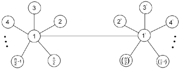
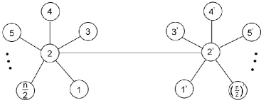
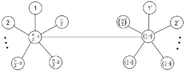
Figure 1: The top-left figure shows graph $G(0)$; top-right shows $G(1)$; bottom-left shows $G({(n/2)-2})$; bottom-right shows $G({(n/2)-1})$. As these figures illustrate, $G(t+1)$ is obtained by applying a circular shift to each half of $G(t)$. Every node has a self-loop which is not shown. For aesthetic reasons, instead of labeling the nodes as $1,\ldots,n$, we label them with $1,\ldots,n/2$ and $1^{\prime},\ldots,(n/2)^{\prime}$.

In this subsection, we show that it is impossible to relax the condition of unchanging degrees in Theorem 1. In particular, if we only impose the slightly weaker condition that the sorted degree sequence (the non-increasing list of node degrees) does not change with time, the time to achieve $\epsilon$-consensus can grow exponentially with $n$. This is an unpublished result of Cao, Spielman, and Morse [5]; we provide here a simple proof. We note that the graph sequence used in the proof (see Figure 1) is similar to the sequence used in [3] to prove an exponential lower bound on the cover time of time-varying graphs.

Proposition 12

Let $n$ be even and let $t$ be an integer multiple of $n/2$. Consider the graph sequence of length $t=kn/2$, consisting of periodic repetitions of the reversal of the length-$n/2$ sequence described in Figure 1. For this graph sequence to result in $(1/4)$-consensus, we must have $t\geq 2^{(n/2)}/{8}$.

Proof:

Suppose that this graph sequence of length $t$ results in $(1/4)$-consensus. Then Proposition 11 implies that the sequence $G^{\prime}$ of length $t$ consisting of periodic repetitions of the length $n/2$ sequence described in Figure 1 is $(1/4)$-forgetful. Let $p_{ij}$ be the associated $t$-step transition probabilities.

Let $T$ be the time that it takes for a random walk that starts at state $n/2$ at time $0$ to cross into the right-hand side of the graph, let $\delta$ be the probability that $T$ is less than or equal to $t$, and define $R$ to be the set of nodes on the right side of the graph, i.e., $R=\{1^{\prime}\ldots(n/2)^{\prime}\}$. Clearly,

$$\sum_{j^{\prime}\in R}p_{(n/2),j^{\prime}}\leq P(T\leq t)=\delta,$$

since a walk located in $R$ at time $t$ has obviously transitioned to the right-hand side of the graph by $t$. Next, symmetry yields $\sum_{j^{\prime}\in R}p_{(n/2)^{\prime},j^{\prime}}\geq 1-\delta$. Using the fact that the graph sequence is $(1/4)$-forgetful in the first inequality below, we have

$$\frac{1}{2}\geq\sum_{j^{\prime}\in R}|p_{(n/2)^{\prime},j^{\prime}}-p_{((n/2),j^{\prime}}|\geq\sum_{j^{\prime}\in R}p_{(n/2)^{\prime},j^{\prime}}-\sum_{j^{\prime}\in R}p_{(n/2),j^{\prime}}\geq(1-\delta)-\delta=1-2\delta,$$

which yields that $\delta\geq 1/4$. By viewing periods of length $t$ as a single attempt to get to the right half of the graph, with each attempt having probability at least $1/4$ to succeed, we obtain $E[T]\leq 4t$.

So far, we have not used the structure of the graphs beyond the fact that they can partitioned into a right-side and a left-side. We now make the observation which may be viewed as the motivation behind choosing this particular graph sequence. Let us say that node $i$ has emerged at time $t$ if node $i$ was the center of the left-star in $G^{\prime}(t-1)$; for example, node $1$ has emerged at time $1$, node $2$ has emerged at time $2$, and so on. By symmetry, $T$ is the expected time until a random walk starting at an emerged node crosses to the right-hand side of the graph. Observe that, starting from an emerged node, the random walk will transition to the right-hand side of the graph if it takes the self-loop $n/2-1$ consecutive times and then, once it is at the center, takes the link across; however, if it fails to take the self-loop during the first $n/2-1$ times, it then transitions to a newly emerged node. This implies that the expected time to transition to the right hand side from an emerged node is at least the expected time until the walk takes $n/2-1$ self-loops consecutively: $2^{(n/2)-1}\leq E[T]$.

Putting this together with the previous inequality $E[T]\leq 4t$, we immediately have the desired result. ∎

References

- [1] D. Angeli, P.-A. Bliman, “Tight estimates for convergence of some non-stationary consensus algorithms,” Systems and Control Letters, vol. 57, no. 12, pp. 996-1004, 2008.
- [2] D. Angeli, P.-A. Bliman, “Convergence speed of unsteady distributed consensus: decay estimate along the settling spanning-trees,” SIAM Journal on Control and Optimization, vol. 48, no. 1, pp. 1-32, 2009.
- [3] C. Avin, M. Koucky, Z. Lotker, “How to explore a fast-changing world,” Proceedings 35th International Colloquium on Automata, Languages and Programming, 2008.
- [4] D. P. Bertsekas and J. N. Tsitsiklis, Parallel and Distributed Computation: Numerical Methods, Prentice Hall, 1989.
- [5] Ming Cao, personal communication, 2006.
- [6] M. Cao, A. S. Morse, B. D. O. Anderson, “Reaching a consensus in a dynamically changing environment: a graphical approach,” SIAM Journal on Control and Optimization, vol. 47, no. 2, pp. 575-600, 2008.
- [7] M. Cao, A. S. Morse, B. D. O. Anderson, “Reaching a consensus in a dynamically changing environment: convergence rates, measurement delays, and asynchronous events,” SIAM Journal on Control and Optimization, vol. 47, no. 2, pp. 575-600, 2008.
- [8] M. Cao, D. Spielman, A. S. Morse, “A lower bound on convergence of a distributed network consensus slgorithm,” Proceedings of the 44th IEEE Conference on Decision and Control and European Control Conference, Madrid, Spain, Dec. 2005.
- [9] B. Chazelle, “Analytical tools for natural algorithms,” Proceedings of the First Symposium on Innovations in Computer Science, Beijing, China, Jan. 2010.
- [10] B. Chazelle, “The convergence of bird flocking,” Proceedings of the 26th Annual Symposium on Computational Geometry, Snowbird, USA, Jun. 2010.
- [11] B. Chazelle, “Natural algorithms,” Proceedings of the ACM-SIAM Symposium on Discrete Algorithms, New York, USA, Jan. 2009.
- [12] B. Chazelle, “‘The total s-energy of a multiagent system,” SIAM Journal on Control and Optimization, vol. 49, no. 4, pp. 1680-1706, 2011.
- [13] B. Chazelle, “The total s-energy of a multiagent system,” http://arxiv.org/abs/1004.1447, April 2010.
- [14] C. Gao, J. Cortes, F. Bullo, “Notes on averaging over acyclic graphs and discrete coverage control,” Automatica, vol. 44, no. 8, pp. 2120-2127, 2008.
- [15] A. Jadbabaie, J. Lin, and A. S. Morse, “Coordination of groups of mobile autonomous agents using nearest neighbor rules,” IEEE Transactions on Automatic Control, vol. 48, no. 3, pp. 988-1001, 2003.
- [16] H. J. Landau, A. M. Odlyzko, “Bounds for eigenvalues of certain stochastic matrices,” Linear Algebra and Its Applications, vol. 38, pp. 5-15, 1981.
- [17] D. A. Levin, Y. Peres, and E. L. Wilmer, Markov Chains and Mixing Times, American Mathematical Society, 2008.
- [18] S. Martinez, F. Bullo, J. Cortes, E. Frazzoli, “On synchronous robotic networks part II: time complexity of rendezvous and deployment algorithms,” IEEE Transactions on Automatic Control, vol. 52, no. 12,pp. 2214-2226, 2007.
- [19] A. Nedic, A. Olshevsky, A. Ozdaglar, and J. N. Tsitsiklis, “On distributed averaging algorithms and quantization effects,” IEEE Transactions on Automatic Control, vol. 54, no. 11, pp. 2506-2517, 2009.
- [20] A. Nedic, A. Ozdaglar, “Distributed subgradient methods for multi-agent optimization,” IEEE Transactions on Automatic Control, vol. 54, no. 1, pp. 48-61, 2009.
- [21] A. Olshevsky, “Degree Flucutations and Convergence Times of Consensus Algorithms,” talk delivered at Princeton University, Dec 2010, http://netfiles.uiuc.edu/aolshev2/www/princetonslides.ps.
- [22] L. Saloff-Coste, J. Zuniga, “Convergence of some time inhomogeneous Markov chains via spectral techniques,” Stochastic Processes and their Applications, vol. 117, pp. 961-979, 2007.
- [23] J. N. Tsitsiklis, D. P. Bertsekas, and M. Athans, “Distributed asynchronous deterministic and stochastic gradient optimization algorithms,” IEEE Transactions on Automatic Control, vol. 31, no. 9, 1986, pp. 803-812.
- [24] B. Touri and A. Nedic, “On existence of a quadratic comparison function for random weighted averaging dynamics and its implications,” Proceedings of the 50th IEEE Conference on Decision and Control, 2011.
- [25] L. Xiao and S. Boyd, ”Fast linear iterations for distributed averaging,” Systems and Control Letters, 53:65-78, 2004