Abstract

Accepting validity of self-consistent theory of localization by Vollhardt and W${\rm{\ddot{o}}}$lfle, we derive the finite-size scaling procedure used for studies of the critical behavior in $d$-dimensional case and based on the consideration of auxiliary quasi-1D systems. The obtained scaling functions for $d=2$ and $d=3$ are in good agreement with numerical results: it signifies the absence of essential contradictions with the Vollhardt and W${\rm{\ddot{o}}}$lfle theory on the level of raw data. The results $\nu=1.3\,-\,1.6$, usually obtained at $d=3$ for the critical exponent $\nu$ of the correlation length, are explained by the fact that dependence $L+L_{0}$ with $L_{0}>0$ ($L$ is the transversal size of the system) is interpreted as $L^{1/\nu}$ with $\nu>1$. For dimensions $d\geq 4$, the modified scaling relations are derived; it demonstrates incorrectness of the conventional treatment of data for $d=4$ and $d=5$, but establishes the constructive procedure for such a treatment. Consequences for other variants of finite-size scaling are discussed.

1. INTRODUCTION

The contemporary situation in investigation of the Anderson localization is characterized by the fact that the results of numerical modelling (see a review article [1]) contradict all other information on the critical behavior [1, 2, 3]. Such situation is unacceptable, since undermines a belief in analytical theory.

The critical behavior of conductivity $\sigma$ and the correlation length $\xi$

$$\sigma\propto\tau^{s}\,,\qquad\xi\propto|\tau|^{-\nu}$$

($\tau$ is a distance to the transition point) obtained from the self-consistent theory of localization by Vollhardt and W${\rm{\ddot{o}}}$lfle [4, 5], has a form

$$\nu=\left\{\begin{array}[]{cc}1/(d-2)\,,&\quad 2<d<4\\ 1/2\,,&\quad d>4\end{array}\right.\,,\qquad\quad s=1\,,\quad 2<d<\infty\,,$$

($d$ is the dimension of space), and in fact summarizes all known results. Indeed, the formula (2):

(a) distinguishes values $d_{c1}=2$ and $d_{c2}=4$ as the lower and upper critical dimensions, which are known from independent arguments (see [2, 6] for details);

(b) agrees with theory for $d=2+\epsilon$ [7]

$$\nu=\frac{1}{\epsilon}+0\cdot\epsilon^{0}+0\cdot\epsilon^{1}+O(\epsilon^{2})\,;$$

(c) satisfies the Wegner scaling relation $s=(d-2)\nu$ [8] for $d<d_{c2}$;

(d) gives independent of $d$ critical exponents for $d>d_{c2}$, as it is typical for the mean-field theory;

(e) agrees with the results $\nu=1/2$ [9, 10] and $s=1$ [11] for $d=\infty$;

(f) agrees with the experimental results $s\approx 1$, $\nu\approx 1$ for $d=3$, obtained by the measurement of conductivity and dielectric susceptibility [12, 13]. 

It is clear that the Vollhardt and W${\rm{\ddot{o}}}$lfle theory gives at least a very successful approximation, satisfying all general principles and reproducing all known results. More than that, a suspicion arises that the result (2) is exact [14] . This conjecture is supported by the paper [16], where Eq. 2 is derived without model approximations on the basis of symmetry analysis.

As for numerical results [17]–[31], they can be summarized by the empirical formula $\nu\approx 0.8/(d-2)+0.5$ [25], which has the evident fundamental defects. Recent developments make a situation even worse giving for $d=3$ values $\nu=1.54\pm 0.08$ [24], $\nu=1.45\pm 0.08$ [26], $\nu=1.40\pm 0.15$ [27], $\nu=1.57\pm 0.02$ [29], etc.

In our opinion, it means the existence of serious defects in the conventional numerical algorithms. It is not reasonable to call in question the raw data, which are obtained independently by many groups; but it is possible to doubt the algorithms themselves, which are not based on any serious theory. In particular, there is a possibility of rough violation of scaling [32], or existence of the large characteristic length scale [33, 3].

In the present paper, the following approach is accepted. We suppose that the Vollhardt and W${\rm{\ddot{o}}}$lfle theory (Sec. 2) is correct (there are real grounds for such assumption [16]) and derive the quantities which are immediately ”measured” in the numerical experiments. Then comparison can be made on the level of the raw data, avoiding the suspicious treatment procedure.

We restrict the discussion by the popular variant of finite-size scaling based on consideration of auxiliary quasi-1D systems [34]. Thus, instead of the infinite 3D system one consider the system of size $L\times L\times L_{z}$, where $L_{z}\to\infty$. Such system is topologically one-dimensional and does not possess the long-range order: so the corresponding correlation length $\xi_{1D}$ is finite. If $\xi_{1D}$ can be calculated, then its dependence at $L\to\infty$ allows to registrate phase transitions in the initial $3D$ system: it appears, that $\xi_{1D}/L\to\infty$ in the phase with long-range order and $\xi_{1D}/L\to 0$ in the phase with short-range correlations [34, 32]. In the numerical studies, the following scaling relation is usually postulated

$$\frac{\xi_{1D}}{L}=F\left(\frac{L}{\xi}\right)\,.$$

It is based on the assumption that the correlation length $\xi$ of the considered $d$-dimensional system is the only essential length scale, so $L$ enters only in the combination $L/\xi$. If this relation is valid, then the quantity $\xi_{1D}/L$ depends on $L$ in accordance with Fig. 1:

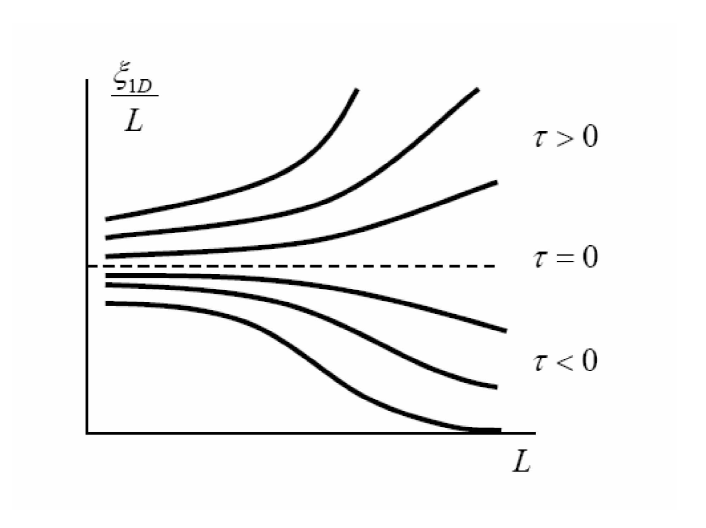
Figure 1: Dependence of the scaling parameter $\xi_{1D}/L$ on the transversal size $L$ of the system.

it remains constant at the critical point, while all curves for $\tau>0$ (and correspondingly $\tau<0$) can be reduced to one universal curve by the scale transformation. If two curves for $\tau=\tau_{1}$ and $\tau=\tau_{2}$ are calculated, then the scale transformation allows to determine the ratio of two correlation lengths. Taking succession $\tau_{1}$, $\tau_{2},\,\ldots$, one can determine $\xi(\tau_{i})$ apart from numerical factor and to investigate its critical behavior.

We demonstrate below, that the scaling relation (4) is indeed valid in the limit of large $\xi$ and $L$ for space dimensions $d<4$, while calculation of the scaling function $F$ for $d=2$ and $d=3$ shows a good agreement with numerical results (Sec. 3). It signifies that the Vollhardt and W${\rm{\ddot{o}}}$lfle theory is confirmed on the level of raw data. Section 4 clarifies why values of the exponent $\nu$ in the numerical experiments for $d=3$ are always greater than unity: in the vicinity of the critical point the scaling parameter $\xi_{1D}/L$ behaves as $\tau(L+L_{0})$ with $L_{0}>0$, which is conventionally interpreted as $\tau L^{1/\nu}$ with $\nu>1$.

For higher dimensions, the scaling relation (4) cannot be correct, and it can be stated on the level of a theorem. The problem of the Anderson transition can be exactly reduced to the $\phi^{4}$ field theory [6, 35, 36, 37], which is non-renormalizable for $d>4$ [38, 39]. Therefore, the ultraviolet cut-off (i. e. atomic scale) cannot be excluded from results, and $\xi$ is certainly not the only relevant length scale. However, it is possible to derive the modified scaling relations

$$y=F(x)$$

with

$$y=\frac{\xi_{1D}}{L}\left(\frac{a}{L}\right)^{(d-4)/3}\,,\qquad x=\frac{\xi}{L}\left(\frac{a}{L}\right)^{(d-4)/3}\,,\qquad d>4$$

and

$$y=\frac{\xi_{1D}}{L}\left[\ln(L/a)\right]^{-1/3}\,,\qquad x=\frac{\xi}{L}\,\frac{\left[\ln(L/a)\right]^{1/6}}{\left[\ln(\xi/a)\right]^{1/2}}\,,\qquad d=4,$$

demonstrating incorrectness of the conventional treatment of data for $d=4$ and $d=5$ [1], but establishing the constructive procedure for such a treatment (Sec. 5). The modified scaling (5) with

$$y=\frac{\xi_{1D}}{L}\left[\frac{\epsilon}{1-(L/a)^{-\epsilon}}\right]^{1/3}\,,\qquad x=\frac{\xi}{L}\,\frac{\left[1-(L/a)^{-\epsilon}\right]^{1/6}}{\left[(\xi/a)^{\epsilon}-1\right]^{1/2}}\,\frac{\epsilon^{1/3}}{(L/a)^{-\epsilon/2}}\,,\qquad d=4-\epsilon$$

can be derived also for $d=4-\epsilon$ dimensions. It can be used for alternative treatment at $d=3$, in order to estimate the systematic errors related with possible existence of the large length scale. Finally, in Sec. 6 we discuss some consequences of the present analysis for other variants of finite-size scaling.

2. VOLLHARDT AND W${\rm{\ddot{O}}}$LFLE THEORY

The Vollhardt and W${\rm{\ddot{o}}}$lfle theory is based on existence of the diffusion pole in the irreducible four-leg vertex $U_{{\bf k}{\bf k}^{\prime}}({\bf q})$,

$$U_{{\bf k}{\bf k}^{\prime}}({\bf q})=U_{{\bf k}{\bf k}^{\prime}}^{reg}({\bf q})+\frac{F({\bf k},{\bf k}^{\prime},{\bf q})}{-i\omega+D(\omega,{\bf k}+{\bf k}^{\prime})({\bf k}+{\bf k}^{\prime})^{2}}\,,$$

entering the Bethe–Salpiter equation and playing the role of the scattering probability $W_{{\bf k}{\bf k}^{\prime}}$ in the quantum kinetic equation. Neglecting the spatial dispersion of the diffusion coefficient  and using the estimate in the spirit of $\tau$-approximation, $D\propto\langle U\rangle^{-1}$, where $\langle...\rangle$ is averaging over momenta, we come to the self-consistency equation of the Vollhardt and W${\rm{\ddot{o}}}$lfle theory

$$D\sim\left[U_{0}+F_{0}\int\frac{d^{d}q}{-i\omega+D(\omega,q)q^{2}}\right]^{-1}\,.$$

It can be obtained by approximate solution of the Bethe–Salpiter equation [4], or by the accurate analysis of spectral properties of the quantum collision operator [16]. It can be written in the physically clear form, if coefficients are estimated for weak disorder (which is actual for lower dimensions) and a situation near the band center in the Anderson model is implied:

$$\frac{E^{2}}{W^{2}}=\frac{D}{D_{min}}+\Lambda^{2-d}\int\limits_{|q|<\Lambda}\frac{d^{d}q}{(2\pi)^{d}}\,\frac{1}{(-i\omega/D)+q^{2}}\,.$$

Here $E$ is the energy of the bandwidth order, $W$ is the amplitude of disorder, $\Lambda$ is the ultraviolet cut-off, $D_{min}$ is a characteristic scale of the diffusion coefficient corresponding to the Mott minimal conductivity. Generally, some monotonic function of $W$ is appearing in the left-hand side, but it is not essential for subsequent considerations.

Let introduce the basic integral

$$I(m)=\int\limits_{|q|<\Lambda}\frac{d^{d}q}{(2\pi)^{d}}\,\frac{1}{m^{2}+q^{2}}\,,$$

which can be estimated for $m\ll\Lambda$ as

$$I(m)=\left\{\begin{array}[]{cc}c_{d}/m^{2-d}\,,&d<2\\ c_{2}\ln(\Lambda/m)\,,&d=2\\ I(0)-c_{d}m^{d-2}\,,&2<d<4\\ I(0)-c_{4}m^{2}\ln(\Lambda/m)\,,&d=4\\ I(0)-c_{d}m^{2}\Lambda^{d-4}\,,&d>4\end{array}\right.\,,$$

where

$$c_{d}=\left\{\begin{array}[]{cc}\pi K_{d}/(2\sin(\pi d/2))\,,&d<2\\ 1/2\pi\,,&d=2\\ \pi K_{d}/|2\sin(\pi d/2)|\,,&2<d<4\\ 1/(8\pi^{2})\,,&d=4\\ K_{d}/(d-4)\,,&d>4\end{array}\right.\,,$$

and $K_{d}=\left[2^{d-1}\pi^{d/2}\Gamma(d/2)\right]^{-1}$ is the surface of the $d$-dimensional unit sphere divided by $(2\pi)^{d}$. The metallic phase is possible, when value of $I(0)$ is finite, i. e. for $d>2$. Accepting $D=const>0$ for $\omega\to 0$ and specifying $\tau$ as a distance to transition, one has

$$D=D_{min}\,\tau\,,\qquad\tau=\frac{E^{2}}{W^{2}}-I(0)\Lambda^{2-d}\,,$$

i. e. the exponent of conductivity is unity, in agreement with (2). In the dielectric phase we make substitution

$$D=-i\omega\xi^{2}\,,\qquad\xi=m^{-1}\,,$$

where $\xi$ is the correlation length. Then Eq. 11 gives

$$\xi\sim a\frac{E^{2}}{W^{2}}\,,\qquad d=1\,,$$

$$\xi\sim a\exp\left(2\pi\frac{E^{2}}{W^{2}}\right)\,,\qquad d=2\,,$$

$$\xi\sim a|\tau|^{-\nu}\,,\qquad d>2\,,$$

with the exponent $\nu$ defined by Eq. 2. In what follows, we accept $a=\Lambda^{-1}$, so $a$ is the atomic length scale, not necessary coinciding with the lattice spacing.

3. SCALING FUNCTIONS FOR $D<4$

3.1. Definition of scaling functions

For description of quasi-1D systems it is sufficient to present the basic integral (12) in the following form

$$I(m)=\frac{1}{L^{d-1}}\sum\limits_{|q_{\bot}|<\Lambda}\,\int\limits_{-\Lambda}^{\Lambda}\,\frac{dq_{||}}{2\pi}\,\frac{1}{m^{2}+q_{||}^{2}+q_{\bot}^{2}}\,,\qquad m^{-1}=\xi_{1D}$$

where $d$-dimensional vector $q=(q_{1},q_{2},\ldots,q_{d})$ is replaced by its transversal and longitudinal components

$$q_{\bot}=(q_{1},q_{2},\ldots,q_{d-1})\,,\qquad q_{||}=q_{d}\,,$$

and the first is considered as discrete, running the usual allowed values. The term with $q_{\bot}=0$ has divergency $m^{-1}$ for $m\to 0$, so the system is always localized.

After integration over $q_{||}$, the following decomposition is convenient:

$$I(m)=\frac{1}{L^{d-1}}\,\frac{1}{\pi m}\,{\rm arctg}\frac{\Lambda}{m}\,+$$

$$+\frac{1}{\pi L^{d-1}}\sum\limits_{\begin{array}[]{c}{\scriptstyle q_{\bot}\neq 0}\\ {\scriptstyle|q_{\bot}|<\Lambda}\end{array}}\left(\,\frac{1}{\sqrt{m^{2}+q_{\bot}^{2}}}\,{\rm arctg}\frac{\Lambda}{\sqrt{m^{2}+q_{\bot}^{2}}}\,-\,\frac{1}{|q_{\bot}|}\,{\rm arctg}\frac{\Lambda}{|q_{\bot}|}\right)\,+$$

$$+\,\frac{1}{\pi L^{d-1}}\sum\limits_{\begin{array}[]{c}{\scriptstyle q_{\bot}\neq 0}\\ {\scriptstyle|q_{\bot}|<\Lambda}\end{array}}\frac{1}{|q_{\bot}|}\,{\rm arctg}\frac{\Lambda}{|q_{\bot}|}\,\equiv\,I_{1}(m)+I_{2}(m)+I_{3}(0)\,.$$

We separated the term with $q_{\bot}=0$, while the remaining sum was rearranged by subtraction and addition of the analogous sum with $m=0$. In the first term one has trivially

$$I_{1}(m)=\frac{1}{L^{d-2}}\left\{\frac{1}{2mL}+O\left(\frac{a}{L}\right)\right\}\,.$$

The second term can be transformed by taking the limit $\Lambda\to\infty$ and substituting $q_{\bot}=2\pi\vec{s}/L$, where $\vec{s}=(s_{1},\ldots,s_{d-1})$ is a vector with integer components $s_{i}=0,\pm 1,\pm 2,\ldots$:

$$I_{2}(m)=\frac{1}{L^{d-2}}H_{0}(mL)+O\left(m^{2}\Lambda^{d-4}\right)\,,$$

$$H_{0}(z)=\frac{1}{4\pi}\sum\limits_{\vec{s}\neq 0}\left(\,\frac{1}{\sqrt{|\vec{s}|^{2}+(z/2\pi)^{2}}}-\,\frac{1}{|\vec{s}|}\,\right)\,.$$

The third term can be estimated at $L\to\infty$ by the replacement of summation by integration. For finite $L$ and $d>2$ it has a structure

$$I_{3}(0)=\Lambda^{d-2}\left\{b_{0}+b_{1}\left(\frac{a}{L}\right)^{d-2}+b_{2}\left(\frac{a}{L}\right)^{d-1}+\ldots\right\}\,.$$

Substituting (20–22) in the self-consistency equation (11), we have for $d>2$

$$\left(\frac{L}{a}\right)^{d-2}\left[\tau+O(m^{2}a^{2})\right]+O\left(\frac{a}{L}\right)=b_{1}+H_{0}(mL)+\frac{1}{2mL}$$

where we replaced

$$\tau=\frac{E^{2}}{W^{2}}-b_{0}$$

in agreement with definition (15), since $b_{0}$ corresponds to $I(0)$, calculated in the integral approximation. Expressing $\tau$ through the correlation length $\xi$ of the $d$-dimensional system ($\xi^{-1/\nu}\sim|\tau|=\pm\tau$) and omitting the terms dissapearing at $a\to 0$, we have

$$\pm c_{d}\left(\frac{L}{\xi}\right)^{d-2}=H\left(\frac{L}{\xi_{1D}}\right)$$

$$H(z)=b_{1}+\frac{1}{4\pi}\sum\limits_{\vec{s}\neq 0}\left(\,\frac{1}{\sqrt{|\vec{s}|^{2}+(z/2\pi)^{2}}}-\,\frac{1}{|\vec{s}|}\,\right)\,+\,\frac{1}{2z}$$

i. e. the scaling relation (4) between variables $\xi_{1D}/L$ and $\xi/L$, consisting of two branches.

For $d=2$ we have instead (22)

$$I_{3}(0)==\frac{1}{2\pi}\ln\frac{L}{a}+b_{1}+\ldots$$

and, using the result from Sec. 2

$$\frac{E^{2}}{W^{2}}=\frac{1}{2\pi}\ln\frac{\xi}{a}\,\,,$$

obtain the scaling relation in the form

$$\frac{1}{2\pi}\ln\left(\frac{\xi}{L}\right)=H\left(\frac{L}{\xi_{1D}}\right)$$

with the previous definition of $H(z)$. The functions $H(z)$ for $d=2$ and $d=3$ are presented in Fig. 2, where $b_{1}=0$ was accepted.

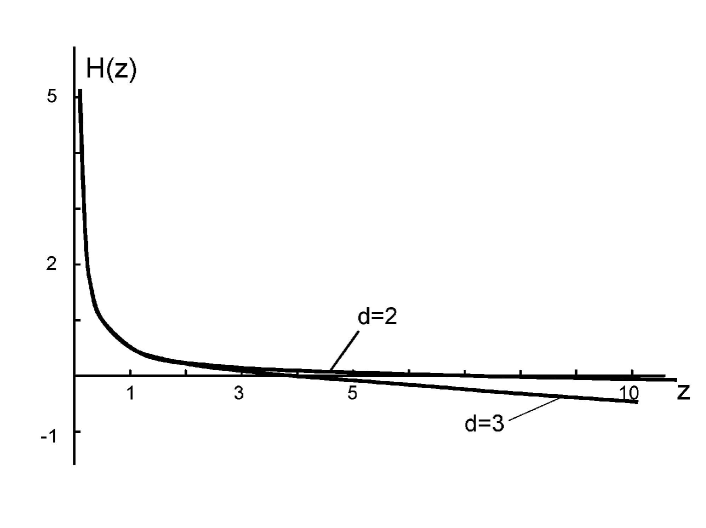
Figure 2: Function $H(z)$ for $b_{1}=0$ in two and three dimensions.

For $d=2$, the constant $b_{1}$ can be eliminated by the change of the scale for $\xi$ (see below) and we can accept $b_{1}=0$. The asymptotics of $H(z)$ for $z\ll 1$ is determined by the last term in Eq. 26, while for $z\gg 1$ the sum in Eq. 26 can be replaced by the integral

$$H(z)=\left\{\begin{array}[]{cc}\displaystyle{\frac{1}{2z}}\,,&\qquad z\ll 1\\ -\displaystyle{\frac{1}{2\pi}}\ln z+const\,,&\qquad z\gg 1\end{array}\right.\,,$$

so we have in variables $y=\xi_{1D}/L$ and $x=\xi/L$

$$y=\left\{\begin{array}[]{cc}(1/\pi)\ln x\,,&\qquad x\gg 1\\ const\cdot x\,,&\qquad x\ll 1\end{array}\right.\,.$$

The relation between $x$ and $y$ for their arbitrary values can be found by the numerical calculation of the sum in (26).

The definition of $\xi_{1D}$ and $\xi$ in the Vollhardt and W${\rm{\ddot{o}}}$lfle theory does not coincide with one used in numerical experiments. In the former case, $\xi^{2}$ (and analogously $\xi^{2}_{1D}$) is defined as an average $\langle r^{2}\rangle$ for the localized eigenfunction $\psi(r)$ [16]. In the latter case, one has in mind the definition through the asymptotic behavior $\exp\{-r/\xi\}$ of the correlation functions, since $\xi_{1D}$ is calculated as inverse to the minimal Lyapunov exponent ; the scale of $\xi$ in numerical experiments is arbitrary from the very beginning. Therefore, in comparison of theory with numerical results the scales of $\xi_{1D}$ and $\xi$ should be chosen from the best agreement; in the log-log coordinates, such fitting reduces to parallel shifts along two axes. The general form of the scaling curve is determined without adjustable parameters.

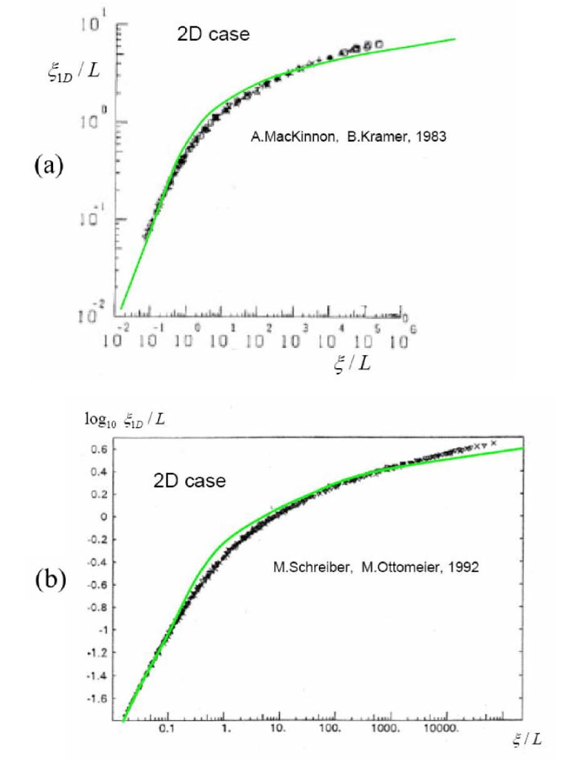
Figure 3: Comparison of the theoretical scaling curve for $d=2$ with numerical results by MacKinnon – Kramer [18, Fig. 2,a] (a) and Schreiber – Ottomeier [19, Fig. 4] (b).

In Fig. 3, the calculated dependence of $\xi_{1D}/L$ on $\xi/L$ is compared with the pioneer results by MacKinnon and Kramer [18] and the subsequent paper by Schreiber and Ottomeier [19], which is cited as the most detailed investigation of the 2D systems in the framework of the given algorithm.

3.3. Three-dimensional case

The given definition of the sum $I_{3}(0)$ implies the choice of cut-off in the form of the cilindrical domain ($|q_{\bot}|<\Lambda$, $|q_{||}|<\Lambda$). It can be also defined for the spherical ($|q|<\Lambda$) and cubical ($|q_{i}|<\Lambda$) regions:

$$I_{3}^{(cub)}(0)=\,\frac{1}{2\pi^{2}L^{d-2}}\sum\limits_{\begin{array}[]{c}{\scriptstyle\vec{s}\neq 0}\\ {\scriptstyle|s_{i}|<\Lambda L/2\pi}\end{array}}\frac{1}{|\vec{s}|}\,{\rm arctg}\left(\frac{\Lambda L}{2\pi|\vec{s}|}\right)$$

$$I_{3}^{(cil)}(0)=\,\frac{1}{2\pi^{2}L^{d-2}}\sum\limits_{\begin{array}[]{c}{\scriptstyle\vec{s}\neq 0}\\ {\scriptstyle|\vec{s}|<\Lambda L/2\pi}\end{array}}\frac{1}{|\vec{s}|}\,{\rm arctg}\left(\frac{\Lambda L}{2\pi|\vec{s}|}\right)$$

$$I_{3}^{(sph)}(0)=\,\frac{1}{2\pi^{2}L^{d-2}}\sum\limits_{\begin{array}[]{c}{\scriptstyle\vec{s}\neq 0}\\ {\scriptstyle|\vec{s}|<\Lambda L/2\pi}\end{array}}\frac{1}{|\vec{s}|}\,{\rm arctg}\left(\frac{\sqrt{(\Lambda L/2\pi)^{2}-|\vec{s}|^{2}}}{|\vec{s}|}\right)$$

Numerically we have for these three cases

$$I_{3}(0)=\left\{\begin{array}[]{cc}\displaystyle{0.0618\Lambda-0.180L^{-1}}&\quad(cube)\\ \displaystyle{0.0573\Lambda-0.314L^{-1}}&\quad(cilinder)\\ \displaystyle{0.0507\Lambda-0.310L^{-1}}&\quad(sphere)\end{array}\right.\,,$$

i. e. value of $b_{1}$ is not universal but depends on the way of cut-off. The change of this constant allows to make the scaling curve more symmetric, or less symmetric; it was chosen from the best agreement , though its variation in the interval $(-0.3,\,0)$ does not affect the results significantly. As in the $2D$ case, the absolute scales for $\xi$ and $\xi_{1D}$ are not fixed by the theory.

Using the asymptotic behavior of $H(z)$

$$H(z)=\left\{\begin{array}[]{cc}\displaystyle{1/2z}\,,&\qquad z\ll 1\\ -A(z-z^{*})\,,&\qquad z\to z^{*}\\ -c_{d}z^{d-2}\,,&\qquad z\gg 1\end{array}\right.\,,$$

one has in variables $y=\xi_{1D}/L$ and $x=\xi/L$

$$y=\left\{\begin{array}[]{cc}2c_{d}/x^{d-2}\,,&\qquad y\gg 1\\ y^{*}\pm B/x^{d-2}\,,&\qquad y\to y^{*}\\ x\,,&\qquad y\ll 1\\ \end{array}\right.\,,$$

where $z^{*}$ and $y^{*}=1/z^{*}$ are values of $z$ and $y$ in the critical point. The same relation, considered in variables $y$ and $1/x$, determines the $L$-dependence of the scaling parameter (Fig. 1) giving two universal curves for $\tau>0$ and $\tau<0$ to which all other curves are reduced by the the scale transformation:

$$y=\frac{\xi_{1D}}{L}=\left\{\begin{array}[]{cc}\sim\tau L^{d-2}\,,&\qquad y\gg 1\\ y^{*}+const\cdot\tau L^{d-2}\,,&\qquad y\to y^{*}\\ \xi/L\,,&\qquad y\ll 1\end{array}\right.\,.$$

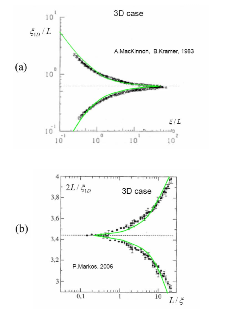
Figure 4: Comparison of the theoretical scaling curves for $d=3$ with numerical results by MacKinnon – Kramer [18, Fig. 2,b] (a) and Markos [1, Fig. 53, right] (b). The values $b_{1}=-0.240$ and $b_{1}=-0.0718$ were used in the former and the latter case correspondingly.

In Fig. 4, the obtained scaling curves are compared with the early results by MacKinnon – Kramer [18] and the more precise results by Markos [1]. In the former case the agreement is satisfactory, in the latter case there is discrepancy on the level of 2 – 3 standard deviations. However, one should have in mind how scaling curves are constructed: the $L$-dependences for different $\tau$ are ”measured” in the interval $(L_{min},L_{max})$, and then they are fitted to each other by a change of the scale (Fig. 5).

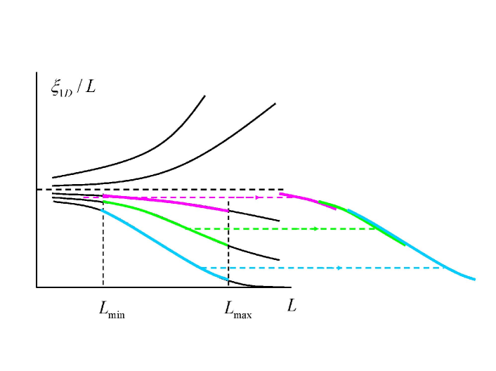
Figure 5: Construction of scaling curves.

The full scaling curve is never present in one experiment, and only separate fragments of it are measured. It is clear from Fig. 4,b that the change of the scale along the horizontal axis (reducing to a parallel shift in the logarithmic coordinates) allows to obtain satisfactory fits for the left, right or middle portion of the curve. It looks, there are no serious contradictions with the Vollhardt and W${\rm{\ddot{o}}}$lfle theory on the level of raw data.

4. DISCUSSION OF THE SITUATION AT $D=3$

The interesting question arises: if the Vollhardt and W${\rm{\ddot{o}}}$lfle theory describes the raw data successfully, then why all numerical experiments give $\nu>1$ for $d=3$ ?

The history of this question goes back to two papers [17] and [18] by MacKinnon and Kramer, based on the same array of the data. The first of them gives the result

$$\nu=1.2\pm 0.3\,,$$

compatible with the value $\nu=1$; the second paper confirms this result for a certain fitting procedure, but reports the ”more precise” result

$$\nu=1.50\pm 0.05\,,$$

corresponding to the most extremal of present-day values. The first result is based on the analysis of the scaling curve, whose compatibility with the Vollhardt and W${\rm{\ddot{o}}}$lfle theory is clear from Fig. 4,a and is confirmed by the authors themselves. Further, they indicate that scaling is not satisfactory in the small vicinity of the critical point, and this vicinity was discarded in their treatment. In fact, such situation is natural, because the small vicinity of the transition is strongly affected by scaling corrections (see Eq. 23); the latter are small in magnitude but should be compared with the small value of $\tau$. However, the authors of [17, 18] estimated this situation as internally inconsistent and suggested another treatment procedure, which is specially based on the analysis of that small region where scaling is absent. Already at this stage it is possible to understand that the latter procedure is not satisfactory.

Indeed, using the systems of the restricted size $L$, one can work straightforwardly only in the regime $\xi\mathbin{\lower 3.0pt\hbox{$\hbox to0.0pt{\raise 5.0pt\hbox{$\char 60\relax$}\hss}\mathchar 29208\relax$}}L$, since in another case the correlation functions are strongly affected by finiteness of the system. The use of finite-size scaling allows ”to jump above the head” and to advance in the region $\xi\mathbin{\lower 3.0pt\hbox{$\hbox to0.0pt{\raise 5.0pt\hbox{$\char 62\relax$}\hss}\mathchar 29208\relax$}}L$; however, it is possible only if (a) scaling exists theoretically, and (b) it is observed empirically. If any of two conditions is violated, no such advancement is possible, and one is unable to obtain any experimental information on the large $\xi$ region; any manipulations in this region become irrelevant. This conclusion is valid in respect of the result (36), since absence of scaling is admitted by the authors. The same conclusion follows from the common sense: if value $\nu=1$ is compatible with the scaling curve, then all the more it is compatible with the raw data (see the end of Sec. 3). However, this value is rejected by the result (36), and hence the latter should be qualified as essentially incorrect.

The indicated tendencies was continued in other papers. The treatment based on the scaling curves gave rather conservative estimates , not very different from (35). The results close to (36) were stabilized only when the control of scaling ceased to be imperative and the analysis of small vicinity of the critical point was generally accepted.

The latter procedure is based on representation of (4) in the form

$$\frac{\xi_{1D}}{L}=F\left(\frac{L^{1/\nu}}{\xi^{1/\nu}}\right)=F\left(\tau L^{1/\nu}\right)\approx y^{*}+A\tau L^{1/\nu}+\ldots\,$$

i. e. the regular expansion in $\tau$ is used, motivated by the absence of phase transitions in quasi-1D systems; then the derivative over $\tau$ behaves as $L^{1/\nu}$ and gives the exponent $\nu$ straightforwardly. Such treatment is correct if the scaling relation (4) is exact. However, it is not exact: linearization of (23) gives

$$\frac{\xi_{1D}}{L}=y^{*}+A\left(\frac{L}{a}\right)^{d-2}\left[\tau-c\frac{a^{2}}{\xi_{1D}^{2}}\right]+O\left(\frac{a}{L}\right)\,.$$

Differentating over $\tau$ and excluding $(\xi_{1D})^{\prime}_{\tau}$ from the right-hand side in the iterative manner, one has

$$\left(\frac{\xi_{1D}}{L}\right)^{\prime}_{\tau}=A_{0}L^{d-2}+A_{1}L^{d-6}\,.$$

Producing subsequent iterations and taking into account further corrections to scaling, one have the following structure of the result

$$\frac{\xi_{1D}}{L}-y^{*}=\tau\left\{A_{0}L^{1/\nu}+A_{1}L^{\omega_{1}}+A_{2}L^{\omega_{2}}+\ldots\right\}+B_{1}L^{-y_{1}}+B_{2}L^{-y_{2}}+\ldots\,,$$

which can be obtained from the general considerations based on the Wilson renormalization group [2].

In three dimensions, the main scaling correction in (39) reduces to constant, and hence

$$\frac{\xi_{1D}}{L}-y^{*}=A\tau\left(L+L_{0}\right)\,,$$

where the terms dissapearing at $L\to\infty$ are neglected. It is clear from Fig. 6,a, that numerical data by Markos [1] are excellently fitted by (41). The author himself interpreted them in accordance with (37) and also had the good fitting (Fig. 6,b).

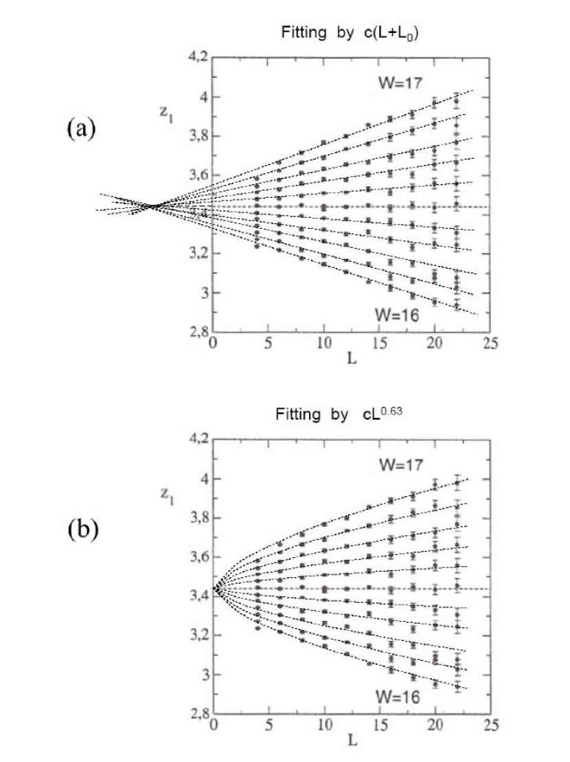
Figure 6: Numerical data by Markos for $z_{1}=2L/\xi_{1D}$ in the small vicinity of the critical point [1, Fig. 53, left] and their fitting by dependences $(L+L_{0})$ (a) and $L^{0.63}$ (b).

Such ambiguity of interpretation has a general character. If the combination $A_{1}L^{\beta_{1}}+A_{2}L^{\beta_{2}}$ can be linearized in the log-log coordinates with the average slope $(\beta_{1}+\beta_{2})/2$ and the accuracy $\epsilon$, then variation $\beta_{1}\to\beta_{1}+\delta$, $\beta_{2}\to\beta_{2}-\delta$ preserves linearity on the same level of accuracy, till $|\delta|\mathbin{\lower 3.0pt\hbox{$\hbox to0.0pt{\raise 5.0pt\hbox{$\char 60\relax$}\hss}\mathchar 29208\relax$}}|\beta_{1}-\beta_{2}|/2$. If several terms are retained in (40), the situation becomes not controllable at all: non-linear fitting with minimization of $\chi^{2}$ reveals the huge number of minima, and the deepest of them is not necessary correct; a vicinity of any minimum is acceptable if it is satisfied to the $\chi^{2}$ criterion. Analysis of all such minima is impossible, and there is no honest procedure to deal with such situation . In conclusion, the conventional treatment is heavily based on the assumption, that only the main term in (40) is essential; the problem of fitting becomes hopeless, if additional terms are not negligible.

In the framework of the Vollhardt and W${\rm{\ddot{o}}}$lfle theory, we have a completely consistent picture. The quantity $L_{0}$ violates scaling and empirically has rather large value, $L_{0}\approx 5$ (in lattice units). The good scaling is possible only for $L\gg 5$, and even for the largest systems ($L=20\div 30$) deviations of scaling are described by the parameter $L_{0}/L\sim 0.2$; so discrepancies in Fig. 4,b should not be of any surprise. The theoretical value of $L_{0}$ is of the order $\Lambda^{-1}$ with the coefficient depending on the way of cut-off; it is essential that $L_{0}$ is positive and limited from below by the atomic scale.

5. SCALING FOR HIGHER DIMENSIONS

5.1. Dimensions $d>4$

For $d\geq 4$, the sum $I_{2}(m)$ is divergent at the upper limit and the cut-off parameter $\Lambda$ cannot be considered as infinite. For the accurate trasformation, we introduce the scale $\Lambda_{1}$ such as

$$m\ll\Lambda_{1}\ll\Lambda$$

and divide summation in $I_{2}(m)$ into two regions $|q_{\bot}|<\Lambda_{1}$ and $|q_{\bot}|>\Lambda_{1}$. In the first region we use that $|q_{\bot}|\ll\Lambda$, so as

$$I_{2}^{(1)}(m)=-m^{2}\frac{1}{2L^{d-1}}\,\sum\limits_{\begin{array}[]{c}{\scriptstyle q_{\bot}\neq 0}\\ {\scriptstyle|q_{\bot}|<\Lambda_{1}}\end{array}}\,\frac{1}{|q_{\bot}|\,\sqrt{m^{2}+q_{\bot}^{2}}\,\left(|q_{\bot}|+\sqrt{m^{2}+q_{\bot}^{2}}\right)}$$

and

$$I_{2}^{(1)}(m)=\left\{\begin{array}[]{cc}{\displaystyle-m^{2}\left\{\frac{K_{d-1}\Lambda_{1}^{d-4}}{4(d-4)}+O\left(m^{d-4}\right)\right\}}\,,&m\mathbin{\lower 3.0pt\hbox{$\hbox to0.0pt{\raise 5.0pt\hbox{$\char 62\relax$}\hss}\mathchar 29208\relax$}}L^{-1}\\ {\displaystyle-m^{2}\left\{\frac{K_{d-1}\Lambda_{1}^{d-4}}{4(d-4)}+O\left(L^{4-d}\right)\right\}}\,,&m\mathbin{\lower 3.0pt\hbox{$\hbox to0.0pt{\raise 5.0pt\hbox{$\char 60\relax$}\hss}\mathchar 29208\relax$}}L^{-1}\end{array}\right.\,,$$

i. e. the result is obtained analytically (in the main approximation) for the arbitrary relation between $m$ and $L^{-1}$. Indeed, for $m\gg L^{-1}$ the sum is estimated by the integral, which is converging at the lower limit already for $m=0$; so a finiteness of $m$ gives only small corrections. In the case $m\mathbin{\lower 3.0pt\hbox{$\hbox to0.0pt{\raise 5.0pt\hbox{$\char 60\relax$}\hss}\mathchar 29208\relax$}}L^{-1}$, the main effect from a finiteness of $L$ is related with the absence of the term $q_{\bot}=0$, which can be estimated as restriction $|q_{\bot}|\mathbin{\lower 3.0pt\hbox{$\hbox to0.0pt{\raise 5.0pt\hbox{$\char 62\relax$}\hss}\mathchar 29208\relax$}}L^{-1}$ in the integral approximation.

In the region $|q_{\bot}|>\Lambda_{1}$ we make use of condition $|q_{\bot}|\gg m$ and produce expansions in $m/|q_{\bot}|$; after separation the factor $m^{2}$ we can set $m=0$ in the sum and estimate it by transformation to the integral

$$I_{2}^{(2)}(m)=m^{2}\frac{K_{d-1}\Lambda_{1}^{d-4}}{4(d-4)}-cm^{2}\Lambda^{d-4}$$

where $c$ depends on the way of cut-off; dependence on $\Lambda_{1}$ dissapears in the sum $I_{2}^{(1)}+I_{2}^{(2)}$.

The results for $I_{1}(m)$ and $I_{3}(0)$ are the same as in Sec. 3. The self-consistency equation takes the form

$$\tau\Lambda^{d-2}=\frac{1}{L^{d-2}}\,\frac{1}{2mL}-cm^{2}\Lambda^{d-4}$$

Substituting $\tau\sim\xi^{-2}$ and introducing variables

$$y=\frac{\xi_{1D}}{L}\left(\frac{a}{L}\right)^{(d-4)/3}\,,\qquad x=\frac{\xi}{L}\left(\frac{a}{L}\right)^{(d-4)/3}\,,$$

we obtain the scaling relation in the analytical form

$$\pm\frac{1}{x^{2}}=y-\frac{1}{y^{2}}$$

where all coefficients are made equil to unity by redefinition of the scales for $\xi_{1D}$ and $\xi$. Relations (46 ,47) contain the atomic scale $a$, as was expected from non-renormalizability of theory (Sec. 1).

According to (46 ,47), the role of the scaling parameter is played by the quantity $y$ instead of $\xi_{1D}/L$; the $L$-dependence of $y$ is analogous to Fig. 1, i. e. all curves corresponding to $\tau>0$ and $\tau<0$ can be reduced to two universal ones by the scale transformation. The transition point corresponds to $y=1$, so as

$$\frac{\xi_{1D}}{L}\sim\left(\frac{L}{a}\right)^{(d-4)/3}\,,\qquad\tau=0$$

and the critical point cannot be fixed by the condition $\xi_{1D}/L=const$.

5.2. Four-dimensional case

In the case $d=4$ we have analogously

$$I_{2}(m)=\left\{\begin{array}[]{cc}{\displaystyle-c_{4}\,m^{2}\ln\frac{\Lambda}{m}+O\left(1\right)\,,}&m\mathbin{\lower 3.0pt\hbox{$\hbox to0.0pt{\raise 5.0pt\hbox{$\char 62\relax$}\hss}\mathchar 29208\relax$}}L^{-1}\\ {}\hfil\\ {\displaystyle-c_{4}\,m^{2}\ln(\Lambda L)+O\left(1\right)}\,,&m\mathbin{\lower 3.0pt\hbox{$\hbox to0.0pt{\raise 5.0pt\hbox{$\char 60\relax$}\hss}\mathchar 29208\relax$}}L^{-1}\end{array}\right.\,,$$

i. e. two results differ by $\ln(mL)$, which reduces to the double-logarithmic quantity in the actual region (see below). Neglecting such quantities, we can obtain scaling also for $d=4$. The self-consistency equation has a form

$$\tau\Lambda^{2}=\frac{1}{2mL^{3}}-c_{4}\,m^{2}\ln\frac{\Lambda}{m}$$

and after changing to $\xi$ and $\xi_{1D}$

$$\pm\frac{c_{4}}{\xi^{2}}\ln(\xi/a)=\frac{\xi_{1D}}{2L^{3}}-\frac{c_{4}}{\xi_{1D}^{2}}\ln(\xi_{1D}/a)$$

The scaling relation (47) is obtained in variables

$$y=\frac{\xi_{1D}}{L}\left[\ln(L/a)\right]^{-1/3}\,,\qquad x=\frac{\xi}{\left[\ln(\xi/a)\right]^{1/2}}\frac{\left[\ln(L/a)\right]^{1/6}}{L}\,,$$

i. e. the scaling parameter $y$ is logarithmically modified in comparison with $\xi_{1D}/L$ and should be considered as a function of ”the modified length” $\mu(L)=L\left[\ln(L/a)\right]^{-1/6}$; then all dependences become analogous to Fig. 1 and a change of the scale for $\mu(L)$ allows to reduce them to two universal curves for $\tau>0$ and $\tau<0$. The critical point corresponds to $y=const$, so as

$$\frac{\xi_{1D}}{L}\sim\left(\ln\frac{L}{a}\right)^{1/3}\,,\qquad\tau=0$$

i. e. parameter $\xi_{1D}/L$ grows logarithmically in the transition point.

5.3. Modified scaling for $d=4-\epsilon$

From the methodical point of view, it is interesting to derive the modified scaling for $d=4-\epsilon$; in this case, the sum $I_{2}(m)$ converges formally at the upper limit, but this convergence is slow and a finiteness of $\Lambda$ gives the essential effect. Analogously to (49) we have

$$I_{2}(m)=\left\{\begin{array}[]{cc}{\displaystyle-c_{4}\,m^{2}\frac{m^{-\epsilon}-\Lambda^{-\epsilon}}{\epsilon}\,,}&m\mathbin{\lower 3.0pt\hbox{$\hbox to0.0pt{\raise 5.0pt\hbox{$\char 62\relax$}\hss}\mathchar 29208\relax$}}L^{-1}\\ {\displaystyle-c_{4}\,m^{2}\frac{L^{\epsilon}-\Lambda^{-\epsilon}}{\epsilon}}\,,&m\mathbin{\lower 3.0pt\hbox{$\hbox to0.0pt{\raise 5.0pt\hbox{$\char 60\relax$}\hss}\mathchar 29208\relax$}}L^{-1}\end{array}\right.\,,$$

and the scaling relation (47) is obtained in variables

$$y=\frac{\xi_{1D}}{L}\left[\frac{\epsilon}{1-(L/a)^{-\epsilon}}\right]^{1/3}\,,\qquad x=\frac{\epsilon^{1/3}(\xi/a)}{\left[(\xi/a)^{\epsilon}-1\right]^{1/2}}\,\frac{\left[1-(L/a)^{-\epsilon}\right]^{1/6}}{(L/a)^{1-\epsilon/2}}\,.$$

Once again we have the modified scaling parameter $y$ and ”the modified length” $\mu(L)=L^{1-\epsilon/2}\left[1-(L/a)^{-\epsilon}\right]^{-1/6}$, in terms of which the dependences of Fig. 1 are recovered. In the critical point we have $y=1$ and

$$\frac{\xi_{1D}}{L}=\left[\frac{1-(L/a)^{-\epsilon}}{\epsilon}\right]^{1/3}\,=\left\{\begin{array}[]{cc}{\displaystyle\left[\ln(L/a)\right]^{1/3}\,,}&\ln(L/a)\mathbin{\lower 3.0pt\hbox{$\hbox to0.0pt{\raise 5.0pt\hbox{$\char 60\relax$}\hss}\mathchar 29208\relax$}}1/\epsilon\\ {}\hfil\\ {\displaystyle\left(1/\epsilon\right)^{1/3}}\,,&\ln(L/a)\mathbin{\lower 3.0pt\hbox{$\hbox to0.0pt{\raise 5.0pt\hbox{$\char 62\relax$}\hss}\mathchar 29208\relax$}}1/\epsilon\end{array}\right.\,,$$

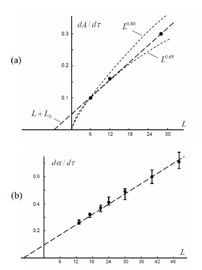
Figure 7: Fitting by dependence $(L+L_{0})$ (dashed line) for numerical data, based on the level statistics: (a) Data by Zharekeshev and Kramer [27]. The points correspond to the average derivatives of the scaling parameter $A$ (arbitrary units), determined from Fig. 4 of [27] in the interval $16<W<17$. A statistical error related with each point can be estimated very conservatively (see Table in [2]) due to the irregular character of curves given in the indicated figure; uncertainty allowed by the authors themselves corresponds to the gap between dependences $L^{0.80}$ and $L^{0.65}$, determining the upper and lower bound of the result for the critical exponent, $\nu=1.40\pm 0.15$. (b) Data obtained by Schreiber’ group [43]; the points correspond to the derivative of the scaling parameter $\alpha$ (arbitrary units) determined by the slope of solid lines in the inset of Fig. 3 in [43]; their uncertainty is obtained by variation of the slope allowed by the size of experimental points.

i. e. parameter $\xi_{1D}/L$ grows logarithmically till the large length scale $L_{0}\sim a\exp\{const/\epsilon\}$, and then saturates at the constant value. Such kind of scaling is useful as an alternative treatment for $d=3$, in order to investigate the systematic errors related with the possible existence of the large length scale. In this case the parameter $a$ in fact corresponds to $L_{0}$ and can be essentially different from the lattice constant; it should be adjusted from the condition of the best quality of scaling. There is no need to be bound by Eq. 47, which is valid for small $\epsilon$; it is more reasonable to determine the relation $y=F(x)$ empirically. As for expressions (55), their extrapolation to $\epsilon=1$ does not present any problem, since for $L,\,\,\xi\gg a$ the modified scaling safely reduces to the usual one (see Eq. 4). In fact, it is identical to (4) if no large scale $L_{0}$ is present. However, in the presence of the large length $L_{0}$ such scaling is more adequate than (4).

6. CONCLUSION

The above analysis allows to conclude that the Vollhardt–W${\rm{\ddot{o}}}$lfle theory does not have essential contradictions with numerical results on the level of raw data. The different critical behavior reported usually in numerical papers originates from the fact, that some time ago the pure ”experimental” approach to the problem was rejected and replaced by phenomenological analysis, which is practically hopeless in the corresponding region. In particular, dependence $L+L_{0}$ with $L_{0}>0$ is interpreted as $L^{1/\nu}$ with $\nu>1$.

We have restricted our discussion by the widespread variant of finite-size scaling, based on application of auxiliary quasi-1D systems. Apart it, another algorithms are used, based on the level statistics [20], the conductance distribution, the mean conductance, etc. [1]. The scaling curves calculated above are not universal and cannot be used for comparison with such results. The scaling for higher dimensions is also not universal: for example, another behavior in the critical point is expected for the Thouless parameter [40]. The only exclusion is the result (40), which remains unchanged in all cases. Indeed, this result can be obtained from the general arguments based on the Wilson renormalization group [2]; the exponents $\omega_{1}$, $\omega_{2}$, $y_{1}$, $y_{2},\,\ldots$ are determined by scaling dimensions of irrelevant parameters and hence are universal. Correspondingly, the result (41) is unchanged, which explain the origin of the effective values $\nu>1$ (Fig. 7).

Fig.7,a can be considered as an etalon illustration, corresponding to most of numerical papers. Indeed, there is an overall consensus that data for $L\mathbin{\lower 3.0pt\hbox{$\hbox to0.0pt{\raise 5.0pt\hbox{$\char 60\relax$}\hss}\mathchar 29208\relax$}}5$ fall out of the scaling picture and should be discarded; large systems with $L\mathbin{\lower 3.0pt\hbox{$\hbox to0.0pt{\raise 5.0pt\hbox{$\char 62\relax$}\hss}\mathchar 29208\relax$}}30$ are practically never used; the error corridor between dependences $L^{0.80}$ and $L^{0.65}$ corresponds to the typical accuracy of numerical papers. Fig.7,b illustrates one of the rare papers treating the systems of the record size [43]. Finally, Fig.8 shows the rare example of high-precision data [44].

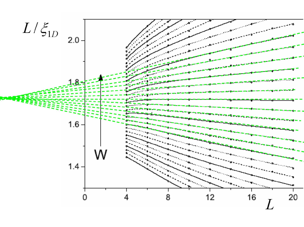
Figure 8: High-precision data by Kramer et al [44] and their fitting by dependence $C(L+L_{0})$ (green lines). Black solid and dashed lines correspond to the ambiguous many-parameter treatment with $\nu=1.57$. Corrections $O(a/L)$ are visible for small $L$.

Our final remark is as follows. Even if subsequent investigations reveal that the Vollhardt and W${\rm{\ddot{o}}}$lfle theory is not exact, nevertheless no confidence can be given to the present-day estimates of the exponent $\nu$ [17]–[31]. Fig. 6 clearly demonstrates that values $\nu\approx 1.6$ and $\nu=1$ are equally compatible with the raw data, and hence the treatment procedure is extremely ambiguous.

References

• [1] P. Markos, acta physica slovaca 56, 561 (2006); cond-mat/0609580.
• [2] I.Β M.Β Suslov, cond-mat/0105325, cond-mat/0106357
• [3] I.Β M.Β Suslov, cond-mat/0610744.
• [4] D. Vollhardt, P. W$\ddot{o}$lfle, Phys. Rev. B 22, 4666 (1980); Phys. Rev. Lett. 48, 699 (1982). D. Vollhardt, P. W$\ddot{o}$lfle, in Modern Problems in Condensed Matter Sciences, ed. by V. M. Agranovich and A. A. Maradudin, v. 32, North-Holland, Amsterdam (1992).
• [5] A. Kawabata, Solid State Commun. 38, 823 (1981). B. Shapiro, Phys. Rev. B 25, 4266 (1982). A. V. Myasnikov, M. V. Sadovskii, Fiz. Tverd. Tela (Leningrad) 34, 3569 (1982).
• [6] I. M. Suslov, Usp. Fiz. Nauk 168, 503 (1998) [Physics-Uspekhi 41, 441 (1998)]; cond-mat/9912307.
• [7] F. Wegner, Z. Phys. B 35, 207 (1979); L. Sch$\ddot{a}$fer, F. Wegner, Z. Phys. B 38, 113 (1980). S. Hikami, Phys. Rev. B 24, 2671 (1981). K. B. Efetov, A. I. Larkin, D. E. Khmelnitskii, Zh. Eksp. Teor. Fiz. 79, 1120 (1980) [Sov. Phys. JETP 52, 568 (1980)]. K. B. Efetov, Adv. Phys. 32, 53 (1983).
• [8] E. Abrahams, P. W. Anderson, D. C. Licciardello, and T. V. Ramakrishman, Phys. Rev. Lett. 42, 673 (1979).
• [9] H. Kunz, R. Souillard, J. de Phys. Lett. 44, L411 (1983).
• [10] K. B. Efetov, Zh. Eksp. Teor. Fiz. 93, 1125 (1987); 94, 357 (1988) [Sov. Phys. JETP 66, 634 (1987); 67, 199 (1988)].
• [11] B. Shapiro, Phys. Rev. Lett. 50, 747 (1983).
• [12] D. Belitz, T. R. Kirkpatrick, Rev. Mod. Phys., 66, 261 (1994).
• [13] N. G. Zhdanova, M. S. Kagan, E. G. Landsberg, JETP 90, 662 (2000).
• [14] H. Kunz, R. Souillard, J. de Phys. Lett. 44, L506 (1983).
• [15] F. Wegner, Nucl. Phys. B 316, 663 (1989).
• [16] I. M. Suslov, Zh. Eksp. Teor. Fiz. 108, 1686 (1995) [JETP 81, 925 (1995)]; cond-mat/0111407.
• [17] A. MacKinnon, B. Kramer, Phys. Rev. Lett. 47, 1546 (1981).
• [18] A. MacKinnon, B. Kramer, Z. Phys. 53, 1 (1983).
• [19] M. Schreiber, M. Ottomeier, J.Phys.: Condens. Matter 4, 1959 (1992).
• [20] B. I. Shklovskii, B. Shapiro, B. R. Sears et al, Phys. Rev. B 47, 11487 (1993).
• [21] I. Kh. Zharekeshev, B. Kramer, Phys. Rev. B 51, 17 239 (1995).
• [22] B. Kramer, K. Broderix, A. MacKinnon, M. Schreiber, Physica A 167, 163 (1990).
• [23] E. Hofstetter, M. Schreiber, Europhys. Lett. 21, 933 (1993).
• [24] A. MacKinnon, J.Β Phys.: Condens. Matter 6, 2511 (1994).
• [25] M. Schreiber, H. Grussbach, Phys. Rev. Lett. 76, 1687 (1996).
• [26] I. Kh. Zharekeshev, B. Kramer, Phys. Rev. B 51, 17239 (1995).
• [27] I. Kh. Zharekeshev, B. Kramer, Phys. Rev. Lett. 79, 717 (1997).
• [28] I. Kh. Zharekeshev, B. Kramer, Ann. Phys. (Leipzig) 7, 442 (1998).
• [29] K. Slevin, T. Ohtsuki, Phys. Rev. Lett. 82, 382 (1999).
• [30] P. Markos, J. Phys. A: Math&Gen 33, L393 (2000).
• [31] P. Markos, M. Heneke, J. Phys.: Condens. Matter 6, L765 (1994).
• [32] I. M. Suslov, Zh. Eksp. Teor. Fiz. 128, 768 (2005) [JETP 101, 661 (2005)]; cond-mat/0504557.
• [33] I. M. Suslov, Zh. Eksp. Teor. Fiz. 129, 1064 (2006) [JETP 102, 938 (2006)]; cond-mat/0512708.
• [34] J. L. Pichard, G. Sarma, J. Phys. C: Solid State Phys. 14, L127 (1981); 14, L617 (1981).
• [35] Ma S., Modern Theory of Critical Phenomena, Reading, Mass.: W.A.Benjamin, Advanced Book Program, 1976.
• [36] A. Nitzan, K. F. Freed, M. N. Cohen, Phys. Rev. B 15, 4476 (1977).
• [37] M. V. Sadovskii, Usp. Fiz. Nauk 133, 223 (1981) [Sov. Phys. Usp. 24, 96 (1981)];
• [38] N. N. Bogolyubov, D. V. Shirkov, Introduction to the Theory of Quantized Fields, New York: John Wiley, 1980.
• [39] E. Brezin, J. C. Le Guillou, J. Zinn-Justin, in Phase Transitions and Critical Phenomena, ed. by C. Domb and M. S. Green, Academic, New York (1976), Vol. VI.
• [40] I. M. Suslov, Zh. Eksp. Teor. Fiz. 113, 1460 (1998) [JETP 86, 798 (1998)]; cond-mat/0007027.
• [41] T. Brandes, B. Huckestein, L. Schweitzer, Ann. Phys. 5, 633 (1996).
• [42] I. M. Suslov, cond-mat/0612654.
• [43] F. Milde, R. A. Romer, M. Schreiber, Phys. Rev. B 61, 6028 (2000).
• [44] B. Kramer, A. MacKinnon, K. Slevin, T. Ohtsuki, arXiv: 1004.0285