Abstract

The hydrostatic primitive equations (HPE) form the basis of most numerical weather, climate and global ocean circulation models. Analytical (not statistical) methods are used to find a scaling proportional to $\left(Nu\,Ra\,Re\right)^{1/4}$ for the range of horizontal spatial sizes in HPE solutions, which is much broader than currently achievable computationally. The range of scales for the HPE is determined from an analytical bound on the time-averaged enstrophy of the horizontal circulation. This bound allows the formation of very small spatial scales, whose existence would excite unphysically large linear oscillation frequencies and gravity wave speeds.

The hydrostatic primitive equations (HPE) have been the foundation of most numerical weather, climate and global ocean circulation calculations for many decades [1, 2, 3, 4, 5]. In practice, modern computational power can handle integrations of these on global horizontal grids ranging in size between 15km and 60km, which correspond respectively to one-eighth degree and one-half degree in latitude and longitude at the equator. This limitation raises the long-standing question, “Can numerical simulations at these grid sizes adequately predict climate and other natural phenomena that occur on the much wider range of scales observed in Nature?” See Figure 1.

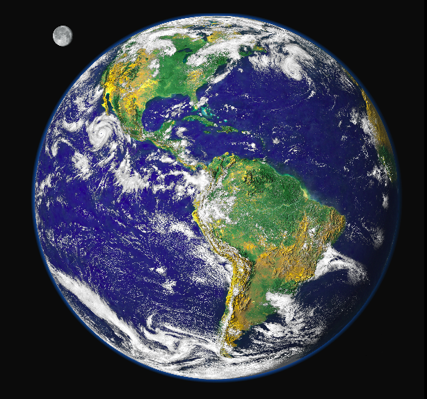
Figure 1: A NASA image [6] illustrates the large range of fluid scales that exist in atmospheric circulation. The oceanic range of scales is similar, but is not so easily observed.

Important as it may be, this long-standing question is not addressed here. Rather, two questions are addressed associated with the HPE model itself. Namely, “What range of scales is available for solutions of the HPE?” and “What scaling law governs the size of horizontal HPE excitations in terms of the system parameters?” These dimensionless parameters are $Nu$, $Ra$ and $Re$, associated with the names of Nusselt, Rayleigh and Reynolds, respectively.

The HPE differ from the three-dimensional Navier-Stokes equations in incorporating rotation, stratification, and imposing vertical hydrostatic balance. The latter is often regarded as the most accurate of the various assumptions used in large-scale computations of the climate, weather and ocean circulation. The hydrostatic assumption determines the pressure from the weight of the water above a given point, independently of its state of motion. This changes the nature of the dynamics, because the vertical velocity is determined from incompressibility, rather than from its own evolution equation.

Unlike the Navier-Stokes equations, solutions of the HPE have been proved to be regular by Cao and Titi [7]. Moreover, the HPE have also been shown to possess a global attractor [8]. Although its solutions are regular, the HPE system may potentially possess a vast range of sizes of excitations [9]. While Kolmogorov introduced the $Re^{3/4}$ scaling law for the range of spatial sizes of excitations in incompressible fluid flows by using statistical methods [10], the present note will use analytical methods to show that a scaling law exists, proportional to $\left(Nu\,Ra\,Re\right)^{1/4}$, for the range of horizontal spatial sizes in solutions of the HPE, with similar boundary conditions to those of Cao and Titi [7]. This result demonstrates that HPE excitations are possible at scales that are many orders of magnitude smaller than are possible in present numerical resolutions.

A dimensionless version of the HPE may be expressed in terms of two sets of velocity vectors involving the horizontal velocities $u,\,v$ and the vertical velocity $w$ [11]

$$\mbox{\boldmath$V$}(x,y,z,t)=(u,\,v,\,\varepsilon w),\qquad\mbox{\boldmath$v$}=(u,\,v,\,0).$$ (1)

Under the constraint of incompressibility, $\mbox{div}\,\mbox{\boldmath$V$}=0$, these satisfy

$$\varepsilon\left(\partial_{t}+\mbox{\boldmath$V$}\cdot\nabla\right)u-v=\varepsilon Re^{-1}\Delta u-\partial_{x}P,$$ (2)

$$\varepsilon\left(\partial_{t}+\mbox{\boldmath$V$}\cdot\nabla\right)v+u=\varepsilon Re^{-1}\Delta v-\partial_{y}P.$$ (3)

Here $\varepsilon$ is the Rossby number, $Re=U_{0}L/\nu$ is the Reynolds number and $P$ the pressure.

As mentioned earlier, HPE has no evolution equation for the vertical velocity component $w$. Instead, this variable is determined (diagnosed) from the incompressibility condition, $\hbox{div}\,\mbox{\boldmath$V$}=0$. The $z$-derivative of the pressure field $P$ and the dimensionless temperature $\Theta$ enter through the equation for hydrostatic balance

$$a_{0}\Theta+\partial_{z}P=0\,.$$ (4)

The coefficient $a_{0}=(\varepsilon\sigma^{-1}\alpha_{a}^{-2})R{a}Re^{-2}$ arises from non-dimensionalization of the equations. Here $\sigma=\nu/\kappa$ is the Prandtl number (the ratio of viscosity $\nu$ and thermal diffusivity $\kappa$), $Ra$ is the Rayleigh number, defined by $R{a}=g\alpha T_{0}H^{3}(\nu\kappa)^{-1}$, $g$ is acceleration of gravity, $\alpha$ is volumetric expansion coefficient, $T_{0}$ is a typical temperature difference and $\alpha_{a}=H/L$ is the aspect ratio of the cylindrical domain. When (2), (3) and (4) are combined, an evolution equation for the hydrostatic velocity field $\mbox{\boldmath$v$}=(u,\,v,\,0)$ results as

$$\varepsilon\left(\partial_{t}+\mbox{\boldmath$V$}\cdot\nabla\right)\mbox{\boldmath$v$}+\mbox{\boldmath$\hat{k}$}\times\mbox{\boldmath$v$}+a_{0}\mbox{\boldmath$\hat{k}$}\Theta=\varepsilon Re^{-1}\Delta\,\mbox{\boldmath$v$}-\nabla P,$$ (5)

which is taken in tandem with the incompressibility condition $\hbox{div}\,\mbox{\boldmath$V$}=0$. The dimensionless temperature $\Theta$ (the source of buoyancy) evolves according to

$$\left(\partial_{t}+\mbox{\boldmath$V$}\cdot\nabla\right)\Theta=(\sigma Re)^{-1}\Delta\Theta+q\,,$$ (6)

in which nondimensional $q$ specifies heat sources, or sinks. The domain $\Omega$ is taken to be a cylinder of radius $L$ and height $H$. The vertical velocity and vertical flux of horizontal momentum both vanish on its flat upper and lower cylinder surfaces ($z=0,\,H$). That is, $w=0$ and $u_{z}=v_{z}=0$ on the boundary. The variables are all taken to be periodic on the sides of the cylinder.

Linearizing the HPE in (5) and (6), and their non-hydrostatic equivalent (which has the dynamics of $w$ restored), leads to well-known dispersion relations [13], which are illustrated in Figure 2. The essence of these dispersion curves is that without the frequency cut-off enforced by the buoyancy terms in the non-hydrostatic equations, the HPE admit unphysically high gravity wave frequencies at small scales. Moreover, these HPE gravity waves propagate at a fixed phase speed in the limit of small scales, while in reality gravity waves at these scales cease to propagate at all.

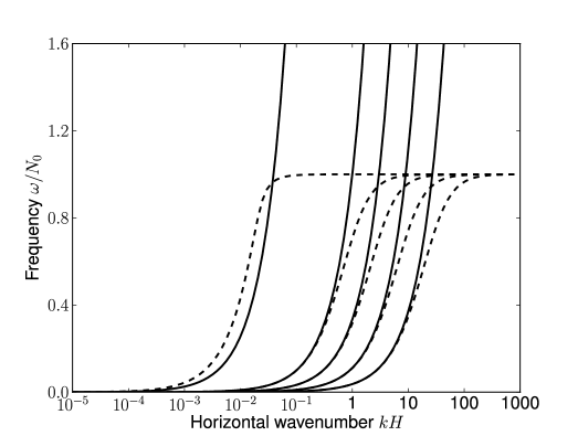
Figure 2: This comparison of linear mode dispersion relations for the hydrostatic primitive equations (solid curves) with those of the exact nonhydrostatic equations (dashed curves) for oceanic conditions shows that the primitive equations admit very high fluctuation frequencies, especially at high horizontal wave numbers. In contrast, the dispersion relation for the nonhydrostatic equations limits properly to the buoyancy frequency, regardless of how high the horizontal wave number becomes. Oceanic parameters are taken as $c_{s}=1500ms^{-1}$, $H=10^{3.5}m$, $N_{0}=0.01s^{-1}$ where the appropriate normalizing length scale $H$ is the mean ocean depth. The multiple curves correspond to different choices of vertical wave number, $mH\in[0,1,3,9,27]$, increasing from the left. The value $m=0$ is the barotropic mode and the others are baroclinic.

1 An estimate for the resolution length

Taking the inner product of the divergence-free velocity $V$ with the motion equation (5) gives an equation for the rate of change of the kinetic energy of horizontal motion

$$\frac{1}{2}\frac{d~{}}{dt}\int_{\Omega}|\mbox{\boldmath$v$}|^{2}\,d\mathcal{V}=\int_{\Omega}\left(Re^{-1}\mbox{\boldmath$V$}\cdot\Delta\mbox{\boldmath$v$}-a_{0}w\Theta\right)d\mathcal{V}$$ (7)

in which $d\mathcal{V}$ is the volume element and surface terms integrate to zero under the present boundary conditions. For the Navier-Stokes equations it is normal practice to use the energy dissipation rate $\nu\left<\int_{\Omega}|\mbox{\boldmath$\omega$}|^{2}\,d\mathcal{V}\right>$ based on the full vorticity $\mbox{\boldmath$\omega$}=\mbox{curl}\,\mbox{\boldmath$V$}$ to define a length scale called the Kolmogorov length [12]. The quantity $\int_{\Omega}|\mbox{\boldmath$\omega$}|^{2}\,d\mathcal{V}$ is called the enstrophy and the angle brackets $\left<\,\cdot\,\right>$ denote the time average

$$\left<\,\cdot\,\right>=\lim_{T\to\infty}\frac{1}{T}\int_{0}^{T}(\,\cdot\,)\,dt\,.$$ (8)

However, it is more appropriate in the hydrostatic approximation to use three-dimensional $\mbox{\boldmath$\zeta$}=\mbox{curl}\,\mbox{\boldmath$v$}$ and base a horizontal length scale on $\left<\int_{\Omega}|\mbox{\boldmath$\zeta$}|^{2}\,d\mathcal{V}\right>$, since the vertical velocity $w$ is diagnosed from the horizontal velocity dynamics. To determine this horizontal length scale from the evolution of the horizontal kinetic energy in (7), let us examine the Laplacian term

$$\int_{\Omega}\mbox{\boldmath$V$}\cdot\Delta\mbox{\boldmath$v$}\,d\mathcal{V}=-\int_{\Omega}\mbox{\boldmath$\omega$}\cdot\mbox{\boldmath$\zeta$}\,d\mathcal{V}$$ (9)

where the surface terms again vanish for our choice of boundary conditions. Note that $\zeta$ is fully three dimensional, but its horizontal components vanish at the top and bottom of the cylinder. Two more integrations by parts give

$$\int_{\Omega}\mbox{\boldmath$\omega$}\cdot\mbox{\boldmath$\zeta$}\,d\mathcal{V}=\int_{\Omega}\left(|\mbox{\boldmath$\zeta$}|^{2}+(\mbox{div}\,\mbox{\boldmath$v$})^{2}\right)\,d\mathcal{V}\geq\int_{\Omega}|\mbox{\boldmath$\zeta$}|^{2}\,d\mathcal{V}$$ (10)

and thus (7) may equivalently be re-written as

$$\frac{1}{2}\frac{d~{}}{dt}\int_{\Omega}|\mbox{\boldmath$v$}|^{2}\,d\mathcal{V}\leq-Re^{-1}\!\!\!\int_{\Omega}|\mbox{\boldmath$\zeta$}|^{2}\,d\mathcal{V}-a_{0}\!\!\int_{\Omega}\!w\Theta\,d\mathcal{V}\,.$$ (11)

Upon defining the vertical Nusselt number $Nu$ as

$$Nu:=-\left<\int_{\Omega}w\Theta\,d\mathcal{V}\right>,$$ (12)

the time average of (11) may be written as

$$\left<\int_{\Omega}|\mbox{\boldmath$\zeta$}|^{2}\,d\mathcal{V}\right>\leq(\varepsilon\sigma^{-1}\alpha_{a}^{-2})R{a}Re^{-1}Nu\,,$$ (13)

since the horizontal kinetic energy term vanishes in the limit as $T\to\infty$. This bound on the time-averaged enstrophy of the horizontal circulation $\left<\int_{\Omega}|\mbox{\boldmath$\zeta$}|^{2}\,d\mathcal{V}\right>$ yields a horizontal resolution length scale which emerges upon switching back into dimensional variables. Let $\mbox{\boldmath$\zeta$}_{dim}$ be the dimensional version of $\zeta$ ; that is, $\mbox{\boldmath$\zeta$}_{dim}=L^{-1}U_{0}\mbox{\boldmath$\zeta$}$ for a typical horizontal velocity scale $U_{0}$. Then a resolution scale $\lambda_{\mbox{\small res}}$ may be defined using the same approach as that used to find an analytical estimate of the inverse Kolmogorov scale for the Navier-Stokes equations.

$$L^{4}\lambda_{\mbox{\small res}}^{-4} := L^{4}\left<\left(\nu^{-2}L^{-3}\int_{\Omega}|\mbox{\boldmath$\zeta$}_{dim}|^{2}\,d^{3}x\right)\right>$$ (14)

$$= L^{4}\big{(}L^{-1}U_{0}\big{)}^{2}\nu^{-2}\left<\int_{\Omega}|\mbox{\boldmath$\zeta$}|^{2}\,d\mathcal{V}\right>$$

$$= Re^{2}\left<\int_{\Omega}|\mbox{\boldmath$\zeta$}|^{2}\,d\mathcal{V}\right>.$$

Thus, the main result obtained from (13) and (14) is an estimate for the range of horizontal scales, defined by the ratio $L\lambda_{\mbox{\small res}}^{-1}$, as

$$L\lambda_{\mbox{\small res}}^{-1}\leq\left(\varepsilon\sigma^{-1}\alpha_{a}^{-2}Nu\,Ra\,Re\right)^{1/4}.$$ (15)

This bound incorporates all physical processes in their nondimensional forms. Estimated from the time-averaged enstrophy of the horizontal circulation, the ratio $L\lambda_{\mbox{\small res}}^{-1}$ of the domain size to the resolution scale provides an upper bound for the range of horizontal (not vertical) length scales. The hydrostatic approximation holds regardless of the magnitude of this ratio.

2 Conclusion

It is now time to put some numbers into the estimate in (15). For example, in regional flows in the ocean of depth $H\approx 10^{0.5}$km, aspect ratio $\alpha_{a}=10^{-2}$, Prandtl number $\sigma\approx 10$ and Rossby number $\varepsilon=10^{-2}$, one has $\varepsilon\sigma^{-1}\alpha_{a}^{-2}\approx 10^{1}$. Thus, the range of scales (15) in this case may be written as

$$L\lambda_{\mbox{\small res}}^{-1}\lesssim\left(10\,Nu\,Ra\,Re\right)^{1/4}.$$ (16)

The Rayleigh, Prandtl and Nusselt numbers usually appear in Rayleigh-Bénard convection in which $Nu$ is observed to scale with $Ra$ such that $Nu\sim Ra^{\beta}$ with variations around $\beta=1/3$ : see [14] for a discussion of the state of the art for heat transfer and large scale dynamics in turbulent Rayleigh-Bénard convection. However, the hydrostatic approximation excludes deep convective processes, in which case $Nu\approx 1$ [15]. The Rayleigh-Bénard $\beta$-scaling for $Nu$ would apply only at small vertical turbulence scales where the hydrostatic approximation would be invalid. An important issue in oceanic simulations is to differentiate between mass flux and heat flux. Numerical simulations of ocean circulation must typically be corrected to prevent over-estimating the heat flux [16]. The need for this correction is another indication that the Nusselt number tends to be small in oceanic flows.

The sizes of $Ra$ and $Re$ for typical flows in the ocean are very large, when based on regional domain size and molecular values of viscosity and diffusivity of heat. For example, with $H\approx 10^{3.5}$m and $Nu\approx 1$

$$R{a} = g\alpha T_{0}H^{3}(\nu\kappa)^{-1}$$ (17)

$$\approx {10^{1}}{10^{-4}}{10^{0}}10^{10.5}({10^{6}}{10^{7}})\approx 10^{20.5}$$

and $Re=U_{0}H/(\nu\alpha_{a})\approx 10^{-1}10^{3.5}(10^{6}10^{2})\approx 10^{10.5}$. According to these estimates, $R{a}Re^{-2}=O(1)$, and the coefficient $a_{0}=(\varepsilon\sigma^{-1}\alpha_{a}^{-2})R{a}Re^{-2}\approx 10^{1}$; so the range of scales is bounded by about eight orders of magnitude. That is, in this case, $L\lambda_{\mbox{\small res}}^{-1}\lesssim 10^{8}$. This means that for a domain size of $400$km at a depth of about $4$km, the horizontal excitation scales could be as small as a few millimeters. In particular, the estimate (15) with $Nu\approx 1$ and $Ra\sim Re^{2}$ yields

$$L\lambda_{\mbox{\small res}}^{-1}\leq\left(\varepsilon\sigma^{-1}\alpha_{a}^{-2}\right)^{1/4}Re^{3/4},$$ (18)

which is close to the Kolmogorov range of scales in 3D. The very high linear wave frequencies associated with such small horizontal scales would preclude both the physical relevance and the computability of the HPE. The conclusion is that improving the resolution of HPE numerical solutions may tend to make their results less accurate and much more expensive to perform, because the nonlinear tendency toward much smaller spatial scales produces wave excitations of rapidly increasing linear frequency (as in Fig. 2) that would require reducing the time-step beyond the present limits of computability. Apparently, this fact is already recognized in practice, since the HPE are generally applied to climate simulations, but not to regional simulations. What this paper shows and emphasizes is that unphysically small spatial scales can potentially be generated in HPE with molecular values for transport coefficients. In fact, modulo appropriate adaptations, the same range of scales would be found to hold for the nonhydrostatic equations, although we do not discuss it here because no proof of existence is available for them.

Of course, numerical simulations of large-scale circulations in the ocean and atmosphere do not use the molecular values of viscosity and diffusivity. Instead, they introduce effective values for these quantities due to unresolved scales, associated with turbulent ‘eddies’. These effective values are chosen essentially to make the Reynolds number at the horizontal grid scale $Re(\Delta x)$ equal to unity. If the scaling $Ra\sim Re^{2}$ persists for these simulations and the Nusselt number at the grid scale is of order unity, then the numerical procedure of setting $Re(\Delta x)=1$ might tend to properly resolve the hydrostatic excitations of the HPE. However, it may also be good practice in numerical simulations using the HPE to evaluate the dimensionless numbers at the vertical grid scale $Nu(\Delta z)$ and $Ra(\Delta z)$ corresponding to the other physical aspects of the HPE. Further study of the scaling law $Ra\sim Re^{2}$ for various regimes of ocean and atmosphere circulation might also be fruitful in determining local values of the ranges of scales.

Acknowledgements We thank J. K. Dukowicz, R. Hide, B. Hoskins, J. C. McWilliams. J. R. Percival and E. S. Titi for several enlightening conversations. DDH thanks the Royal Society for a Wolfson Research Merit Award.

References

- [1] P. Lynch, The emergence of numerical weather prediction : Richardson’s Dream, Cambridge University Press (Cambridge 2006).
- [2] M. J. P. Cullen, A Mathematical Theory of Large-scale Atmosphere/Ocean Flow, Imperial College Press (London 2006).
- [3] M. J. P. Cullen, Acta Numerica 16, 67–154 (2007).
- [4] J. Norbury and I. Roulstone, Large-scale atmosphere-ocean dynamics I & II, Cambridge University Press (Cambridge 2002).
- [5] W. Ohfuchi, H. Sasaki, Y. Masumoto, and H. Nakamura, EOS Trans. AGU 86, 45–46 (2005).
- [6] NASA figure at http://eoimages.gsfc.nasa.gov/ve/174/BlueMarble3Kx3K.tif
- [7] C. Cao and E. S. Titi, Ann. Math. 166, 245 -267 (2007).
- [8] N. Ju, Disc. Cont. Dyn. Systems 17, 159–179 (2007).
- [9] J. D. Gibbon and D. D. Holm, Phil. Trans. R. Soc. A 369, 1156-1179 (2010).
- [10] U. Frisch, Turbulence : The legacy of A. N. Kolmogorov, Cambridge University Press (Cambridge, 1995).
- [11] D. D. Holm, Physica D 98, 379–414 (1996).
- [12] C. R. Doering and C. Foias, J. Fluid Mech. 467, 289–306 (2002).
- [13] J. K. Dukowicz, An Evaluation of Various Approximations in Ocean and Atmospheric Modeling based on an Exact Treatment of Gravity Wave Dispersion. Monthly Weather Review, submitted 2011.
- [14] G. Ahlers, S. Grossmann and D. Lohse, Rev. Mod. Phys. 81, 503–537 (2009).
- [15] R. Hide, private communication.
- [16] P. R. Gent and J. C. McWilliams, J. Phys. Oceanog. 20 150–155 (1990).