Ginkeepaspectratio

Linear and Nonlinear Evolution and Diffusion Layer Selection in Electrokinetic Instability

Abstract

In the present work fournontrivial stages of electrokinetic instability are identified by direct numerical simulation (DNS) of the full Nernst–Planck–Poisson–Stokes (NPPS) system: i) The stage of the influence of the initial conditions (milliseconds); ii) 1D self-similar evolution (milliseconds–seconds); iii) The primary instability of the self-similar solution (seconds); iv) The nonlinear stage with secondary instabilities. The self-similar character of evolution at intermediately large times is confirmed. Rubinstein and Zaltzman instability and noise-driven nonlinear evolution to over-limiting regimes in ion-exchange membranes are numerically simulated and compared with theoretical and experimental predictions. The primary instability which happens during this stage is found to arrest self-similar growth of the diffusion layer and specifies its characteristic length as was first experimentally predicted by Yossifon and Chang (PRL 101, 254501 (2008)). A novel principle for the characteristic wave number selection from the broadbanded initial noise is established.

Introduction. Pattern formation in dissipative systems has a long and intriguing history in a number of disciplines. It is generally associated with nonlinear effects which lead to qualitatively new phenomena that do not occur in linear systems [1]. Problems of electro-kinetics has recently attracted a great deal of attention due to the rapid development of micro-, nano- and biotechnologies. A curious and fascinating electrokinetic instability and pattern formation in an electrolyte solution between semi-selective ion-exchange membranes under a DC potential drop was theoretically predicted in [2, 3] and experimentally confirmed in [4], including direct experimental proof [5, 6, 7]. Both theory and experiments show that these instabilities are reminiscent of Rayleigh–Benard convection and Benard–Marangoni thermo-convection, but are much more complicated from both the physical and mathematical points of view.

In the present work for the first time nontrivial stages of the noise-driven electrokinetic instability are obtained by direct numerical simulation (DNS) of the full Nernst–Planck–Poisson–Stokes (NPPS) system. Small-amplitude initial room disturbances have the following stages of evolution: i) A transient stage of the influence of the initial conditions, $\tilde{t}=O(\tilde{\lambda}_{D}^{2}/4\tilde{D})$ (milliseconds); ii) A 1D self-similar stage of evolution, $\tilde{\lambda}_{D}^{2}/4\tilde{D}\ll\tilde{t}\ll\tilde{L}^{2}/4\tilde{D}$ (milliseconds–seconds); iii) A stage in which instability becomes manifest and arrests any self-similar growth and selects a diffusion layer characteristic length, $\tilde{t}=O(\tilde{L}^{2}/4\tilde{D}$) (seconds); iv) A nonlinear stage with secondary instabilities, $\tilde{t}\gg\tilde{L}^{2}/4\tilde{D}$.

Formulation. A binary electrolyte between perfect semi-selective ion-exchange membranes is considered. Notations with tilde are used for the dimensional variables, as opposed to their dimensionless counterparts without tilde. The diffusivities of cations and anions are assumed to be equal, $\tilde{D}^{+}=\tilde{D}^{-}=\tilde{D}$. The following characteristic values are taken to make the system dimensionless: distance between the membranes, $\tilde{L}$; dynamic viscosity, $\tilde{\mu}$; thermodynamic potential, $\tilde{\Phi}_{0}=\tilde{R}\tilde{T}/\tilde{F}$; bulk ion concentration at initial time, $\tilde{c}_{0}$. Then, the characteristic time and characteristic velocity are scaled, respectively, by $\tilde{L}^{2}/\tilde{D}$ and $\tilde{D}/\tilde{L}$. Here $\tilde{F}$ is Faraday’s constant; $\tilde{R}$ is the universal gas constant; $\tilde{T}$ is Kelvin temperature; $\tilde{\mu}$ is the dynamic viscosity of the fluid; $\tilde{\varepsilon}$ is the permittivity of the medium; and the dimensional Debye length is taken as $\tilde{\lambda}_{D}=\sqrt{\tilde{\varepsilon}\tilde{R}\tilde{T}/\tilde{F}^{2}\tilde{c}_{0}}$.

Electro-convection is then described by the transport equations for the concentrations for positive and negative ions, ${c}^{+},\ {c}^{-}$, the Poisson equation for the electric potential, $\Phi$, and the Stokes equation for a creeping flow, presented in dimensionless form:

$$\begin{array}[]{cc}\displaystyle\frac{\partial c^{\pm}}{\partial t}+\mathbf{U}\cdot{\nabla}c^{\pm}=\pm\nabla\cdot\left(c^{\pm}\nabla\Phi\right)+\nabla^{2}c^{\pm},\\ \nu^{2}\nabla^{2}\Phi=c^{-}-c^{+},\quad\nabla P-\nabla^{2}\mathbf{U}=\kappa\nabla^{2}\Phi\nabla\Phi,\quad\nabla\cdot\mathbf{U}=0\end{array}$$ (1)

with the boundary conditions at the membrane surfaces, $y=0$ and $1$, a fixed concentration of positive ions, no flux condition for negative ions, and a fixed drop of potential and velocity adhesion:

$$c^{+}=p,\quad-c^{-}\frac{\partial\Phi}{\partial y}+\frac{\partial c^{-}}{\partial y}=0,\quad\Phi=0\mbox{ for }y=0,\quad\Phi=\Delta V\mbox{ for }y=1,\quad\mathbf{U}=0,$$ (2)

with the characteristic electric current $j$ at the membrane surface $y=0$, $j={c}^{+}\partial{\Phi}/\partial{y}+\partial c^{+}/\partial{y}$.

The problem is described by three dimensionless parameters: the drop of potential, $\Delta V$; the dimensionless Debye length, $\nu=\tilde{\lambda}_{D}/\tilde{L}$, and the coupling coefficient between hydrodynamics and electrostatics, $\kappa=\tilde{\varepsilon}\tilde{\Phi}^{2}_{0}/\tilde{\mu}\tilde{D}$ (the last is fixed for a given electrolyte solution). The dependence on the wall concentration, $p$, for over-limiting regimes is practically absent [3] and, hence, $p$ is not included in the mentioned parameters.

The typical bulk concentration of the aqueous electrolytes varies in the range $\tilde{c}_{0}=1\div 10^{3}$ $\mbox{mol}/\mbox{m}^{3}$; the potential drop is about $\Delta\tilde{V}=0\div 5$ V; the absolute temperature can be taken to be $\tilde{T}=300^{\circ}$ K; the diffusivity is about $\tilde{D}=2\cdot 10^{-9}$ $\mbox{m}^{2}/\mbox{s}$; the distance between the electrodes $\tilde{L}$ is of the order of $0.5\div 1.5$ mm; the concentration $\tilde{p}$ on the membrane surface must be much larger than $\tilde{c}_{0}$ and it is usually taken within the range from $5\tilde{c}_{0}$ to $10\tilde{c}_{0}$. The dimensional Debye layer thickness $\tilde{\lambda}_{D}$ is varied within the range from $0.5$ to $15$ nm depending on the concentration $\tilde{c}_{0}$.

The DNS of the system (1), without any simplification, is implemented by applying the Galerkin pseudo-spectral $\tau$-method. A periodic domain along the membrane surface allows the utilization of a Fourier series, $\exp{(nkx)}$, in the $x$-direction. Chebyshev polynomials, $T_{m}(y)$, are applied in the transverse direction, $y$. The accumulation of zeros of these polynomials near the walls allows of properly resolving the thin space charge regions. Eventually, the physical variables are presented in the form $R=\sum_{m}\sum_{n}R_{mn}(t)T_{m}(y)\exp{(nkx)}$. A special method is developed to integrate the system in time. The details of the numerical scheme will be presented elsewhere [8]. The basic wave number $k$ is connected with the membrane length $l$ as $k=2\pi/l$. Then, $k=1$ and $l=2\pi$ are taken such that the dimensional length of the membrane $\tilde{l}$ corresponds to the experimental one in [5]. The problem is solved for $\nu=10^{-3}$ and $5\cdot 10^{-4}$, dimensionless drop of potential $\Delta V=0\div 200$ ($\Delta\tilde{V}=0\div 5$ V), and for a typical value of $\kappa$, $\kappa=0.2$; $p=5$. The results of the full-scale numerical investigation will be accompanied by a discussion of the main stages of the evolution along with a comparison with simplified solutions [9, 10, 11].

Self-similar stage of evolution. Adding initial conditions makes the statement (1)–(2) complete. This system is a strongly nonlinear one and a change in the initial conditions can change the attractor (see, for example, famous experimental work by Gollub and Swinney [12] where several attractors, depending on the initial conditions, were found for flow between two rotating cylinders). Hence what must be taken are conditions that are natural from the experimental view-point. From this view-point, when the drop of potential between the membranes is zero, there are only two thin double-ion layers near the membrane surfaces and the ion distribution is uniform outside these layers. This specifies the initial conditions. Then, a small-amplitude white-noise spectrum should be superimposed on the bulk ion concentrations, $c^{+}=c^{-}=1$,

$$t=0:\quad c^{+}-1=\mbox{white noise}(x),\quad c^{-}-1=\mbox{white noise}(x),$$ (3)

non-uniform along the membrane. Because of the smallness of the amplitude the behavior at initial times can be assumed one-dimensional (1D), as if the right-hand side of (3) were zero, and, as a consequence of this one-dimensionality, any convection and non-uniformity along $x$ can be discarded from consideration at initial times: $\mathbf{U}=0$, $\partial/\partial x=0$.

When the potential drop is turned on, an extended space charge (ESC) and diffusion regions are developed near the bottom membrane. There is an interval of intermediate times, $\tilde{\lambda}_{D}^{2}/4\tilde{D}\ll\tilde{t}\ll\tilde{L}^{2}/4\tilde{D}$, or in dimensionless form, $\frac{1}{4}\nu^{2}\ll t\ll\frac{1}{4}$, when the problem does not have a static characteristic size: the double-ion layer is too small and the distance between the membranes is too large. On dimensional grounds, the only diffusion length which can give a proper characteristic size that includes time and is, hence, dynamical, is $\sqrt{4\tilde{D}\tilde{t}}$ — and the behavior of the solution has to be self-similar. These intermediate times vary from milliseconds to seconds (for details see [9, 10, 11]).

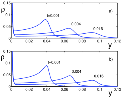
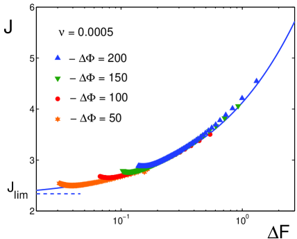
Figure 1: (Left) Distribution of the charge density $\rho$ in space for several moments of time, $\Delta V=100$ and $\nu=\tilde{\lambda_{D}}/\tilde{L}=0.001$; (a) — numerical solution of (1)–(3), (b) — self-similar solution. The numerical points for $\nu=0.0005$, and several values of $\Delta V$ shrink into one self-similar VC curve (shown by the solid line).

The self-similar rescaling of the variables, along with the 1D assumption, turns the PDE system (1)–(2) into the ODE system with the new dimensionless spatial variable $\eta=\tilde{y}/\sqrt{4{\tilde{D}\tilde{t}}}$ and a small parameter $\varepsilon=\tilde{\lambda}_{D}/\sqrt{4{\tilde{D}\tilde{t}}}$. A new dimensionless Debye length $\varepsilon$, electric current $J$ and drop of potential $\Delta\Phi$ in self-similar variables are connected with the corresponding old variables, $\nu$, $j$ and $\Delta V$, by the relations

$$\varepsilon(t)=\frac{\nu}{2\sqrt{t}},\quad J(t)=2j(t)\sqrt{t},\quad\Delta\Phi(t)=\Delta V-\frac{j(t)}{2}.$$ (4)

The two-parameter family of self-similar solutions for the parameters $\Delta\Phi$ and $\varepsilon$ is found in [9, 10, 11] and now is compared with the DNS of (1)–(3). In Fig. 1 (left), such a comparison for the charge distribution $\rho(\eta){\,=\,c^{+}(\eta)\,-\,}c^{-}(\eta)$ is presented for different moments of time where the parameters of the self-similar solutions are recalculated according to (4). In Fig. 1 (right) universal voltage–current characteristics $J$ versus $\Delta F=\varepsilon\Delta\Phi$ are shown by a solid line while triangles, stars and circles are gathered for several fixed drops of potential between the membranes, $\Delta V$, for intermediate times. The numerical points for all $\Delta V$ shrink into the universal self-similar VC curve. A rather good correspondence justifies a self-similar behavior at intermediate times.

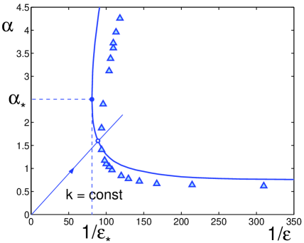
Figure 2: Marginal stability curve at $\Delta V=40$ and $\nu=0.001$. The time-dependent coordinates are inverse Debye length $1/\varepsilon$ and wave number $\alpha$. Each straight line corresponds to a perturbation with a given wave number $k$; a point on the line is moving with time towards the stability curve and eventually crosses it.

Figure 3: Wave number selection for the room disturbances; darker regions correspond to larger amplitudes. Broadband initial noise is transformed into a sharp band near $k\approx 32\div 34$, dashed line corresponds to the prediction of stability theory, $k_{*}=35$, $\Delta V=50$ and $\nu=0.001$.

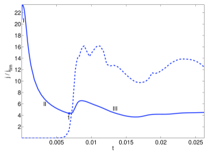
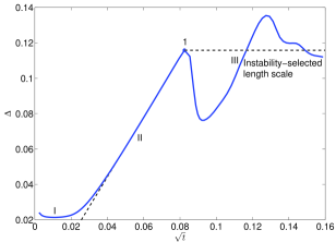
Figure 4: Typical evolution of the average electric current $\langle j\rangle/j_{\lim}$ (solid line) and current amplitude $j_{\max}-j_{\min}$ (dashed line) (left) and diffusion layer thickness (right) from room disturbances for $\nu=0.001$ and $\Delta V=60$. Three time intervals are exhibited; point 1 specifies the instability selected length scale.

Instability of the self-similar solution and the length scale selection. The initial stage of evolution is one-dimensional and self-similar, but room disturbances (3) for the super-critical case, $\Delta V>\Delta V_{*}$, will grow and eventually manifest themselves, destroying the self-similarity and making the solution two-dimensional. This specifies the next step of evolution. When the amplitudes of the harmonics are small, their behavior can be considered independently. Imposing on the 1D self-similar solution a perturbation of the form $\hat{R}(\eta,t)\exp{(i\alpha x)}$ and linearizing (1)–(3) with respect to $\hat{R}$ turns this system into a linear PDE system with time-dependent coefficients. Restricting ourselves to neutral perturbations, $\partial/\partial t=0$, transforms this PDE system into an ODE system in $\eta$. Solution of the eigenvalue problem for this system gives the marginal stability conditions [9].

The parametric dependence of the Debye length and wave number for the self-similar solution in time completely changes the interpretation of the marginal stability curves [11]. It is instructive to present the stability curve at a fixed drop of potential $\Delta V$ in coordinates of the inverse Debye length $1/\varepsilon=2\sqrt{t}/\nu$ versus the wave number $\alpha=k\nu/\varepsilon=2k\sqrt{t}$, both referred to the self-similar length $\sqrt{4\tilde{D}\tilde{t}}$ and, so, time-dependent, see Fig. 2. Each straight line in the figure corresponds to a monochromatic wave with a fixed wave number, $k=\tilde{\alpha}\tilde{L}$; the larger is $k$, the steeper is the line. Inside the marginal stability curve a perturbation is growing, but outside — decaying. A point on the straight line corresponding to some initial perturbation is moving with time towards the marginal stability curve just because of the parametrical time dependence of axes. At the same time, the amplitude of the disturbance at the beginning is always decaying but after crossing the marginal curve at some point, it starts to grow. The nose critical point with coordinates $(1/\varepsilon_{*},\alpha_{*})$ first reaches the marginal stability curve and, hence, first loses its stability. Triangles in the figure are taken from our DNS for monochromatic perturbations. There is a rather good quantitative agreement between the numerical simulations and the stability theory for self-similar solutions.

Room disturbances at the linear stage of evolution can be considered as a superposition of individual harmonics. Their evolution always starts in the stable region and filters a broadband initial noise (3) into a sharp band of wave numbers. It stands to reason that we may assume that the wave number selection is determined by the critical points $(1/\varepsilon_{*},\alpha_{*})$ with the characteristic wave number $k_{*}=\alpha_{*}\varepsilon_{*}/\nu$. This principle is different from the well-known selecting principle of maximum growing mode and is verified by comparison of the results of the DNS with the BC’s (3): the comparison for typical conditions presented in Fig. 3 shows the validity of this novel principle.

The relation $\Delta(t)=2/\langle j(t)\rangle$ between the diffusion layer thickness $\Delta$ and the electric current averaged along the membrane length $l$, $\langle j\rangle=\frac{1}{l}\int_{0}^{l}j(x,t)dx$, is accepted. For the self-similar solution the diffusion layer thickness should be proportional to the square root of time, $\Delta(t)\sim\sqrt{t}$, and, respectively, $\langle j(t)\rangle\sim 1/\sqrt{(}t)$. The typical evolution of the electric current $\langle j\rangle$ and of the diffusion layer thickness $\Delta$, presented in Fig. 4, exhibit three characteristic time intervals. In the interval II, for times of intermediate magnitude, $\Delta$ is proportional to $\sqrt{t}$ and the behavior is one-dimensional and self-similar, while for shorter times, in the time interval I, as well as for longer times in the interval III, this self-similarity is violated. In region I, the influence of the initial conditions is important, while in region III, the growth of $\Delta$ is arrested by instability. The current amplitude $j_{\max}-j_{\min}$ characterizes instability and is shown by the dashed line in Fig. 4 (left); it becomes significant at the point $1$ which separates regions II and III and specifies the characteristic length of the diffusion layer. Further calculations show that this length selected by instability is not changed much by subsequent nonlinear processes.

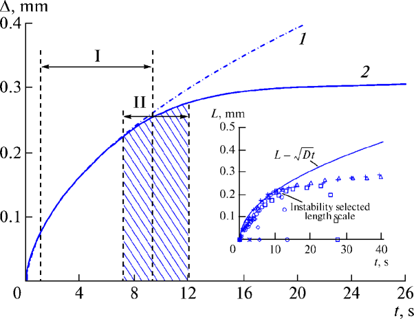
Figure 5: Time dependence of the thickness of the diffusion layer $\tilde{\Delta}$ in dimensional variables for $\Delta\tilde{V}=2.5$ V, $\tilde{L}=1$ mm, $\tilde{D}=5\cdot 10^{-9}$ $\mbox{m}^{2}/\mbox{s}$ and $\nu=0.001$ [10]. (1) Self-similar solution, (2) numerical solution, I is the self-similarity range, and II is the stability loss by the trivial solution and the appearance of electroconvection. The corresponding experimental dependence [7] is in the inset.

In Fig. 5, a qualitative comparison with the experiments of Yossifon and Chang [7] is presented (for details see [10]). The time dependence of the thickness of the diffusion layer $\tilde{\Delta}$ is taken in dimensional variables. Excluding very short times of establishment, up to $8.9$ s of evolution, the solution in zone I follows the self-similar law proportionally to $\sqrt{\tilde{t}}$ (dash-and-dot line); then the self-similar process is violated by the loss of stability in zone II. According to the numerical experiment, the transition to the electroconvection mode takes place in the range $6\div 10$ s. This corresponds to the value of 8 s observed in physical experiments [7].

Nonlinear stages of evolution and secondary instability. The next stages of evolution are nonlinear processes with eventual saturation of the disturbance amplitude. For a small super-criticality, $\Delta V-\Delta V_{*}$, the nonlinear saturation leads to steady periodic electro-convective vortices along the membrane surface; with increasing super-criticality the attractor can be described as a structure of periodically oscillating vortices; with further increase in super-criticality, the behavior eventually becomes chaotic in time and space.

The evolution of the normalized to $j_{\lim}$ average electric current and current amplitude of perturbation are presented in Fig. 6. For small super-criticality this evolution results in steady vortices, Fig. 6 (left), and for larger super-criticality — in chaotic behavior, Fig. 6 (right).

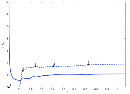
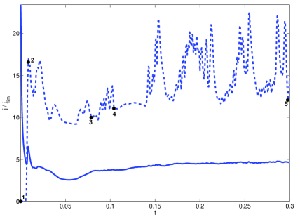
Figure 6: Evolution of the normalized average electric current $\langle j\rangle/j_{\lim}$ (solid line) and current amplitude $(j_{\max}-j_{\min})/j_{\lim}$ (dashed line) for $\nu=0.001$ $\kappa=0.2$ for small super-criticality, $\Delta V=30$ (left) and for large super-criticality, $\Delta V=50$ (right).

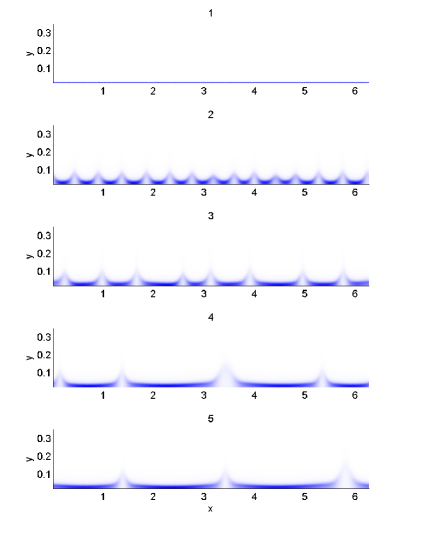
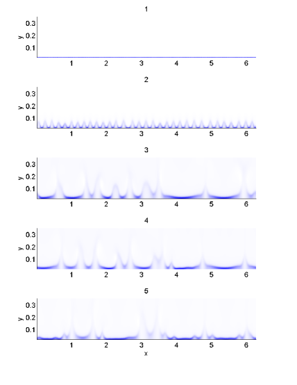
Figure 7: Snapshots of the charge density $\rho(x,y,t)$ at different times. Darker regions correspond to larger charge densities (for parameters, see previous figure).

Snapshots of the charge density $\rho(x,y,t)$ for the above mentioned conditions at different times are shown in Fig. 7. Darker regions correspond to larger densities of space charge. There is a rather sharp boundary between the ESC region and the diffusion region. Point 1 corresponds to the initial small-amplitude broadbanded white noise. A linear stability mechanism filters it into practically periodic disturbances with a wave number $k_{*}$, point 2. The boundary between the ESC region and the diffusion region behaves sinusoidally: its minimum corresponds to the maximum of the charge density and vice versa. With increasing time, there is a fusion of neighboring waves with corresponding reducing of their number. The sinusoidal profile changes to the spike-like one where regions of small charge in the spikes are jointed by thin flat regions of large space charge, moment 5, left. Besides fusion of the spikes there is also their creation so that eventually some equilibrium of their number is established, moment 5, right. Movie visualization for charge density evolution can be found in [13] ($\Delta V=50$, $\nu=10^{-3}$ and $\kappa=0.2$, chaotic behavior).

Let us consider the physical mechanisms of the secondary instability. The sharp boundary between the ESC and diffusion regions has small charge densities near its humps and large charge densities in neighboring regions around its hollows, either for periodic or spike-like coherent structures. These regions with larger charge are trying to expand (charge of the same sign is repelling) and this can lead to the disappearance of some of the humps — with eventual coarsening. Such instability is illustrated in Fig. 8 (left). There is also another physical mechanism which results in the opposite effect. If a flat region between two humps is long enough, it suffers from primary Rubinstein and Zaltsman electroconvective instability, see Fig. 8 (right). Points 1, 2 and 3 are nucleation points of future humps. They grow and eventually form new humps. This last mechanism is applicable only for spike-like structures with flat neighboring regions, but not for sinusoidal waves.

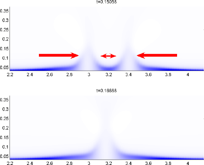
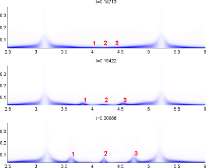
Figure 8: Two physical mechanisms of the secondary instability. (a) Coalescence of two humps with low charge density with following coarsening. (b) Instability of flat region between humps with following creation of new humps.

Conclusions. The results of the DNS reported in this paper refer to realistic experimental parameters that may be realized in lab experiments. The following stages of evolution are identifed: i) a stage in which the initial conditions have considerable influence (milliseconds); ii) 1D self-similar evolution (milliseconds–seconds); iii) primary instability of the self-similar solution (seconds); iv) a nonlinear stage with secondary instabilities. This work can be viewed as a new step in the understanding of the instabilities and pattern formation in micro- and nano-scales.

The authors are grateful to I. Rubinstein, M. Z. Bazant, and H.- C. Chang for fruitful discussions. This work was supported in part by Russian Foundation for Basic Research (project no. 11-08-00480-a).

Figure Captions

• (Left) Distribution of the charge density $\rho$ in space for several moments of time, $\Delta V=100$ and $\nu=\tilde{\lambda_{D}}/\tilde{L}=0.001$; (a) — numerical solution of (1)–(3), (b) — self-similar solution. The numerical points for $\nu=0.0005$, and several values of $\Delta V$ shrink into one self-similar VC curve (shown by the solid line).

• Marginal stability curve at $\Delta V=40$ and $\nu=0.001$. The time-dependent coordinates are inverse Debye length $1/\varepsilon$ and wave number $\alpha$. Each straight line corresponds to a perturbation with a given wave number $k$; a point on the line is moving with time towards the stability curve and eventually crosses it.

• Wave number selection for the room disturbances; darker regions correspond to larger amplitudes. Broadband initial noise is transformed into a sharp band near $k\approx 32\div 34$, dashed line corresponds to the prediction of stability theory, $k_{*}=35$, $\Delta V=50$ and $\nu=0.001$.

• Typical evolution of the average electric current $\langle j\rangle/j_{\lim}$ (solid line) and current amplitude $j_{\max}-j_{\min}$ (dashed line) (left) and diffusion layer thickness (right) from room disturbances for $\nu=0.001$ and $\Delta V=60$. Three time intervals are exhibited; point 1 specifies the instability selected length scale.

• Time dependence of the thickness of the diffusion layer $\tilde{\Delta}$ in dimensional variables for $\Delta\tilde{V}=2.5$ V, $\tilde{L}=1$ mm, $\tilde{D}=5\cdot 10^{-9}$ $\mbox{m}^{2}/\mbox{s}$ and $\nu=0.001$ [10]. (1) Self-similar solution, (2) numerical solution, I is the self-similarity range, and II is the stability loss by the trivial solution and the appearance of electroconvection. The corresponding experimental dependence [7] is in the inset.

• Evolution of the normalized average electric current $\langle j\rangle/j_{\lim}$ (solid line) and current amplitude $(j_{\max}-j_{\min})/j_{\lim}$ (dashed line) for $\nu=0.001$ $\kappa=0.2$ for small super-criticality, $\Delta V=30$ (left) and for large super-criticality, $\Delta V=50$ (right).

• Snapshots of the charge density $\rho(x,y,t)$ at different times. Darker regions correspond to larger charge densities (for parameters, see previous figure).

• Two physical mechanisms of the secondary instability. (a) Coalescence of two humps with low charge density with following coarsening. (b) Instability of flat region between humps with following creation of new humps.

References

- [1] M. C. Cross and P. G. Hohenberg, Rev. Modern Physics 65, 3, 851 (1993).
- [2] I. Rubinstein, and B. Zaltzman, Phys. Rev. E 62, 2238 (2000); I. Rubinstein, and B. Zaltzman, Phys. Rev. E 68, 032501 (2003); I. Rubinstein, B. Zaltzman, and I. Lerman, Phys. Rev. 72, 011505 (2005).
- [3] B. Zaltzman and I. Rubinstein, J. Fluid Mech. 579, 173 (2007).
- [4] I. Rubinstein, E. Staude, and O. Kedem, Desalination 69, 101 (1988); F. Maletzki, H. W. Rossler, and E. Staude, J. Membr. Sci. 71, 105 (1992); I. Rubinstein, B. Zaltzman, J. Pretz, and C. Linder, Rus. J. Electrochem. 38, 853 (2004); E. I. Belova, G. Lopatkova, N. D. Pismenskaya, V. V. Nikonenko, C. Larchet, and G. Pourcelly, J. Phys. Chem. B 110, 13458 (2006).
- [5] S. M. Rubinstein, G. Manukyan, A. Staicu, I. Rubinstein, B. Zaltzman, R. G. H. Lammertink, F. Mugele, and M. Wessling, Phys. Rev. Lett. 101, 236101 (2008).
- [6] S. J. Kim, Y.-C. Wang, J. H. Lee, H. Jang, and J. Han, Phys. Rev. Lett. 99, 044501.1 (2007).
- [7] G. Yossifon and H.-C. Chang, Phys. Rev. Lett. 101, 254501 (2008).
- [8] E. A. Demekhin, V. S. Shelistov, and N. V. Nikitin, Phys. Fluids (in preparation).
- [9] E. A. Demekhin, E. M. Shapar, and V. V. Lapchenko, Doklady Physics 53, 450 (2008).
- [10] E. N. Kalaidin, S. V. Polyanskikh, and E. A. Demekhin, Doklady Physics 55, 502 (2010).
- [11] E. A. Demekhin, S. V. Polyanskikh, and Y. M. Shtemler, Submitted to Phys. Fluids.
- [12] J. P. Gollub and H. L. Swinney, Phys. Rev. Letters, 35, 921 (1975).
- [13] http://demekhin.kubannet.ru/electrokinetic.php