Aharonov-Bohm-Coulomb Problem in Graphene Ring

Abstract

We study the Aharonov-Bohm-Coulomb problem in a graphene ring. We investigate, in particular, the effects of a Coulomb type potential of the form $\xi/r$ on the energy spectrum of Dirac electrons in the graphene ring in two different ways: one for the scalar coupling and the other for the vector coupling. It is found that, since the potential in the scalar coupling breaks the time-reversal symmetry between the two valleys as well as the effective time-reversal symmetry in a single valley, the energy spectrum of one valley is separated from that of the other valley, demonstrating a valley polarization. In the vector coupling, however, the potential does not break either of the two symmetries and its effect appears only as an additive constant to the spectrum of Aharonov-Bohm potential. The corresponding persistent currents, the observable quantities of the symmetry-breaking energy spectra, are shown to be asymmetric about zero magnetic flux in the scalar coupling, while symmetric in the vector coupling.

1 Introduction

Graphene is a two-dimensional composite lattice with honeycomb structure and consists of two sublattices of carbon atoms. The corresponding Brillouin zone (BZ) is also a hexagon with high symmetry points at vertices as well as center and side (see Fig. 1) [1, 2]. Near the vertices of the BZ the low-energy electronic spectra are linearly dependent on the magnitude of momentum, forming conical valleys, and the dynamics of electrons in graphene can be formulated by Dirac equation of massless fermion [3, 4]. Because of this Dirac fermion-like behavior of electrons, graphene may offer an opportunity to test the various predictions of the planar field theories [5, 6] by experiment with solid state material. In this respect there have been much effort to connect the two-dimensional (2D) field theory with the graphene physics [7], including the Aharonov-Bohm (AB) effect [8] in a ring geometry of graphene [9, 10, 11, 12].

The studies of the AB effect in a graphene ring were mostly concerned about the breaking of time-reversal symmetry (TRS) that yields a splitting of the valley degeneracy due to the time-reversal symmetry in graphene. In this regard, the authors of Ref. [9] have demonstrated that the splitting of the degeneracy in a single valley can be controlled by the threaded magnetic flux and a confinement potential of the Dirac electrons on the AB ring of graphene. An interesting result from the work was that the confinement potential, introduced as a mass term in the Dirac equation, leads to a breaking of the TRS in the absence of the magnetic flux.

In this paper, motivated from the above result, we study the Aharonov-Bohm-Coulomb (ABC) problem [13, 14] in a graphene ring to investigate the effect of a Coulomb type potential in the form of $\xi/r$ on the splitting of valley degeneracy.  Within the framework of field theory there are many possible ways in introducing the potential to the Dirac equation. The only criterion for a consistent coupling of the potential to the Dirac equation is the fact that the larger component of the Dirac field $\varphi$ should satisfy the Schrödinger equation $\left[p^{2}/2M+\xi/r\right]\varphi=\mathcal{E}\varphi$ in the non-relativistic Galilean limit [15]. In fact, there are at least two ways such that the same consistent Galilean limit is fulfilled. In the present work we consider the following two possibilities [16]: one is the scalar coupling and the other is the vector coupling. As we shall describe explicitly in next section, in the former case the $\xi/r$ potential enters the Dirac equation as a mass term, while it enters the equation as an energy term in the latter case. From the viewpoint of time-reversal symmetry the scalar coupling is expected to break the TRS, but the vector coupling is not. In the following, we explicitly show that the scalar coupling indeed leads to the splitting of valley degeneracy, while the vector coupling does not. What is remarkable and new in our result is that, besides the splitting of the single-valley degeneracy, the scalar coupling produces a separation between the energy spectrum of one valley and that of the other valley, and the separation increases with the interaction strength $\xi$.

The paper is organized as follows. In Sec. 2, starting with a brief recapitulation of the time-reversal symmetries in graphene, we give a qualitative argument how the TRS is broken by the $\xi/r$ potential in the AB ring of graphene, whereby the splitting of valley degeneracy is produced. In Sec. 3 we solve the 2D Dirac equation for the scalar coupling of the potential in a graphene ring. We derive an analytical expression of the energy spectrum in terms of valley parameter (denoted by $\tau$) and the interaction strength $\xi$. These two parameters interplay to separate the whole energy spectrum of one valley from the other. We then compute a persistent current in the ring. Owing to the separation of energy spectra the persistent current is asymmetric about the zero magnetic flux, which represents an essentially single-valley characteristic in the case of scalar coupling, known as the valley polarization [17, 18]. In Sec. 4, we present the energy spectrum for the vector coupling. It is shown that, contrary to the scalar coupling case, the potential via vector coupling to the Dirac equation alone can break neither the intravalley nor the intervalley degeneracies because of the conservation of the TRS. We find that the potential in the vector coupling serves effectively as an additive constant in the energy spectrum and is completely decoupled from the AB effect. Finally, there will be a conclusion in Sec. 5.

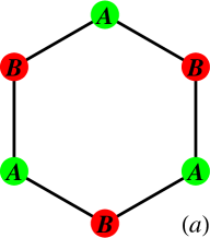
Figure 1: The Honeycomb lattice (left) consists of two sublattices, one with $A$ atoms and the other with $B$ atoms. The right is the corresponding Brillouin zone and its symmetry points. Note that the two symmetry points, $\bm{K}$ and $\bm{K^{\prime}}$, are related by $\bm{K^{\prime}}=-\bm{K}$. The energy spectra near these points for conduction band are given by $E=\hbar v_{F}|\bm{k}\pm\bm{K}|$, which are the conic dispersion relations, called valleys.

2 TRS breaking and splitting of valley degeneracy

In this section we first briefly recapitulate the discrete symmetry of the time reversal in graphene, then discuss the symmetry breaking in the ABC problem of graphene ring. As illustrated in Fig. 1 there are two inequivalent symmetry points $\bm{K}$ and $\bm{K^{\prime}}$ in the BZ of a graphene, and to each point two sublattices $A$ and $B$ are associated. The Hamiltonian of a Dirac electron in graphene is conveniently described by two pseudospins related to the two valleys at $\bm{K}$ and $\bm{K^{\prime}}$ and the two sublattices. In the following we use the Pauli matrices $\bm{\tau}=(\tau_{1},\tau_{2},\tau_{3})$ and $\bm{\sigma}=(\sigma_{1},\sigma_{2},\sigma_{3})$ to denote the valley and sublattice degree of freedom, respectively and also use the $2\times 2$ unit matrices $\tau_{0}$ and $\sigma_{0}$. Based on the geometry in Fig. 1 the Hamiltonian and corresponding four-component spinor can be described as

$$\displaystyle H_{0}=\tau_{0}\otimes H_{K},\quad H_{K}=v_{F}\bm{\sigma}\cdot\mathbf{p},\quad\Psi=(\Psi_{AK},\Psi_{BK},-\Psi_{BK^{\prime}},\Psi_{AK^{\prime}})^{T},$$ (1)

where $v_{F}\sim c/300$ is the Fermi velocity, $T$ stands for transpose, and we have used the valley-isotropic form of hamiltonian for convenience of subsequent calculations [17].

To see the TRS in graphene we introduce the following time-reversal operator

$$\displaystyle\eqalign{\mathcal{T}=\left[(i\tau_{2})\otimes(i\sigma_{2})\right]\mathcal{C},}$$ (3)

where $\mathcal{C}$ is the complex conjugate operator. The effect of $\mathcal{T}$ on the Hamiltonian $H_{0}$ and the state $\Psi$ are

$$\displaystyle\eqalign{\mathcal{T}H_{0}\mathcal{T}^{-1}=H_{0},\quad\mathcal{T}\Psi=(\Psi_{AK^{\prime}}^{*},\Psi_{BK^{\prime}}^{*},-\Psi_{BK}^{*},\Psi_{AK}^{*})^{T}.}$$ (5)

This shows that the Hamiltonian $H_{0}$ is invariant under the transformation by $\mathcal{T}$ but it interchanges the valleys; there exists a degeneracy between the two valleys (henceforth, intervalley degeneracy). According to Ref. [19], the Hamiltonian satisfies another TRS under the transformation by the operator

$$\displaystyle\eqalign{\bm{\Theta}=\tau_{0}\otimes\bm{\Theta}_{\sigma},\quad\bm{\Theta}_{\sigma}=i\sigma_{2}\mathcal{C}.}$$ (7)

With this operator one can verify

$$\displaystyle\eqalign{\bm{\Theta}H_{0}{\bm{\Theta}}^{-1}=H_{0},\quad\bm{\Theta}\Psi=(\Psi_{BK}^{*},-\Psi_{AK}^{*},\Psi_{AK^{\prime}}^{*},\Psi_{BK^{\prime}}^{*})^{T}.}$$ (9)

This operator exchanges the sublattices within a single valley, but does not interchange the valleys as we can see in the right equation. Since the Hamiltonian $H_{0}$ is invariant this leads to a degeneracy within a single valley (henceforth, intravalley degeneracy) [20]. More specifically, the operator $\bm{\Theta}_{\sigma}$ transforms $H_{K}$ in Eq. (1) to $\bm{\Theta}_{\sigma}H_{K}\bm{\Theta}_{\sigma}^{-1}=H_{K}$, that is, $H_{K}$ is invariant as the intravalley degeneracy implies: $\bm{\Theta}_{\sigma}$ effectively changes the sign of $\bm{\sigma}$ and $\mathbf{p}$.

Having introduced the TRS’s of graphene we now discuss the TRS breaking of the ABC problem in a graphene ring. For this we first consider an AB type ring of a graphene discussed in Ref. [9]: inner and outer radii of the ring are $a+w/2$ and $a-w/2$, so that the ring width is $w$. Since the Hamiltonian $H_{0}$ has a valley-isotropic form it is more convenient to use $H_{K}$ with two-component spinor and insert the valley index in an appropriate place. For the AB ring the Hamiltonian then reads 

$$\displaystyle H(\bm{A})=H_{K}(\bm{A})+\tau V(r)\sigma_{3},\quad H_{K}(\bm{A})=v_{F}\bm{\sigma}\cdot\left(\bm{p}+e\bm{A}\right)$$ (10)

where the circularly symmetric potential $\tau V(r)\sigma_{3}$ is introduced to confine a Dirac electron on the graphene ring: $V(r)=0$ when $|r-a|\leq w/2$ and $V(r)\rightarrow\infty$ when $|r-a|\geq w/2$. The index $\tau=\pm 1$ denotes the valleys: $\tau=+1$ for the $\bm{K}$ valley and $\tau=-1$ for the $\bm{K^{\prime}}$ valley. We note here that this potential is proportional to $\sigma_{3}$.

Obviously the magnetic field breaks the effective TRS of $\bm{\Theta}_{\sigma}$: ${\bm{\Theta}}_{\sigma}H_{K}({\bm{A}}){\bm{\Theta}}_{\sigma}^{-1}=H_{K}(-{\bm{A}})$. In fact, the TRS of the Hamiltonian with four-component spinor is also broken: $\mathcal{T}[\tau_{0}\otimes H_{K}({\bm{A}})]\mathcal{T}^{-1}=\tau_{0}\otimes H_{K}({-\bm{A}})$. Thus, the presence of magnetic field will lift both of the intervalley and intravalley degeneracies. What is interesting in Eq. (10) is the TRS breaking by the confinement potential term when $\bm{A}=0$. In the absence of magnetic field one can see

$$\displaystyle\eqalign{\bm{\Theta}_{\sigma}[H_{K}(0)+\tau V(r)\sigma_{3}]\bm{\Theta}_{\sigma}^{-1}=H_{K}(0)-\tau V(r)\sigma_{3}.}$$ (12)

This implies the intervalley degeneracy can be broken by the confinement potential as demonstrated in Ref. [9]. According to Berry [21] this potential enters the 2-D Dirac equation by the replacement of $Mc^{2}\rightarrow Mc^{2}+V(r)\sigma_{3}$ with $M=0$ for a massless particle. In this sense the confinement potential is regarded as a mass term in the Dirac equation, and it can be conjectured that a mass term proportional to $\sigma_{3}$ leads to a breaking of the effective TRS in an AB graphene ring.

We now turn to the problem of ABC in a graphene ring. Here we need to include a Coulomb type potential $\xi/r$ in the Dirac equation. To address the TRS breaking by this potential we begin with the general form of a 2D relativistic Dirac equation minimally coupled to AB potential $\bm{A}$, which can be written as

$$\eqalign{\left[c\beta{\boldmath\gamma}\cdot{\boldmath\Pi}+\beta Mc^{2}\right]\psi=E\psi,}$$ (13)

where $M$ is the bare mass of a Dirac electron, $\psi$ is the two-component spinor, and $\Pi_{i}=-i\partial_{i}-eA_{i}$ is the covariant derivative multiplied by $-i$. The Dirac matrix is chosen as

$$\eqalign{\beta=\sigma_{3},\quad\beta\gamma_{i}=(\sigma_{1},s\sigma_{2}),\quad\{\gamma^{\mu},\gamma^{\nu}\}=2\eta^{\mu\nu},\quad\eta^{\mu\nu}=(+,-,-),}$$ (15)

where $s$ is twice of the spin value ($+1$ for spin “up” and $-1$ for spin “down”). We employ a thin flux tube as the AB potential in the form

$$eA_{i}=\frac{\alpha\epsilon_{ij}r_{j}}{r^{2}},$$ (16)

which yields the magnetic field $B=-2\pi\alpha\delta({\boldmath r})/e$ along the $z$-direction as expected. Therefore, the parameter $\alpha$ represents a magnetic flux in unit of $-e/(2\pi)$.

As mentioned in introduction there are at least two possibilities for the potential $\xi/r$  to be included in the Dirac equation, the scalar coupling and the vector coupling. For the scalar coupling it couples to the equation as

$$\displaystyle\eqalign{\left[c\beta{\boldmath\gamma}\cdot{\boldmath\Pi}+\beta\left(Mc^{2}+\frac{\xi}{r}\right)\right]\psi=E\psi,}$$ (18)

and for the vector coupling the equation becomes

$$\displaystyle\eqalign{\left[c\beta{\boldmath\gamma}\cdot{\boldmath\Pi}+\beta Mc^{2}\right]\psi=\left(E-\frac{\xi}{r}\right)\psi.}$$ (20)

From a physical point of view the potential $\xi/r$ in the vector coupling corresponds to the electric Coulomb potential (time component of the relativistic four vector) and the potential in the scalar coupling is a relativistic scalar potential (other than the electric Coulomb potential). For the Dirac electron in a graphene, since $M=0$ and $c=v_{F}$, we have

$$H_{s}\psi=E\psi,\quad H_{s}(\bm{A})=H_{K}(\bm{A})+\frac{\xi}{r}\sigma_{3},$$ (21)

$$H_{v}\psi=E\psi,\quad H_{v}(\bm{A})=H_{K}(\bm{A})+\frac{\xi}{r},$$ (22)

where $H_{s}(\bm{A})$ and $H_{v}(\bm{A})$ stand for Hamiltonians of scalar coupling and vector coupling, respectively, $H_{K}(\bm{A})$ is given in Eq. (10), and we have used the conventions in Eq. (15) with $s=+1$.

As before the magnetic field will break both of the TRS’s for $\mathcal{T}$ and $\bm{\Theta}$. To see the effect of the potential $\xi/r$, we take the time-reversal transformation on the Hamiltonians for $\bm{A}=0$. For the operator $\mathcal{T}$ we get

$$\displaystyle\eqalign{\mathcal{T}\tau_{0}\otimes H_{s}(0)\mathcal{T}^{-1}=\tau_{0}\otimes\left[H_{K}(0)-\frac{\xi}{r}\sigma_{3}\right],\cr\displaystyle\mathcal{T}\tau_{0}\otimes H_{v}(0)\mathcal{T}^{-1}=\tau_{0}\otimes\left[H_{K}(0)+\frac{\xi}{r}\right].}$$ (25)

The scalar coupling breaks the TRS for $\mathcal{T}$, but the vector coupling preserves the TRS. For the effective TRS operator $\bm{\Theta}_{\sigma}$ the two Hamiltonians are transformed to

$$\displaystyle\eqalign{\bm{\Theta}_{\sigma}H_{s}(0)\bm{\Theta}_{\sigma}^{-1}=H_{K}(0)-\frac{\xi}{r}\sigma_{3},\cr\displaystyle\bm{\Theta}_{\sigma}H_{v}(0)\bm{\Theta}_{\sigma}^{-1}=H_{K}(0)+\frac{\xi}{r}.}$$ (28)

Here we have the same results: the scalar coupling breaks the effective TRS for $\bm{\Theta}_{\sigma}$, but the vector coupling does not. Therefore we expect that the scalar coupling will lift both of the intervalley and intravalley degeneracies. On the other hand, the vector coupling breaks neither of the two degeneracies. In the following sections we will compute the energy spectra of the ABC problem in a graphene ring to show the effects of each coupling explicitly.

3 ABC problem with scalar coupling

In this section we compute the energy spectrum for the scalar coupling of ABC in a graphene ring. As described before the geometry of the ring is the same as discussed in Ref. [9]. Using the Hamiltonian (21) and the confinement potential in Eq. (10) the 2D Dirac equation is

$$H_{s}\psi=E\psi,\quad H_{s}=\left[v_{F}\bm{\sigma}\cdot\left(\bm{p}+e\bm{A}\right)+\frac{\xi}{r}\sigma_{3}\right]+\tau V(r)\sigma_{3},$$ (29)

where $\tau=\pm$ is the valley index. As defined earlier, in the confinement potential, $V(r)=0$ when $|r-a|\leq w/2$ and $V(r)\rightarrow\infty$ when $|r-a|>w/2$. According to Refs. [21] and [22] the boundary conditions on the two-component spinor $\psi$ can be expressed as the form

$$\displaystyle\psi=\tau({\bm{n}}_{\perp}\cdot{\bm{\sigma}})\psi,\quad\left\{\begin{array}[]{ll}{\bm{n}}_{\perp}=(-\sin\theta,\,\cos\theta),&~{}r=a+\frac{w}{2}\\ {\bm{n}}_{\perp}=-(-\sin\theta,\,\cos\theta),&~{}r=a-\frac{w}{2}\end{array}\right.$$ (32)

where ${\bm{n}}_{\perp}$ is the unit vector perpendicular to the normal direction ${\bm{n}}$ on the boundary (i.e, ${\bm{n}}_{\perp}\cdot{\bm{n}}=0$) and lies in $(x,y)$ plane, that is, on the ring plane. This choice of boundary conditions is based on the requirement of the hermiticity of the Hamiltonian $H$ within the boundary, which yields the condition of no outward current at any point on the ring boundary (i.e., ${\bm{n}}\cdot{\bm{v}}=0$, where ${\bm{v}}=<\psi|v_{F}{\bm{\sigma}}|\psi>$). 

For a Dirac electron inside the ring the Dirac equation reads, using $V(r)=0$,

$$\left[{\bm{\sigma}}\cdot\left(\bm{p}+e\bm{A}\right)+\frac{\tilde{\xi}}{r}\sigma_{3}\right]\psi=\tilde{E}\psi$$ (33)

where $\tilde{E}=E/v_{F}$ and $\tilde{\xi}=\xi/v_{F}$. Operating $[-{\bm{\sigma}}\cdot\left(\bm{p}+e\bm{A}\right)+\sigma_{3}\tilde{\xi}/r+\tilde{E}]$ on the equation and using polar coordinates we have second order equations

$$\eqalign{\left[\partial_{r}^{2}+\frac{1}{r}\partial_{r}+\frac{1}{r^{2}}\left(\partial_{\theta}+i\alpha\right)^{2}-\frac{\tilde{\xi}^{2}}{r^{2}}+\tilde{E}^{2}+seB\sigma_{3}\right]\psi\cr=\frac{i\tilde{\xi}}{r^{2}}\left(\begin{array}[]{cc}0&-e^{-is\theta}\\ e^{is\theta}&0\end{array}\right)\psi,}$$ (38)

where $B$ and $\alpha$ are the magnetic field and flux given in Eq. (16). Since the Hamiltonian (29) satisfies $[H,J_{3}]=0$, where $J_{3}=-i\partial_{\theta}+(s/2)\sigma_{3}$, the solution to the Dirac equation can be written in the form

$$\psi(r,\theta)=\left(\begin{array}[]{c}\chi_{1m}(r)e^{i(m-s/2)\theta}\\ \chi_{2m}(r)e^{i(m+s/2)\theta}\end{array}\right),\quad\left(m=\pm\frac{1}{2},\pm\frac{3}{2},\cdots\right).$$ (41)

Inserting this into Eq. (38) we can extract the radial equation

$$\eqalign{\left[\partial_{r}^{2}+\frac{1}{r}\partial_{r}-\frac{(m+\alpha)^{2}+\tilde{\xi}^{2}+1/4}{r^{2}}+\tilde{E}^{2}\right]\left(\begin{array}[]{c}\chi_{1m}(r)\\ \chi_{2m}(r)\end{array}\right)\cr=-\frac{1}{r^{2}}(\eta\sigma_{3}-\tilde{\xi}\sigma_{2})\left(\begin{array}[]{c}\chi_{1m}(r)\\ \chi_{2m}(r)\end{array}\right)},$$ (48)

where

$$\eta=m+\alpha.$$ (49)

Using the matrix diagonalization the right hand side can be written as

$$\displaystyle\eqalign{\eta\sigma_{3}-\tilde{\xi}\sigma_{2}=\epsilon(\eta)\sqrt{\eta^{2}+\tilde{\xi}^{2}}\,U_{c}^{\dagger}\sigma_{3}U_{c}\cr U_{c}=\cos\frac{\phi}{2}\sigma_{0}+i\sin\frac{\phi}{2}\sigma_{1}\quad\left(-\frac{\pi}{2}\leq\phi=\tan^{-1}\frac{\tilde{\xi}}{\eta}\leq\frac{\pi}{2}\right)},$$ (52)

where $\epsilon(x)=|x|/x$ is the alternating function, $\sigma_{0}$ is the $2\times 2$ unit matrix, and

$$\tan\frac{\phi}{2}=\epsilon(\eta)\frac{\sqrt{\eta^{2}+\tilde{\xi}^{2}}-|\eta|}{\tilde{\xi}}.$$ (53)

With this diagonalization the radial equation (48) reduces to

$$\eqalign{\left[\partial_{r}^{2}+\frac{1}{r}\partial_{r}-\frac{(m+\alpha)^{2}+\tilde{\xi}^{2}+1/4}{r^{2}}+\tilde{E}^{2}\right]\left(\begin{array}[]{c}f_{1m}(r)\\ f_{2m}(r)\end{array}\right)\cr=-\frac{1}{r^{2}}\epsilon(\eta)\sqrt{\eta^{2}+\tilde{\xi}^{2}}\,\sigma_{3}\left(\begin{array}[]{c}f_{1m}(r)\\ f_{2m}(r)\end{array}\right),}$$ (60)

where the two components $f_{1m}(r)$ and $f_{2m}(r)$ are related to the spinor $\chi(r)$ as

$$\displaystyle\chi(r)=\left(\begin{array}[]{c}\chi_{1m}(r)\\ \chi_{2m}(r)\end{array}\right)=U_{c}^{\dagger}\left(\begin{array}[]{c}f_{1m}(r)\\ f_{2m}(r)\end{array}\right).$$ (65)

The reduced equation for each component in Eq. (60) is the Bessel’s equation and, introducing dimensionless radial variable $\rho=|\tilde{E}|r$, the solutions can be expressed as

$$\eqalign{f_{1m}(\rho)=A_{1m}H_{\nu_{-}}^{(1)}(\rho)+B_{1m}H_{\nu_{-}}^{(2)}(\rho)\cr f_{2m}(\rho)=A_{2m}H_{\nu_{+}}^{(1)}(\rho)+B_{2m}H_{\nu_{+}}^{(2)}(\rho),}$$ (68)

where $H_{\nu}^{(1)}(\rho)$ and $H_{\nu}^{(2)}(\rho)$ are the Hankel functions, and the orders are given by

$$\nu_{\pm}=\sqrt{\tilde{\xi}^{2}+\eta^{2}}\pm\frac{1}{2}\epsilon(\eta).$$ (69)

Substituting these solutions with the relation (65) into the spinor $\psi$ in (41) and using the Dirac equation (33) together with the recurrence relations of the Bessel equations one can also derive the following relations between coefficients

$$A_{2m}=i\epsilon(\eta E)A_{1m},\qquad B_{2m}=i\epsilon(\eta E)B_{1m}.$$ (70)

The eigenspinor $\chi(\rho)$ for the radial equation (48) is then obtained to be

$$\left(\begin{array}[]{c}\displaystyle\chi_{1m}(\rho)\\ \chi_{2m}(\rho)\end{array}\right)=U_{c}^{\dagger}\left(\begin{array}[]{c}\displaystyle A_{1m}H_{\nu_{-}}^{(1)}(\rho)+B_{1m}H_{\nu_{-}}^{(2)}(\rho)\\ \displaystyle i\epsilon(\eta E)A_{1m}H_{\nu_{+}}^{(1)}(\rho)+i\epsilon(\eta E)B_{1m}H_{\nu_{+}}^{(2)}(\rho)\end{array}\right).$$ (75)

To determine the coefficients $A_{1m}$ and $B_{1m}$ for each $m$ we use the boundary conditions given in Eq. (32). For the components of the spinor solution (41) the boundary conditions give

$$\eqalign{\chi_{2m}(\rho_{1}/|\tilde{E}|)=-i\tau\chi_{1m}(\rho_{1}/|\tilde{E}|),\cr\chi_{2m}(\rho_{2}/|\tilde{E}|)=i\tau\chi_{1m}(\rho_{2}/|\tilde{E}|),}$$ (78)

where $\rho_{1}=|\tilde{E}|(a-w/2)$ and $\rho_{2}=|\tilde{E}|(a+w/2)$. Defining

$$\eqalign{Y^{(i)}(\nu_{1},\nu_{2};\rho)=\tan\frac{\phi}{2}H_{\nu_{1}}^{(i)}(\rho)-\epsilon(\eta E)H_{\nu_{2}}^{(i)}(\rho)\cr Z^{(i)}(\nu_{1},\nu_{2};\rho)=H_{\nu_{1}}^{(i)}(\rho)+\epsilon(\eta E)\tan\frac{\phi}{2}H_{\nu_{2}}^{(i)}(\rho)}$$ (81)

with $i=1$ or $2$, the boundary conditions (78) read

$$\eqalign{\left[Y^{(1)}(\nu_{-},\nu_{+};\rho_{2})+\tau Z^{(1)}(\nu_{-},\nu_{+};\rho_{2})\right]A_{1m}\cr+\left[Y^{(2)}(\nu_{-},\nu_{+};\rho_{2})+\tau Z^{(2)}(\nu_{-},\nu_{+};\rho_{2})\right]B_{1m}=0\cr\left[Y^{(1)}(\nu_{-},\nu_{+};\rho_{1})-\tau Z^{(1)}(\nu_{-},\nu_{+};\rho_{1})\right]A_{1m}\cr+\left[Y^{(2)}(\nu_{-},\nu_{+};\rho_{1})-\tau Z^{(2)}(\nu_{-},\nu_{+};\rho_{1})\right]B_{1m}=0.}$$ (86)

The secular equation requires then the following relation

$$\frac{Y^{(1)}(\nu_{-},\nu_{+};\rho_{2})+\tau Z^{(1)}(\nu_{-},\nu_{+};\rho_{2})}{Y^{(1)}(\nu_{-},\nu_{+};\rho_{1})-\tau Z^{(1)}(\nu_{-},\nu_{+};\rho_{1})}=\frac{Y^{(2)}(\nu_{-},\nu_{+};\rho_{2})+\tau Z^{(2)}(\nu_{-},\nu_{+};\rho_{2})}{Y^{(2)}(\nu_{-},\nu_{+};\rho_{1})-\tau Z^{(2)}(\nu_{-},\nu_{+};\rho_{1})}.\quad$$ (87)

From this the spectrum of energy eigenvalues of a Dirac electron in the graphene ring can be calculated. It should be noted here that the scalar coupling is implied in the orders $\nu_{\pm}$ of the Hankel functions (see Eq. (69)) and hence the Eq. (87) with $\tilde{\xi}=0$ is identical to the energy eigenvalue equation derived in Ref. [9].

To obtain an explicit expression of the eigenvalue spectrum we assume

$$\frac{w}{2a}\sim\frac{v_{F}}{|E|a}<<1$$ (88)

and exploit the asymptotic formula of the Hankel functions for large $\rho$ in the condition (87). This gives the following equation

$$|E|=\varepsilon_{n}+\frac{v_{F}}{w}\epsilon(\eta)\sqrt{\eta^{2}+\tilde{\xi}^{2}}\left(\frac{v_{F}}{|E|a}\right)\Omega_{\tau,m,s}(\alpha;\tilde{\xi};E)$$ (89)

where $\varepsilon_{n}=v_{F}(n+1/2)/w$ $(n=0,1,2,\dots)$, and

$$\eqalign{\Omega_{\tau,m,s}(\alpha;\tilde{\xi};E)=\epsilon(\omega_{1})\tau\sqrt{\omega_{1}^{2}-\omega_{2}},\cr\omega_{1}=\tau\epsilon(\eta)\left(\frac{w}{2a}\right)\sqrt{\eta^{2}+\tilde{\xi}^{2}}-\epsilon(E)\left(\frac{v_{F}}{2|E|a}\right)\frac{|\eta|}{\sqrt{\eta^{2}+\tilde{\xi}^{2}}}+\epsilon(\eta)\frac{\tilde{\xi}}{\sqrt{\tilde{\xi}^{2}+\eta^{2}}},\cr\omega_{2}=\left(\frac{v_{F}}{|E|a}\right)\left(\frac{\tilde{\xi}^{2}}{\tilde{\xi}^{2}+\eta^{2}}\right)\left[\left(\frac{3v_{F}}{4|E|a}\right)\tilde{\xi}^{2}+\tau\epsilon(E)\left(\frac{w}{a}\right)\eta\right].}$$ (93)

Solving Eq. (89) by iteration and keeping leading terms, the energy eigenvalues are obtained to be

$$E_{nm}(\tau,\xi,\alpha)=\pm\varepsilon_{n}\pm\mathcal{E}_{nm}(\tau,\xi,\alpha),$$ (94)

where

$$\mathcal{E}_{nm}(\tau,\xi,\alpha)=\left(\frac{2a}{w}\right)\left[\frac{1}{2\varepsilon_{n}}\left(\frac{v_{F}}{a}\right)^{2}\right]\epsilon(\eta)\sqrt{\eta^{2}+\xi^{2}}\Omega_{\tau,m,s}(\alpha;\xi;\pm\varepsilon_{n}).$$ (95)

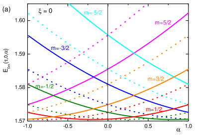
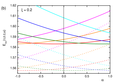
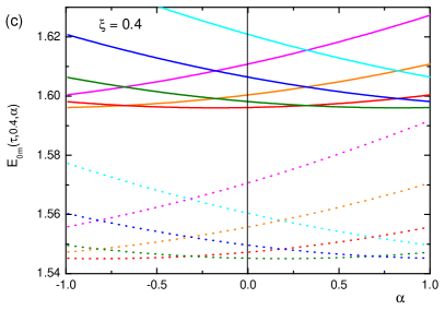
Figure 2: Energy spectrum of positive $E_{0m}(\tau,\xi,\alpha)$. For convenience we choose $v_{F}=w=1$ and $a=10$. The solid and dotted lines correspond to $\tau=1$ and $\tau=-1$, respectively. The colors pink, orange, red, green, blue, and cyan correspond to $m=5/2$, $3/2$, $1/2$, $-1/2$, $-3/2$, and $-5/2$, respectively. (a) is the energy spectrum when $\xi=0$, the case without interaction which is identical to Ref. [9]. (b) and (c) are the energy spectra when the interaction exists. Note that, besides the breaking of valley degeneracy, the spectrum of the $\tau=+1$ valley is raised and the spectrum of the $\tau=-1$ valley is lowered.

In Fig. 2 we plot the first few positive energy levels with $n=0$ as a function of the magnetic flux $\alpha$ for different values of $\xi$. In the figure the solid and dotted lines correspond to $\tau=1$ and $\tau=-1$, respectively. Fig. 2(a) is the plot of $\alpha$-dependence when the Coulomb interaction is zero, which is the same situation as Ref. [9]. For the analysis of the energy spectrum with $\xi=0$, we let $E_{0m}(\tau,0,\alpha)=E(\tau,m,\alpha)$. When $\alpha=0$, since the time reversal symmetry by $\mathcal{T}$ is preserved, there are degeneracies between $E(1,m,0)$ and $E(-1,-m,0)$. However, the intravalley degeneracy is broken, that is, $E(\tau,m,0)\neq E(\tau,-m,0)$ because of the confinement potential that breaks the effective time reversal symmetry by $\bm{\Theta}$. Obviously, when $\alpha\neq 0$, these degeneracies are broken due to the AB potential.

Fig. 2(b) and Fig. 2(c) are the plots of $\alpha$-dependence when $\xi=0.2$ and $\xi=0.4$, the case of repulsive interaction. As noted from the figures, the splitting of the intravalley degeneracy still exists due to the mass terms of the scalar coupling and the confinement potential. What is more interesting here is that the scalar coupling raises the whole energy spectrum of the $\tau=+1$ valley and lowers the whole energy spectrum of the $\tau=-1$ valley. The situation will be reversed if the interaction is attractive; the $\tau=-1$ valley is raised, while the $\tau=+1$ valley is lowered. As explained in Sec. 2 this effect is ascribed to the TRS breaking by the scalar coupling of $\xi/r$ entered as a mass term in the Dirac equation.

Another interesting feature to be noted is that the separation between the two spectra gets larger as the interaction strength increases. To see the energy difference between the two separated spectra, we look into the $\tau$-dependent part in the Eq. (95) for a fixed set of $(n,m,\alpha)$. The energy difference is then determined by the term $\mathcal{E}_{nm}(\tau,\xi,\alpha)$ which can be positive or negative depending on the sign of $\tau$ together with $\eta$ and $\omega_{1}$. With the assumption (88), since $\eta\omega_{1}\sim\vartheta\xi$ ($\vartheta$ a positive constant), we may write $\mathcal{E}_{nm}(\tau,\xi,\alpha)\propto\epsilon(\tau\xi)\xi\sqrt{\eta^{2}+\xi^{2}}$, which becomes positive when $\tau\xi>0$ and negative when $\tau\xi<0$. Thus, for a repulsive interaction for which $\xi>0$, the energy spectrum of $\tau=+1$ valley is raised, while that of $\tau=-1$ valley is lowered; for the attractive interaction, since $\xi<0$, the opposite occurs. The energy difference between the two spectra is then $\Delta\mathcal{E}_{nm}\propto\xi\sqrt{\eta^{2}+\xi^{2}}$, which explains the increase of the separation with $\xi$.

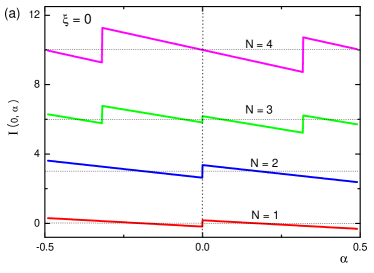
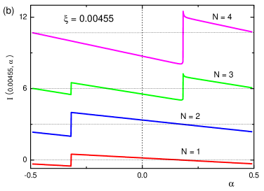
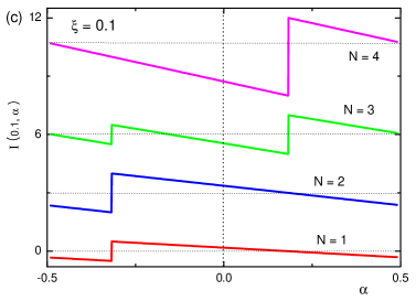
Figure 3: Persistent currents as a function of $\alpha$ for different values of $\xi$. $N$ is the number of electrons in the occupied states. (a) is when $\xi=0$, the case without Coulomb interaction. (b) and (c) are the cases with Coulomb interaction through the scalar coupling. Note that persistent currents are symmetric about $\alpha=0$ when $\xi=0$, but asymmetric about $\alpha=0$ when $\xi>0$. The latter is ascribed to the separation between the spectrum of $\tau=+1$ valley and that of $\tau=-1$ valley.

A possible way of observing the splittings of valley degeneracies is to measure the magnetic moment induced by persistent current in the graphene ring [26]. The persistent current can be obtained from the energy eigenvalues and, at zero temperature, it is given by

$$\displaystyle I(\xi,\alpha)=-\sum_{\tau=\pm 1}\sum_{n}\sum_{m}\frac{\partial}{\partial\alpha}E_{nm}(\tau,\xi,\alpha).$$ (96)

In Fig. 3 we present the persistent current as a function of the magnetic flux $\alpha$ for different values of $\xi$ and the number of electrons $N$ (including spin). Fig. 3(a) is the plot when $\xi=0$, the case without interaction. Since the intervalley degeneracy exists the current is symmetric about $\alpha=0$ when there are equal number of electrons at each valley, as can be seen from the figure. When $\xi>0$ and large, the separation between the two spectra of $\tau=\pm 1$ valleys is large. Since the electrons occupy from the lowest levels at zero temperature the states of the lower spectrum (the $\tau=-1$ valley) will be occupied first, while those of the higher spectrum (the $\tau=+1$ valley) are almost empty. Thus, the persistent current is contributed largely by the lower valley electrons, and becomes essentially a single valley phenomenon, known as valley polarization. This should produce an asymmetric persistent current about $\alpha=0$ and a finite value at $\alpha=0$, which are illustrated in Figs. 3(b) and 3(c). As we can notice in Fig. 3(b), even for very small value of the interaction strength, the qualitative feature is quite different from the case without the interaction because of its role of symmetry breaking. We also emphasize that the $\alpha$-dependences of persistent currents for $\xi>0$ are essentially the same because the electrons occupy only the energy levels in the lower spectrum corresponding to the $\tau=-1$ valley.

4 ABC problem with vector coupling

In this section we consider the vector coupling of the potential $\xi/r$. Here we will use the term Coulomb potential because the vector coupling is related to the electric Coulomb potential. Using the Hamitonian given in Eq. (22) the Dirac equation inside the ring can be written as

$$\displaystyle{\bm{\sigma}}\cdot\left(\bm{p}+e\bm{A}\right)\psi=\left(\tilde{E}-\frac{\tilde{\xi}}{r}\right)\psi$$ (97)

Operating ${\bm{\sigma}}\cdot\left(\bm{p}+e\bm{A}\right)$ on the equation and following the same procedure as in the previous section the reduced radial equation is given by

$$\eqalign{\left[\partial_{r}^{2}+\frac{1}{r}\partial_{r}-\frac{\eta^{2}+1/4}{r^{2}}+\left(\tilde{E}^{2}-\frac{\tilde{\xi}}{r}\right)^{2}\right]\left(\begin{array}[]{c}f_{1m}(r)\\ f_{2m}(r)\end{array}\right)\cr=-\frac{1}{r^{2}}\epsilon(\eta)\sqrt{\eta^{2}-{\tilde{\xi}}^{2}}\sigma_{3}\left(\begin{array}[]{c}f_{1m}(r)\\ f_{2m}(r)\end{array}\right).}$$ (104)

Here, the two components $(f_{1m}(r),f_{2m}(r))$ are related to the spinor $\chi(r)$ as follows:

$$\chi(r)=\left(\begin{array}[]{c}\chi_{1m}(r)\\ \chi_{2m}(r)\end{array}\right)=U_{v}^{-1}\left(\begin{array}[]{c}f_{1m}(r)\\ f_{2m}(r)\end{array}\right),$$ (105)

where the transformation matrix $U_{v}$ is defined by

$$\eqalign{U_{v}^{\pm 1}=\cosh\frac{\phi}{2}\,\sigma_{0}\pm\epsilon(\tilde{\xi})\epsilon(\eta)\,\sinh\frac{\phi}{2}\,\sigma_{2}\cr\tanh\frac{\phi}{2}=\epsilon(\tilde{\xi})\frac{|\eta|-\sqrt{\eta^{2}-{\tilde{\xi}}^{2}}}{\tilde{\xi}}}$$ (108)

and satisfies the matrix diagonalization $\eta\sigma_{3}-i\tilde{\xi}\sigma_{1}=\epsilon(\eta)\sqrt{\eta^{2}-\tilde{\xi^{2}}}U_{v}^{-1}\sigma_{3}U_{v}$. Note that $U_{v}$ in Eq. (105) is not unitary.

The solutions of Eq. (104) are expressed in terms of the confluent hypergeometric functions:

$$\eqalign{f_{1m}(\rho)=e^{i\rho}(-2i\rho)^{t_{-}}\left[C_{1m}M(a_{-},\,b_{-},\,-2i\rho)+D_{1m}U(a_{-},\,b_{-},\,-2i\rho)\right]\cr f_{2m}(\rho)=e^{i\rho}(-2i\rho)^{t_{+}}\left[C_{2m}M(a_{+},\,b_{+},\,-2i\rho)+D_{2m}U(a_{+},\,b_{+},\,-2i\rho)\right]}$$ (111)

where $M(a,b,\rho)$ and $U(a,b,\rho)$ are the Kummer’s functions [27], $\rho=|\tilde{E}|r$, and $a_{\pm}$, $b_{\pm}$ and $t_{\pm}$ are given by

$$a_{\pm} = t_{\pm}+\frac{1}{2}+i\epsilon(\tilde{E})\tilde{\xi},\quad b_{\pm}=2t_{\pm}+1$$

$$t_{\pm} = \sqrt{\eta^{2}-{\tilde{\xi}}^{2}}\pm\frac{\epsilon(\eta)}{2}.$$ (112)

By the same method as in Sec. II and exploiting the recurrence relations and differential properties of the confluent hypergeometric functions, one can derive the following relations between coefficients after some algebra;

$$C_{2m}=\epsilon(E)c_{21}C_{1m}\qquad D_{2m}=\epsilon(E)d_{21}D_{1m},$$ (113)

where

$$c_{21}=-\left(\frac{|\eta|}{4(\eta^{2}-\tilde{\xi}^{2})+2\sqrt{\eta^{2}-\tilde{\xi}^{2}}}\right)^{\epsilon(\eta)},\qquad d_{21}=\left(\frac{\sqrt{\eta^{2}-\tilde{\xi}^{2}}+i\epsilon(E)\tilde{\xi}}{|\eta|}\right)^{\epsilon(\eta)}.$$ (114)

Substituting the solutions (111) with the relation (113) into the transformation equation (105) we can write the eigenspinor $\chi(\rho)$ as

$$\left(\begin{array}[]{c}\chi_{1m}(\rho)\\ \chi_{2m}(\rho)\end{array}\right)=e^{i\rho}(-2i\rho)^{t_{-}}\left(\begin{array}[]{cc}m_{1}(\rho)&u_{1}(\rho)\\ m_{2}(\rho)&u_{2}(\rho)\end{array}\right)\left(\begin{array}[]{c}C_{1m}\\ D_{1m}\end{array}\right)$$ (121)

where

$$\eqalign{m_{1}(\rho)=\cosh\frac{\phi}{2}\,M(a_{-},b_{-},-2i\rho)+i\epsilon(\tilde{\xi}\eta E)(-2i\rho)^{\epsilon(\eta)}\,c_{21}\sinh\frac{\phi}{2}M(a_{+},b_{+},-2i\rho)\cr u_{1}(\rho)=\cosh\frac{\phi}{2}\,U(a_{-},b_{-},-2i\rho)+i\epsilon(\tilde{\xi}\eta E)(-2i\rho)^{\epsilon(\eta)}\,d_{21}\sinh\frac{\phi}{2}U(a_{+},b_{+},-2i\rho)\cr m_{2}(\rho)=\epsilon(E)(-2i\rho)^{\epsilon(\eta)}\,c_{21}\cosh\frac{\phi}{2}\,M(a_{+},b_{+},-2i\rho)-i\epsilon(\tilde{\xi}\eta)\sinh\frac{\phi}{2}M(a_{-},b_{-},-2i\rho)\cr u_{2}(\rho)=\epsilon(E)(-2i\rho)^{\epsilon(\eta)}\,d_{21}\cosh\frac{\phi}{2}\,U(a_{+},b_{+},-2i\rho)-i\epsilon(\tilde{\xi}\eta)\sinh\frac{\phi}{2}U(a_{-},b_{-},-2i\rho).}$$ (126)

To proceed we use the same infinite mass boundary condition introduced in Sec. II. Inserting Eq. (121) into the boundary condition (78) it is straightforward to show

$$\eqalign{\left[m_{2}(\rho_{2})-i\tau m_{1}(\rho_{2})\right]C_{1m}+\left[u_{2}(\rho_{2})-i\tau u_{1}(\rho_{2})\right]D_{1m}=0\cr\left[m_{2}(\rho_{1})+i\tau m_{1}(\rho_{1})\right]C_{1m}+\left[u_{2}(\rho_{1})+i\tau u_{1}(\rho_{1})\right]D_{1m}=0,}$$ (129)

where $\rho_{1}=|\tilde{E}|(a-w/2)$ and $\rho_{2}=|\tilde{E}|(a+w/2)$. The secular equation requires then the following condition:

$$\frac{m_{2}(\rho_{2})-i\tau m_{1}(\rho_{2})}{m_{2}(\rho_{1})+i\tau m_{1}(\rho_{1})}=\frac{u_{2}(\rho_{2})-i\tau u_{1}(\rho_{2})}{u_{2}(\rho_{1})+i\tau u_{1}(\rho_{1})}.$$ (130)

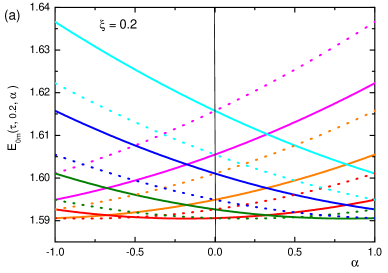
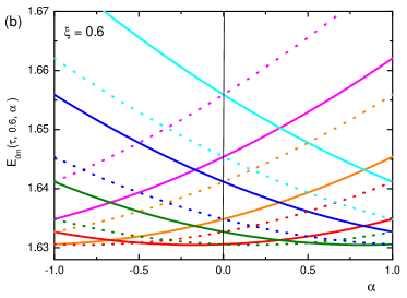
Figure 4: Energy spectrum for the vector coupling. For convenience we choose $v_{F}=w=1$ and $a=10$. The solid and dotted lines correspond to $\tau=1$ and $\tau=-1$, respectively. The colors pink, orange, red, green, blue, and cyan correspond to $m=5/2$, $3/2$, $1/2$, $-1/2$, $-3/2$, and $-5/2$, respectively. (a) and (b) are energy spectra for $\xi=0.2$ and $\xi=0.6$, respectively. Note that the intervalley symmetry about $\alpha=0$ is still kept here even in the presence of the potential and the whole spectrum is raised by $\xi/a$ compared to the Fig. 2(a).

To obtain the eigenvalue spectrum we impose the same condition with Eq. (88) and use the asymptotic formula of the confluent hypergeometric functions for large $\rho$. Expanding Eq. (130) up to the second order of perturbation, one can show that the energy eigenvalue satisfies

$$|E|=\frac{v_{F}}{w}\left[\left(n+\frac{1}{2}\right)\pi+2\epsilon(E)\tilde{\xi}\left(\frac{w}{2a}\right)+\eta^{2}\left(\frac{v_{F}}{|E|a}\right)\left(\frac{w}{2a}\right)-\frac{\tau}{2}\epsilon(E)\eta\left(\frac{v_{F}}{|E|a}\right)^{2}\right],$$ (131)

where $n$ is a non-negative integer. Solving Eq. (131) by iteration and keeping only leading terms, we obtain the energy eigenvalues

$$E_{nm}(\tau,\xi,\alpha)=\pm\varepsilon_{n}\pm\lambda_{n}\eta\left(\eta\mp\frac{\tau}{\left(n+\frac{1}{2}\right)\pi}\right)+\frac{\xi}{a},$$ (132)

where $\varepsilon_{n}=v_{F}(n+1/2)/w$ $(n=0,1,2,\dots)$ and $\lambda_{n}=(v_{F}/a)^{2}/2\varepsilon_{n}$, and the $\alpha$ dependence is through the variable $\eta$ defined in Eq. (49).

We can immediately see from Eq. (132) that the effect of the potential $\xi/r$ in the vector coupling is merely an additive constant $(\xi/a)$, shifting the whole spectrum of energy eigenvalues. It also reveals the complete decoupling between the AB and the Coulomb effects, because the Coulomb effect appears in the first order whereas the AB effect arises in the second order perturbation. In Fig. 4, we show the energy spectrum in which the symmetry between the two valley spectra about $\alpha=0$ is manifested, representing the existence of the intervalley degeneracy. As discussed in Sec. 2, the Hamiltonian without AB potential in Eq. (97) is invariant under the time reversal operators $\mathcal{T}$ and $\bm{\Theta}$, and hence the vector coupling breaks neither the intervalley nor the intravalley degeneracies. It is thus expected that the eigenvalue spectrum in the vector coupling has essentially the same feature as the spectrum without the Coulomb interaction. By the same reason, the Coulomb potential in the vector coupling does not alter the behavior of the persistent current and hence it is symmetric about $\alpha=0$ as shown in Fig. 3(a).

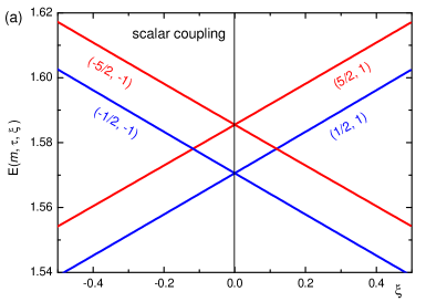
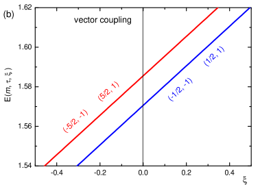
Figure 5: The $\xi$-dependence of the energy spectrum when there is no AB potential (that is, when $\alpha=0$). For convenience we let $E_{0m}(\tau,\xi,0)=E(m,\tau,\xi)$, and the parenthesis denotes $(m,\tau)$. (a) and (b) correspond to the scalar coupling and the vector coupling for $m=\pm 1/2,\pm 5/2$ and $\tau=\pm 1$, respectively. The splitting of intervalley degeneracy is clearly seen in (a), but it is not broken in (b).

In Fig. 5, we also present the energy spectrum as a function of $\xi$ without the AB potential to compare the bare effects of the Coulomb type potential between the scalar coupling and the vector coupling. Fig. 5(a) shows the splitting of intervalley degeneracy due to the symmetry-breaking term in the scalar coupling. However, in Fig. 5(b), we see that no intervalley splitting exists in the case of vector coupling. This also confirms that, in the case of vector coupling, the Coulomb potential alone does not break the intervalley degeneracy, as explained by the consideration of the time reversal symmetry.

5 Conclusion

In this paper we have considered the ABC problem in a graphene ring with magnetic flux tube and a Coulomb type potential $\xi/r$ at its center. We have investigated the effects of the potential on the energy spectrum in two different ways: the scalar coupling and the vector coupling. In the scalar coupling the potential enters the 2D Dirac equation as a symmetry-breaking mass term, so that both the intervalley and the intravalley degeneracies are broken. The main effect of the interaction appears as the separation between the energy spectrum of one valley and that of the other valley, which is attributed to the breaking of the intervalley degeneracy; for the repulsive interaction the $\tau=+1$ ($\bm{K}$) valley is lifted while the $\tau=-1$ ($\bm{K^{\prime}}$) valley is lowered, and vice versa for the attractive interaction. Contrary to the scalar coupling, the potential in the vector coupling does not break any symmetry and only shifts the AB energy spectrum, indicating essentially the same feature as the energy spectrum without a Coulomb potential.

The results obtained here suggests that the scalar coupling of the Coulomb type potential $\xi/r$ can decouple the two valleys because of the considerable lift of energy spectrum, so that each valley degree of freedom becomes an independent quantity, called a valley isospin. A real experiment with graphene ring may realize this decoupling, known as the valley polarization, which is an important element in the graphene-based electronics, called valleytronics [18, 28].

Another interesting issue related to the AB effect is when the thin magnetic flux tube is located at the center of the honeycomb lattice shown in Fig. 1(a). Since the anyon is a flux-carrying particle, a similar situation arises when there is an anyon impurity in the graphene plane. Since, in this case, the magnetic flux is located on the graphene, we should treat the singular solution problem, which was extensively discussed in Refs. [29, 30] in the context of the anyonic and cosmic string theories. Roughly speaking, there are two prescriptions for the interpretation of the singular solution: one is a mathematically-based prescription called self-adjoint extension and the other is a physically-based prescription. We do not know yet which prescription is physically more reasonable. Probably, the real experiment with graphene may shed light on the treatment of the singular solution. If so, our understanding on the anyonic and cosmic string theories can be greatly enhanced through the graphene physics. We will explore this issue in the future.

References

References

• [1] Wallace P R 1947 Phys. Rev.71 622
• [2] For a recent review of graphene, see Castro Neto A H, Guinea F, Peres N M R, Novoselov K S and Geim A K 2009 Rev. Mod. Phys.81 109
• [3] Slonczewski J C and Weiss P R 1958 Phys. Rev.109 272
• [4] Semenoff G W 1984 Phys. Rev. Lett.53 2449;
DiVincenzo D P and Mele E J 1984 Phys. Rev.B 29 1685
• [5] Haldane F D M 1988 Phys. Rev. Lett.61 2015
• [6] Jackiw R 1990 Nucl. Phys.B(Proc. Suppl.) 18 107
• [7] Jackiw R and Pi S Y 2007 Phys. Rev. Lett.98 266402;
Pachos J K and Stone M 2007 Int. J. Mod. Phys. B 21 5113;
Allor D, Cohen T D, and McGady D A 2008 Phys. Rev.D 78 096009;
Beneventano C G and Santangelo E M 2008 J. Phys. A: Math. Gen.41 (2008) 164035; Jackiw R and Pi S Y 2008 Phys. Rev.78 (2008) 132104;
Beneventano C G, Giacconi P, Santangelo E M, and Soldati R 2009 J. Phys. A: Math. Gen.42 275401;
Bordag M, Fialkovsky I V, Gitman D M, and Vassilevich D V 2009 Phys. Rev.B 80 245406;
Semenoff G W 2011 Phys. Rev.B 83 115450;
Iorio A 2011 Ann. Phys. 326 1334;
Drissi L B, Saidi E H, and Bousmina M 2010 Nucl. Phys.B 829 523
• [8] Aharonov Y and Bohm D 1959 Phys. Rev.115 485
• [9] Recher P, Trauzettel B, Rycerz A, Blater Y M, Beenakker C W J and Morpurgo A F 2007 Phys. Rev.B 76 235404
• [10] Rycerz A 2009 Acta. Phys. Pol. A 115 322;
Wurm J, Wimmer M, Baranger H U, and Richter K 2010 Semicond. Sci. Technol. 25 034003
• [11] Jackiw R, Milstein A I, Pi S Y and Terekhov I S 2009 Phys. Rev.B 80 033413; Katsnelson M I 2010 Europhys. Lett. 89 17001;
Schelter J, Bohr D and Trauzettel B 2010 Phys. Rev.B 81 195441
• [12] Russo S et al 2008 Phys. Rev.B 77 085413;
Molitor F et al 2010 New J. Phys.12 043054
• [13] Kibler M and Negadi T 1987 Phys. Lett.A 124 42;
Doebner H D and Papp E 1990 Phys. Lett.A 144 423
• [14] Villalba V M 1995 J. Math. Phys.36 3332
• [15] Lévy-Leblond J M 1967 Commun. Math. Phys. 6 286
• [16] Hagen C R and Park D K 1996 Ann. Phys. 251 45
• [17] Akmerov A R and Beenakker C W J 2007 Phys. Rev. Lett.98 157003;
• [18] Rycerz A, Tworzydlo J and Beenakker C W J 2007 Nat. Phys. 3 172;
Trauzettel B, Bulaev D V, Loss D and Burkard G 2007 Nat. Phys. 3 192;
Recher P, Nilsson J, Burkard G and Trauzettel B 2009 Phys. Rev.B 79 085407
• [19] Suzuura H and Ando T 2002 Phys. Rev. Lett.89 266603
• [20] Beenakker C W J 2008 Rev. Mod. Phys.80 1337
• [21] Berry M V and Mondragon R J 1987 Proc. R. Soc. London A 412 53
• [22] McCann Edward and Fal’ko Vladimir I. 2004 J. Phys. C: Solid State Phys.16 2371
• [23] Capri Anton Z  1977 Am. J. Phys. 45 823
• [24] Bonneau G, Faraut J and Valent G 2001 Am. J. Phys. 69 322
• [25] Dombey N and Calogeracos A 1999 Phys. Rep. 315 41
• [26] Lévy L P, Dolan G, Dunsmuir J and Bouchiat H 1990 Phys. Rev. Lett.64 2074;
Chandrasekhar V, Webb R A, Ketchen M B, Gallagher W J, Brady J J and Kleinsasser A 1991 Phys. Rev. Lett.67 3578;
Bleszynski-Jayich A C, Shanks W E, Peaudecerf B, Ginossar E, von Oppen F, Glazman L, and Harris J G E 2009 Science 326 272
• [27] 1970 Hanbook of Mathematical Functions ed M Abramowitz and I A Stegun (New York: Dover) p.504
• [28] Zhou S Y, Gweon G -H, Fedorov A V, First P N, De Heer W A, Lee D -H, Guinea F, Castro Neto A H and Lanzara A 2007 Nat. Mater. 6 770
• [29] Jackiw R 1991 Delta function potential in two- and three-dimensional quantum mechanics M A B Beg memorial volume ed A Ali and P Hoodbhoy (Singapore: World Scientific);
de Sousa Gerbert Ph 1989 Phys. Rev.40 1346;
Hagen C R 1990 Phys. Rev. Lett. 64 503;
Park D K 1995 J. Math. Phys. 36 5453
• [30] Alford M G and Wilczek F 1989 Phys. Rev. Lett.62 1071;
Alford M G, March-Russell J and Wilczek F 1989 Nucl. Phys.B 328 140;
Chen Y H, Wilczek F, Witten E and Halperin B I 1989 Int. J. Mod. Phys. B 3 1001