Global asymptotic properties for a Leslie-Gower food chain model

Abstract

We study global asymptotic properties of a continuous time Leslie-Gower food chain model. We construct a Lyapunov function which enables us to establish global asymptotic stability of the unique coexisting equilibrium state.

In his papers Les_48 ; Les._58 , P.H. Leslie introduced a predator-prey model where both interacting species are assumed to grow according to the logistic law. That is both species grow with a rate that is initially (for small population) proportional to the population and is limited by a carrying capacity. The novel feature of this model is that, while the carrying capacity for the prey is a positive constant, the carrying capacity of the predator’s environment is proportional to the prey population. This idea leads to a model that is quite different from the Lotka-Volterra predator-prey model. Leslie’s model stresses the fact that there are upper limits to the rates of increase of both prey, $H$, and predator, $P$, which are not recognised in the Lotka-Volterra model. These upper limits can be approached under favourable conditions: for the predator, when the number of prey per predator is large; for the prey, when the number of predators (and perhaps the number of prey also) is small. Furthermore, the Leslie-Gower model does not posses the “screw symmetry” that is inherent in the Lotka-Volterra model. This model was initially studied by Leslie and Gower Leslie and Gower , and then by Pielow Pielow . In the case of continuous time, these considerations lead to the differential equations (Pielow, , p. 91)

$$\frac{dH}{dt}=(r-bH-aP)H,\qquad\frac{dP}{dt}=\left(q-c\frac{P}{H}\right)P.$$ (1)

Here $H(t)$ and $P(t)$ are the prey and the predator populations respectively; $r$ and $q$ are the growth rates of the prey and the predator respectively; $a$ is the attack rate; $1/rb$ is the carrying capacity of the prey environment, and $1/qc$ is the efficiency of consumption for the predator (that is $H(t)/qc$ is the predator population that the prey population of the size $H$ can support). All the constants in the system (1) are positive. This model always has the unique coexisting fixed point $Q^{*}=(H^{*},P^{*})$, where

$$H^{*}=\frac{rc}{aq+bc},\qquad P^{*}=\frac{rq}{aq+bc},$$ (2)

which was proved to be globally asymptotically stable Korobeinikov_2001 .

The Leslie-Gower model can be immediately extended to the case of a food chain. The food chain composed of $n+1$ levels where the $i$th level depends (predates) upon only the $i-1$ level can be represented by the transfer diagram

$$H\longrightarrow P_{1}\longrightarrow P_{2}\longrightarrow\ldots\longrightarrow P_{n}.$$

This food chain can be described by the following system of differential equations:

$$\frac{dH}{dt} = (r-bH-aP_{1})H,$$

$$\frac{dP_{1}}{dt} = \left(q_{1}-c_{1}\frac{P_{1}}{H}-s_{1}P_{2}\right)P_{1},$$

$$\vdots$$

$$\frac{dP_{i}}{dt} = \left(q_{i}-c_{i}\frac{P_{i}}{P_{i-1}}-s_{i}P_{i+1}\right)P_{i},$$

$$\vdots$$

$$\frac{dP_{n}}{dt} = \left(q_{n}-c_{n}\frac{P_{n}}{P_{n-1}}\right)P_{n}.$$

Here the parameters $q_{i}$, $c_{i}$ and $s_{i}$ are defined by analogy to the single predator case, namely $q_{i}$ is the reproduction rate of the $i$th predator, $c_{i}$ is defined so that $1/q_{i}c_{i}$ is the efficiency of consumption for the $i$th predator, and $s_{i}$ is the attack rate by the $i$th predator. In order for the equations to be biologically meaningful these parameters must all be positive quantities.

The global properties of this model are given by the following Theorem:

Theorem 1.

The Leslie-Gower chain model (Global asymptotic properties for a Leslie-Gower food chain model) always has a positive (coexisting) equilibrium state $Q^{*}_{n}=(H^{*},P^{*}_{1},\ldots,P^{*}_{n})$; this equilibrium state is unique and globally asymptotically stable.

Proof.

(1). Existence of the positive equilibrium state. We prove this by induction. The positive equilibrium state always exists for $n=1$: the coordinates of the equilibrium state are given by equalities (2). We assume that the statement of Theorem holds when $n=m$ and prove that it holds for $n=m+1$ as well.

Starting from an $m$ level chain in which, by assumption, all equilibrium populations $H^{(m)*}$, $P_{i}^{(m)*}$, $i=1,\ldots,m$ are positive, we convert the system to an $m+1$ level chain by introducing a population of top level ($m+1$) predators and allow the system to equilibrate. It can readily be seen that the positive region $\mathbb{R}^{m+1}_{+}$ is an invariant set of this system. That prevents the sign of $P_{i}$ for all $i=1,\ldots,m$ changing. Thus, from the assumption of a positive equilibrium in the $m$ level system, it follows that in the $m+1$ level system all $P_{i}^{(m+1)*}$ for $i=1,\ldots,m$ are positive or zero. Consider the final differential equation

$$\dfrac{\mathrm{d}P_{m+1}}{\mathrm{d}t}=(a-\dfrac{bP_{m+1}}{P_{m}})P_{m+1}.$$ (4)

In order for equilibrium population at $P^{*}_{m+1}=0$ (rather than $P^{*}_{m+1}>0$) to be attained we must have

$$\lim_{P^{*}_{m+1}\rightarrow 0}a-\dfrac{bP^{*}_{m+1}}{P^{*}_{m}}\leq 0.$$ (5)

This requires $\lim_{P^{*}_{m+1}\rightarrow 0}P^{*}_{m}\leq 0$, whereas by assumption that the $m$-level system has a positive equilibrium state the converse holds. Thus the existence of an $m$ level positive equilibrium state implies the existence of an $m+1$ level positive equilibrium state. This completes this section of the proof.

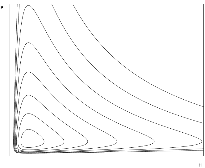
Figure 1: Level curves of the Lyapunov function $\ln\frac{H}{H^{*}}+\frac{H^{*}}{H}+B\left(\ln\frac{P}{P^{*}}+\frac{P^{*}}{P}\right)$.

(2). Global asymptotic stability of the positive equilibrium state. A Lyapunov function

$$V(H,P_{1},\ldots,P_{n})=\left(\ln\frac{H}{H^{*}}+\frac{H^{*}}{H}\right)+\sum_{i=1}^{n}B_{i}\left(\ln\frac{P_{i}}{P_{i}^{*}}+\frac{P_{i}^{*}}{P_{i}}\right),$$

where $B_{i}c_{i}=B_{i-1}s_{i-1}P_{i-1}^{*}$ and $B_{1}c_{1}=aH^{*}$, is defined and continuous for all $H,P_{1},\ldots,P_{n}>0$. The function $V(H,P_{1},\ldots,P_{n})$ satisfies

$$\frac{\partial V}{\partial H}=\frac{1}{H}\left(1-\frac{H^{*}}{H}\right),\qquad\frac{\partial V}{\partial P_{i}}=\frac{B_{i}}{P_{i}}\left(1-\frac{P_{i}^{*}}{P_{i}}\right),$$

and hence the fixed point $Q^{*}_{n}$ is the only extremum of this function. It is easy to see that the point $Q^{*}_{n}$ is the global minimum of $V(H,P_{1},\ldots,P_{n})$ in $\mathbb{R}^{n+1}_{+}$. (Fig. 1 shows the level curves of this function for $n=$1.)

The function $V(H,P_{1},\ldots,P_{n})$ satisfies

$$\frac{dV}{dt} = r-bH-aP_{1}-r\frac{H^{*}}{H}+bH^{*}+a\frac{H^{*}P_{1}}{H}$$

$$+B_{1}\left(q_{1}-c_{1}\frac{P_{1}}{H}-s_{1}P_{2}-q_{1}\frac{P_{1}^{*}}{P_{1}}+c_{1}\frac{P_{1}^{*}}{H}+s_{1}\frac{P_{1}^{*}P_{2}}{P_{1}}\right)$$

$$+\sum_{i=2}^{n-1}B_{i}\left(q_{i}-c_{i}\frac{P_{i}}{P_{i-1}}-s_{i}P_{i+1}-q_{i}\frac{P_{i}^{*}}{P_{i}}+c_{i}\frac{P_{i}^{*}}{P_{i-1}}+s_{i}\frac{P_{i}^{*}P_{i+1}}{P_{i}}\right)$$

$$+B_{n}\left(q_{n}-c_{n}\frac{P_{n}}{P_{n-1}}-q_{n}\frac{P_{n}^{*}}{P_{n}}+c_{n}\frac{P_{n}^{*}}{P_{n-1}}\right)$$

$$= r+\sum_{i=1}^{n}B_{i}q_{i}+bH^{*}-bH-r\frac{H^{*}}{H}+B_{1}c_{1}\frac{P_{1}^{*}}{H}$$

$$-aP_{1}-\sum_{i=2}^{n}B_{i-1}s_{i-1}P_{i}-\sum_{i=1}^{n}B_{i}q_{i}\frac{P_{i}^{*}}{P_{i}}+\sum_{i=2}^{n}B_{i}c_{i}\frac{P_{i}^{*}}{P_{i-1}}$$

$$+a\frac{H^{*}P_{1}}{H}-B_{1}c_{1}\frac{P_{1}}{H}+\sum_{i=1}^{n-1}B_{i}s_{i}\frac{P_{i}^{*}P_{i+1}}{P_{i}}-\sum_{i=2}^{n}B_{i}c_{i}\frac{P_{i}}{P_{i-1}}.$$

By the definition of $B_{i}$, the equalities

$$a\frac{H^{*}P_{1}}{H}-B_{1}c_{1}\frac{P_{1}}{H}=0,\qquad\sum_{i=1}^{n-1}B_{i}s_{i}\frac{P_{i}^{*}P_{i+1}}{P_{i}}-\sum_{i=2}^{n}B_{i}c_{i}\frac{P_{i}}{P_{i-1}}=0$$

hold. Furthermore, recollecting that

$$r=bH^{*}+aP_{1}^{*},\quad q_{i}=c_{i}\frac{P_{i}^{*}}{P_{i-1}^{*}}+s_{i}P_{i+1}^{*},\quad q_{n}=c_{n}\frac{P_{n}^{*}}{P_{n-1}^{*}}$$

hold at $Q^{*}_{n}$, we obtain

$$\sum_{i=1}^{n}B_{i}q_{i}=B_{1}c_{1}\frac{P_{1}^{*}}{H^{*}}+\sum_{i=2}^{n}B_{i}c_{i}\frac{P_{i}^{*}}{P_{i-1}^{*}}+\sum_{i=1}^{n}B_{i}s_{i}P_{i+1}^{*}=aP_{1}^{*}+2\sum_{i=2}^{n}B_{i-1}s_{i-1}{P_{i}^{*}},$$

$$r\frac{H^{*}}{H}-B_{1}c_{1}\frac{P_{1}^{*}}{H}=bH^{*}\frac{H^{*}}{H},$$

and

$$\sum_{i=1}^{n}B_{i}q_{i}\frac{P_{i}^{*}}{P_{i}}-\sum_{i=2}^{n}B_{i}c_{i}\frac{P_{i}^{*}}{P_{i-1}} = B_{n}q_{n}\frac{P_{n}^{*}}{P_{n}}+\sum_{i=1}^{n-1}B_{i}\left(q_{i}-s_{i}P_{i+1}^{*}\right)\frac{P_{i}^{*}}{P_{i}}$$

$$= aP_{1}^{*}\frac{P_{1}^{*}}{P_{1}}+\sum_{i=2}^{n}B_{i}c_{i}\frac{P_{i}^{*}}{P_{i-1}^{*}}\frac{P_{i}^{*}}{P_{i}}$$

$$= aP_{1}^{*}\frac{P_{1}^{*}}{P_{1}}+\sum_{i=2}^{n}B_{i-1}s_{i-1}P_{i}^{*}\frac{P_{i}^{*}}{P_{i}}.$$

Therefore,

$$\frac{dV}{dt} = bH^{*}\left(2-\frac{H^{*}}{H}-\frac{H}{H^{*}}\right)$$

$$+aP_{1}^{*}\left(2-\frac{P_{1}^{*}}{P_{1}}-\frac{P_{1}}{P_{1}^{*}}\right)+\sum_{i=2}^{n}B_{i-1}s_{i-1}P_{i}^{*}\left(2-\frac{P_{i}^{*}}{P_{i}}-\frac{P_{i}}{P_{i}^{*}}\right)$$

$$= -bH\left(1-\frac{H^{*}}{H}\right)^{2}+aP_{1}\left(1-\frac{P_{1}^{*}}{P_{1}}\right)^{2}+\sum_{i=2}^{n}B_{i-1}s_{i-1}P_{i}\left(1-\frac{P_{i}^{*}}{P_{i}}\right)^{2}.$$

That is, for this model $\frac{dV}{dt}<0$ strictly holds for all $H,P_{1},\ldots,P_{n}>0$, except the fixed point $Q^{*}_{n}$ where $\frac{dV}{dt}=0$. Therefore, by the Lyapunov asymptotic stability theorem Lyapunov , the fixed point $Q^{*}$ is globally asymptotically stable.

(3). Uniqueness of the positive equilibrium state. At any equilibrium state, $\frac{dV}{dt}=0$ must hold. For this model, however, the fixed point $Q^{*}_{n}$ is the only point in $\mathbb{R}_{+}^{n+1}$ where $\frac{dV}{dt}=0$ holds.

This completes the proof. ∎

Apart from the positive equilibrium state $Q^{*}_{n}$ where all $n+1$ species coexist, this system also has $n$ equilibrium states $Q^{*}_{k}$ (where $k=0,1,\ldots,n-1$), which corresponds to the reduced $m$-species food chains

$$H\longrightarrow P_{1}\longrightarrow P_{2}\longrightarrow\ldots\longrightarrow P_{k}.$$

Biologically these correspond to the case in which some external intervention has reduced the population of the $i$th species to zero (we have proved above that this system is uniformly persistent, and hence that can never occur for this model via the natural evolution of the system) leading to the extinction of the $i+1$th level species that feeds on species $i$, and then to all higher levels of the food chain. For each of these equilibrium states, $H,P_{1},\ldots,P_{k}>0$ while $P_{k+1}=\ldots=P_{n}=0$. Thus, $Q^{*}_{0}$ corresponds to the predator-free case and has the coordinates $H_{0}=r/b,P_{1}=\ldots=P_{n}=0$; $Q^{*}_{1}$ coincides with the equilibrium state (2) of the two-species model (1). The following Corollary immediately follows from the Theorem:

Corollary 1.

Apart from the positive equilibrium state $Q^{*}_{n}$, the system has $n$ non-negative equilibrium states $Q^{*}_{k}$ (where $k=0,1,\ldots,n-1$). Each of these equilibrium states is unstable in $\mathbb{R}^{n}_{\geq 0}$, but globally asymptotically stable in the $k$-dimensional invariant subspace $\mathbb{R}^{k}_{+}=\{H,P_{1},\ldots,P_{k}>0;P_{k+1}=\ldots=P_{n}=0\}$.

In conclusion, we have to note that, apart from the mentioned $n+1$ equilibrium states that are located in the nonnegative region $\mathbb{R}^{n}_{\geq 0}$, the system has other $n-1$ points with the coordinates that satisfy the equalities

$$r=bH+aP_{1},\quad q_{i}=c_{i}\frac{P_{i}}{P_{i-1}}+s_{i}P_{i+1},\quad q_{n}=c_{n}\frac{P_{n}}{P_{n-1}}.$$

Indeed, it is readily seen that this system of algebraic equations is equivalent to a polynomial of the degree $n$ and that this system has no complex solutions. However, the existence of these equilibria do not contradict the Theorem since these points are located outside of the non-negative region $\mathbb{R}^{n}_{\geq 0}$, which is the phase space of the system. The origin is an unstable equilibrium state of the system as well.

These results demonstrate both the practicality and the usefulness of performing a stability analysis on non-trivial ecosystem models. We have shown, using a Leslie-Gower food chain model as an example, that it is possible to enumerate and characterize the stability properties of all the equilibrium states of the model.

References

• (1) (1836072) A. Korobeinikov, A Lyapunov function for Leslie-Gower predator-prey models, Appl. Math. Letters, 14 (2001), 697–699.
• (2) (0027991) P. H. Leslie, Some further notes on the use of matrices in population mathematics, Biometrika, 35 (1948), 213–245.
• (3) (0093436) P. H. Leslie, A stochastic model for studying the properties of certain biological systems by numerical methods, Biometrika, 45 (1958), 16–31.
• (4) (0122603) P. H. Leslie and J. C. Gower, The properties of a stochastic model for the predator-prey type of interaction between two species, Biometrica, 47 (1960), 219–234.
• (5) (1229075) A. M. Lyapunov, “The General Problem of the Stability of Motion,” Taylor & Francis, London, 1992.
• (6) (0434494) E. C. Pielou, “Mathematical Ecology,” John Wiley & Sons, New York, 1977.