Quantum $A_{r}$ $Q$-system solutions as q-multinomial series

Abstract.

We derive explicit expressions for the generating series of the fundamental solutions of the $A_{r}$ quantum $Q$-system of Ref. [P. Di Francesco and R. Kedem, Noncommutative integrability, paths and quasi-determinants, preprint arXiv:1006.4774 [math-ph]], expressed in terms of any admissible initial data. These involve products of quantum multinomial coefficients, coded by the initial data structure.

1. Introduction

The study of some discrete integrable systems, taking the form of recursion relations, i.e. evolution equations in a discrete time $n\in{\mathbb{Z}}$ with suitable conservation laws, has recently shed some new light [3] on the positivity conjecture of cluster algebras [8]. Indeed, admissible sets of initial data for such systems are particular clusters in some specific, non-finite type cluster algebras, whereas cluster mutations are implemented by the update of initial data via local application of the evolution equation. The positivity conjecture for cluster algebras then boils down to the following property: the solutions of such systems are Laurent polynomials with non-negative integer coefficients of any of their admissible initial data.

In [3], this was proved for the so-called $Q$-system for $A_{r}$, by expressing solutions as partition functions for weighted paths on some target graphs, the weights being explicit Laurent monomials of initial data. An extremely useful tool for such representations is the notion of (multiply branching) continued fraction. We were able to prove that mutations of initial data are implemented by local rearrangement of the continued fraction expressions for the generating series of fundamental solutions of the $Q$-system. This was then extended to the so-called $T$-systems in [5] for initial data forming periodic stepped surfaces, and finally to the most general initial data in [2], by use of a manifestly positive network path formulation. In all these cases, positivity follows from a form of discrete path integral representation of the solutions.

The cluster algebra structure has a natural quantum version [1], in which cluster variables obey quantum commutation relations within each cluster. This led to the natural definition of quantum $Q$-systems [7]. In an analogous spirit, it was shown in [5] that the $T$-system may be viewed as a $Q$-system, involving non-commutative (time-ordered) variables. An even broader non-commutative version is known for the fully non-commutative $A_{1}$ $Q$-system, for which Laurent positivity was conjectured by M. Kontsevich, and subsequently proved in [6]. The latter proof relies on an extension of the previous path formulations to paths with non-commutative step weights: the partition function of such paths is the sum over paths of the product of step weights taken in the same order as the steps are taken. In [7], such paths were used to investigate non-commutative versions of the $Q$-systems. In particular, a compact formulation in terms of non-commutative continued fractions was obtained.

Except in very specific cases, very few explicit expressions of cluster variables in terms of fundamental data are known. For the (classical) $A_{r}$ $Q$-system, such expressions were derived in [4] for the generating series of its fundamental solutions.

The aim of this note is to generalize these expressions for the generating series of the fundamental solutions of the quantum $A_{r}$ $Q$-system, by using the non-commutative continued fraction expressions of [7]. The results are summarized in our main Theorem 3.12 below, which expresses these generating functions for any admissible initial data as explicit series with coefficients that are Laurent polynomials with coefficients in ${\mathbb{Z}}_{+}[q,q^{-1}]$, where $q$ is the parameter of the quantum deformation.

Acknowledgments: We thank R. Kedem for helpful discussions and the Mathematical Sciences Research Institute, Berkeley, for hospitality during the program “Random Matrix Theory, Interacting Particle Systems and Integrable Systems” (fall 2010) during which this work was initiated.

2. The quantum $A_{r}$ $Q$-system: definitions

2.1. The system

Let $\lambda_{i}=i(r+1-i)$, $i=1,2,...,r$ and $q\in{\mathbb{C}}^{*}$. The $A_{r}$ quantum $Q$-system [7] is an evolution equation for variables $R_{i,j}$, $i\in[1,r]$ and $j\in Z$, elements of a non-commuting unital algebra:

(2.1) $$q^{\lambda_{i}}\,R_{i,j+1}R_{i,j-1}=R_{i,j}^{2}+R_{i+1,j}R_{i-1,j}\qquad(i\in[1,r],j\in{\mathbb{Z}})$$

with $R_{0,j}=R_{r+1,j}=1$ for all $j\in{\mathbb{Z}}$.

2.2. Initial data

This is a three-term recursion relation in the variable $j$, which allows to determine all $R_{i,j}$ in terms of any initial data covering two consecutive values of $j$. Initial data are indexed by Motzkin paths ${\mathbf{m}}=(m_{1},...,m_{r})$ with $m_{i+1}-m_{i}\in\{0,1,-1\}$. They read ${\mathbf{x}}_{\mathbf{m}}=\big{(}R_{i,m_{i}},R_{i,m_{i}+1}\big{)}_{i\in[1,r]}$, and are transformed into each-other via (forward/backward) mutations $\mu_{i}^{\pm}$ that act on the Motzkin paths via $\big{(}\mu_{i}^{\epsilon}({\mathbf{m}})\big{)}_{j}=m_{j}+\epsilon\delta_{j,i}$, $\epsilon=\pm$, whenever the result is itself a Motzkin path. The fundamental initial data corresponds to the null Motzkin path ${\mathbf{m}}_{0}=(0,0,...,0)$.

Within each such set of initial data, the variables $R$ obey the following commutation relations:

(2.2) $$R_{i,j}R_{k,m}=q^{(m-j)\Lambda_{i,k}}R_{k,m}R_{i,j}$$

where

(2.3) $$\Lambda_{i,k}={\rm Min}(i,k)\big{(}r+1-{\rm Max}(i,k)\big{)}$$

2.3. Commuting limit

Setting $q=1$, in which case all $R_{i,j}$ variables commute, we recover the (commuting) $A_{r}$ $Q$-system:

(2.4) $$R_{i,j+1}R_{i,j-1}=R_{i,j}^{2}+R_{i+1,j}R_{i-1,j}\qquad(i\in[1,r],j\in{\mathbb{Z}})$$

with $R_{0,j}=R_{r+1,j}=1$ for all $j\in{\mathbb{Z}}$.

2.4. Quantum cluster algebra for the $A_{r}$ $Q$-system

2.4.1. Cluster algebra and quantum cluster algebra

A cluster algebra of finite rank $n$ without coefficients is a commuting algebra generated by invertible variables forming $n$-vectors ${\mathbf{x}}(t)=(x_{1}(t),x_{2}(t),...,x_{n}(t))$ attached to the vertices $t$ of an infinite $n$-valent tree with edges labeled $1,2,...,n$ around each vertex. Vectors ${\mathbf{x}}(t)$ and ${\mathbf{x}}(u)$ corresponding to vertices $t,u$ connected by an edge labeled $k$ are related by a mutation relation of the form:

$$x_{i}(u) = x_{i}(u)\qquad{\rm for}\ i\neq k$$

(2.5) $$x_{k}(u)x_{k}(t) = \prod_{i=1}^{n}x_{i}(t)^{[B_{i,k}(t)]_{+}}+\prod_{i=1}^{n}x_{i}(t)^{[-B_{i,k}(t)]_{+}}$$

where $B(t)$ is an $n\times n$ skew-symmetrizable matrix, called the exchange matrix, with entries in ${\mathbb{Z}}$, attached to the vertex $t$, and subject to the mutation relation

$$B_{i,j}(u) = -B_{i,j}(t)\qquad{\rm if}\ i=k\,{\rm or}\,j=k$$

(2.6) $$B_{i,j}(u) = B_{i,j}(t)+{\rm sgn}(B_{i,k}(t))\left[B_{i,k}(t)B_{k,j}(t)\right]_{+}\qquad{\rm otherwise}$$

where $[x]_{+}={\rm Max}(x,0)$. In the following we’ll be dealing only with cluster algebras with skew-symmetric exchange matrices. In that case, we may represent each matrix $B(t)$ as a quiver with $n$ vertices corresponding to the cluster variables, and with $B(t)_{i,j}=$ the number of arrows from vertex $i$ to vertex $j$ whenever $B(t)_{i,j}\geq 0$.

A cluster algebra is entirely specified by the pair $({\mathbf{x}}(t_{0}),B(t_{0}))$ of cluster variables and exchange matrix at an initial vertex $t_{0}$, also called fundamental seed.

The cluster algebras have the Laurent property, that any cluster variable $x_{k}(t)$ may be expressed as a Laurent polynomial of the cluster variables at any other vertex $u$ of the tree. It was conjectured in [8] that these polynomials have non-negative integer coefficients.

A quantum cluster algebra [1] of rank $n$ is a non-commuting version of the former defined as follows. Starting from an ordinary cluster algebra data, we introduce an extra $n\times n$ integer matrix $\Lambda(t_{0})$, forming with $B(t_{0})$ a “compatible pair”, namely such that $\Lambda(t_{0})B(t_{0})=d$, a diagonal matrix with positive integer entries. The matrix $\Lambda(t_{0})$ encodes the quantum commutation relations obeyed by the initial cluster variables ${\mathbf{x}}(t_{0})$, with $x_{i}(t_{0})x_{j}(t_{0})=q^{\Lambda_{i,j}(t_{0})}x_{j}(t_{0})x_{i}(t_{0})$, where $q$ is a fixed central element of the algebra. The mutation of cluster variables is defined via an analogous, non-commuting formula, while that of exchange matrices remains the same (2.4.1). Compatibility fixes $\Lambda(t)$ for every vertex $t$ as well.

Quantum cluster algebras also satisfy an analogous Laurent property. The positivity conjecture claims that the coefficients of the Laurent polynomials belong to ${\mathbb{Z}}_{+}[q,q^{-1}]$.

2.4.2. Cluster algebra for the commuting $A_{r}$ $Q$-system

The cluster algebra for the (commuting) $A_{r}$ $Q$-system [9] has rank $2r$, and a fundamental seed made of the cluster ${\mathbf{x}}_{0}\equiv{\mathbf{x}}_{{\mathbf{m}}_{0}}=(R_{1,0},R_{2,0},...,R_{r,0},R_{1,1},...,R_{r,1})$, and of the $2r\times 2r$ skew-symmetric exchange matrix $B_{0}\equiv B_{{\mathbf{m}}_{0}}=\begin{pmatrix}0&-C\\ C&0\end{pmatrix}$, $C$ the Cartan matrix of $A_{r}$, with entries

(2.7) $$C_{i,j}=2\delta_{i,j}-\delta_{|j-i|,1}\qquad(i,j\in[1,r])$$

All the initial data ${\mathbf{x}}_{\mathbf{m}}$ are clusters in this cluster algebra. They are obtained from ${\mathbf{x}}_{0}$ via iterated cluster (forward or backward) mutations of the form $\mu_{i}^{\pm}$ above, namely leaving all cluster variables unchanged except $R_{i,m_{i}}\to R_{i,m_{i}+2}=(R_{i,m_{i}+1}^{2}+R_{i+1,m_{i}+1}R_{i-1,m_{i}+1})/R_{i,m_{i}}$ ($\mu_{i}^{+}$) or $R_{i,m_{i}+1}\to R_{i,m_{i}-1}=(R_{i,m_{i}}^{2}+R_{i+1,m_{i}}R_{i-1,m_{i}})/R_{i,m_{i}+1}$ ($\mu_{i}^{-}$), when all three terms are cluster variables in the original cluster. With our choice of fundamental seed, the first $r$ variables always have even indices $m$ while the $r$ next have odd ones. The following is a sequence of forward mutations applied successively on the fundamental initial data $x_{{\mathbf{m}}_{0}}$ in the case $r=3$:

Here, each dot $(m,{\alpha})\in{\mathbb{Z}}^{2}$ represents a cluster variable $R_{{\alpha},m}$, and the corresponding Motzkin path is the set of leftmost dots in the pairs.

The (skew-symmetric) exchange matrix $B_{\mathbf{m}}$ for each Motzkin path ${\mathbf{m}}$ was computed explicitly in [3]. As explained above, it can be represented as a quiver with $2r$ vertices indexed by the initial data indices $(m_{i},i)$ and $(m_{i}+1,i)$. Here’s the example for $r=3$:

where we have represented the vertices on the same ${\mathbb{Z}}^{2}$ grid $(m,{\alpha})$ as for initial data above, and where arrows indicate various forward mutations of the corresponding index. Here, we have only represented the exchange matrices for a fundamental set of Motzkin paths modulo a global translation by $(1,0)$, namely the set $\mathcal{M}_{r}=\{(m_{\alpha})_{{\alpha}\in[1,r]}|{\rm Min}_{\alpha}(m_{\alpha})=0\}$. The exchange matrix is actually quasi-periodic, namely: $B_{{\mathbf{m}}+1}=-B_{\mathbf{m}}$, where we denote by ${\mathbf{m}}+1$ the Motzkin path $(m_{1}+1,m_{2}+1,...,m_{r}+1)$.

More generally, the exchange matrix $B_{\mathbf{m}}$ is constructed as follows. Given the Motzkin path ${\mathbf{m}}=(m_{\alpha})$, we simply represent its vertices and their translates by the vector $(1,0)$ on the $(m,{\alpha})$ plane, and we represent either of the three following local arrow configurations, depending on whether the Motzkin path is locally ascending ($m_{{\alpha}+1}=m_{\alpha}+1$), flat ($m_{{\alpha}+1}=m_{\alpha}$), or descending ($m_{{\alpha}+1}=m_{\alpha}-1$):

The resulting quiver encodes the skew-symmetric matrix $B_{\mathbf{m}}$.

Finally, let us mention the following Lemma (see Ref.[3] for details), used crucially in the following.

Lemma 2.1.

Any Motzkin path ${\mathbf{m}}$ with $m_{i}\geq 0$ for all $i\in[1,r]$ may be attained from ${\mathbf{m}}_{0}$ via iteration of forward mutations of the form $\mu_{i}^{+}$ acting at each intermediate step on a Motzkin path ${\mathbf{m}}$ in either of the two following local configurations around $i$:

• Case (i): $m_{i-1}=m_{i}=m_{i+1}-1$

• Case (ii): $m_{i-1}=m_{i}=m_{i+1}$

2.4.3. Quantum cluster algebra for the quantum $A_{r}$ $Q$-system

The quantum cluster algebra corresponding to our quantum $Q$-system (2.1) has the fundamental seed ${\mathbf{x}}_{0}=((R_{i,0})_{i=1}^{r},(R_{i,1})_{i=1}^{r})$, and the same exchange matrix $B_{0}$ as in the commuting case. The commutation relations (2.2) correspond to taking the initial compatible pair $(\Lambda_{0},B_{0})$ such that $\Lambda_{0}=(r+1)B_{0}^{-1}$. The compatibility implies that $\Lambda_{\mathbf{m}}=(r+1)B_{\mathbf{m}}^{-1}$ for all Motzkin paths ${\mathbf{m}}$, and we have explicitly $(\Lambda_{\mathbf{m}})_{(i,m),(j,p)}=(p-m)\Lambda_{i,j}$ in terms of the matrix $\Lambda$ of eq.(2.3), for all pairs $(i,m)$ and $(j,p)$ of cluster indices in ${\mathbf{x}}_{\mathbf{m}}$, which leads to the commutations (2.2).

3. Quantum system solution for $R_{1,n}$ via continued fractions

3.1. Generating functions

We set $R_{n}\equiv R_{1,n}$. To each Motzkin path ${\mathbf{m}}=(m_{1},m_{2},...,m_{r})$, we associate the generating function

(3.1) $$F_{\mathbf{m}}(t)=\sum_{n=0}^{\infty}t^{n}R_{n+m_{1}}R_{m_{1}}^{-1}$$

We also use the “rerooted” generating function

(3.2) $$G_{\mathbf{m}}(t)=\sum_{n=0}^{\infty}t^{n}R_{n+m_{1}+1}R_{m_{1}+1}^{-1}$$

3.2. Continued fraction expressions

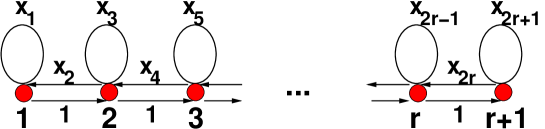
Figure 1. The weighted graph $\Gamma_{r}$, with $r+1$ vertices labeled $1,2,...,r+1$. For each oriented edge $e$, we have indicated the corresponding step weight $w(e)$, namely: $w(i\to i)=x_{2i-1}$ ($i=1,2,...,r+1$), $w(i\to i+1)=x_{2i}$, $w(i+1\to i)=1$ ($i=1,2,...,r$).

For some variables $x_{1},x_{2},...,x_{2r+1}$ elements of a non-commuting algebra, let $J_{1}(x_{1},x_{2},...,x_{2r+1})$ be the “non-commutative Jacobi-type (finite) continued fraction” defined inductively by

$$J_{s}(x_{2s-1},x_{2s},...,x_{2r+1}) = \big{(}1-x_{2s-1}-J_{s+1}(x_{2s+1},x_{2s+2},...,x_{2r+1})x_{2s}\big{)}^{-1}\quad(1\leq s\leq r+1)$$

$$J_{r+2} = 0$$

For some central scalar parameter $t$, the function $J_{1}(tx_{1},...,tx_{2r+1})$, expanded as a formal power series of $t$, may be interpreted combinatorially as the generating series for “quantum” paths on the weighted graph $\Gamma_{r}$ depicted in Fig.1, from and to the origin vertex $1$, each path being weighted by the product of its step weights taken in the order they are traversed and with an extra weight $t$ per step along each edge pointing toward the origin.

Definition 3.1.

To each Motzkin path ${\mathbf{m}}$ we attach a sequence of “weights” ${\mathbf{y}}({\mathbf{m}})=(y_{1}({\mathbf{m}}),...,y_{2r+1}({\mathbf{m}}))$ via the following induction under forward mutation $\mu_{i}^{+}({\mathbf{m}})={\mathbf{m}}^{\prime}$, depending on whether ${\mathbf{m}}$ is in cases (i) or (ii) of Lemma 2.1 above. For short we write $y_{i}({\mathbf{m}})=y_{i}$ and $y_{i}({\mathbf{m}}^{\prime})=y_{i}^{\prime}$. First, we have $y_{j}^{\prime}=y_{j}$ for $j\neq 2i-1,2i,2i+1$ (case (i)) and $j\neq 2i-1,2i,2i+1,2i+2$ (case (ii)), while:

$${\rm\bf Cases\ (i)\ and\ (ii):}\left\{\begin{matrix}y_{2i-1}^{\prime}=y_{2i-1}+y_{2i}\hfill\\ \quad y_{2i}^{\prime}=y_{2i+1}y_{2i}(y_{2i-1}+y_{2i})^{-1}\hfill\\ y_{2i+1}^{\prime}=y_{2i+1}y_{2i-1}(y_{2i-1}+y_{2i})^{-1}\hfill\end{matrix}\right.$$

(3.3) $$\qquad\qquad\ \ {\rm\bf Case(ii):}\ \ \ y_{2i+2}^{\prime}=y_{2i+1}y_{2i-1}(y_{2i-1}+y_{2i})^{-1}$$

This determines the $y$’s entirely in terms of the initial data ${\mathbf{y}}({\mathbf{m}}_{0})$. We have the following Theorems.

Theorem 3.2.

([7]) For the fundamental initial data with ${\mathbf{m}}={\mathbf{m}}_{0}=(0,0,...,0)$, the solution to the quantum $A_{r}$ $Q$-system satisfies the following identity:

(3.4) $$F_{{\mathbf{m}}_{0}}(t)=1+tG_{{\mathbf{m}}_{0}}(t)y_{1}({\mathbf{m}}_{0}),\quad G_{{\mathbf{m}}_{0}}(t)=J_{1}(ty_{1}({\mathbf{m}}_{0}),...,ty_{2r+1}({\mathbf{m}}_{0}))$$

where

(3.5) $$y_{2i-1}({\mathbf{m}}_{0})=R_{i,1}R_{i-1,1}^{-1}R_{i,0}^{-1}R_{i-1,0}\qquad y_{2i}({\mathbf{m}}_{0})=R_{i+1,1}R_{i,1}^{-1}R_{i,0}^{-1}R_{i-1,0}$$

Theorem 3.3.

([7]) For ${\mathbf{y}}({\mathbf{m}}_{0})=(y_{1}({\mathbf{m}}_{0}),...,y_{2r+1}({\mathbf{m}}_{0}))$ given by (3.5), the solution of the recursion (3.3) reads:

(3.6) $$\qquad y_{2i-1}({\mathbf{m}}) = q^{i-1}\,R_{i,m_{i}+1}R_{i,m_{i}}^{-1}R_{i-1,m_{i-1}}R_{i-1,m_{i-1}+1}^{-1}$$

(3.7) $$y_{2i}({\mathbf{m}}) = \left\{\begin{matrix}R_{i+1,m_{i+1}+1}R_{i+1,m_{i+1}}^{-1}R_{i+1,m_{i}}R_{i+1,m_{i}+1}^{-1}&{\rm if}\ m_{i}=m_{i+1}+1\\ {1}&{\rm otherwise}\end{matrix}\right\}$$

$$\times\,R_{i+1,m_{i}+1}R_{i,m_{i}+1}^{-1}R_{i,m_{i}}^{-1}R_{i-1,m_{i}}$$

$$\times\left\{\begin{matrix}R_{i-1,m_{i}+1}R_{i-1,m_{i}}^{-1}R_{i-1,m_{i-1}}R_{i-1,m_{i-1}+1}^{-1}&{\rm if}\ m_{i}=m_{i-1}-1\\ {1}&{\rm otherwise}\end{matrix}\right\}$$

Theorem 3.4.

([7]) For the $y_{i}({\mathbf{m}})$ as in Theorem 3.3, we have:

$$F_{\mathbf{m}}(t)=1+tG_{\mathbf{m}}(t)y_{1}({\mathbf{m}}),\quad G_{\mathbf{m}}(t)=J_{1}({\widehat{y}}_{1}({\mathbf{m}}),...,{\widehat{y}}_{2r+1}({\mathbf{m}}))$$

where ${\widehat{y}}_{i}\equiv{\widehat{y}}_{i}({\mathbf{m}})$ are related to $y_{i}\equiv y_{i}({\mathbf{m}})$ via:

(3.8) $$\left\{\begin{matrix}{\widehat{y}}_{2i-1}=ty_{2i-1}\hfill&{\widehat{y}}_{2i}=ty_{2i}\hfill&{\rm if}\ m_{i+1}=m_{i}\hfill\\ {\widehat{y}}_{2i-1}=t(y_{2i-1}+y_{2i})\hfill&{\widehat{y}}_{2i}=t^{2}y_{2i+1}y_{2i}\hfill&{\rm if}\ m_{i+1}=m_{i}+1\hfill\\ {\widehat{y}}_{2i-1}=ty_{2i-1}-y_{2i+1}^{-1}y_{2i}\hfill&{\widehat{y}}_{2i}=y_{2i+1}^{-1}y_{2i}\hfill&{\rm if}\ m_{i+1}=m_{i}-1\hfill\end{matrix}\right.\qquad(i\in[1,2r+1])$$

Example 3.5.

For ${\mathbf{m}}={\mathbf{m}}_{0}=(0,0,...,0)$, we have ${\widehat{y}}_{i}=ty_{i}$ for $i=1,2,...,2r+1$. The generating function reads

$$G_{{\mathbf{m}}_{0}}(t)=\big{(}1-ty_{1}-t\big{(}1-ty_{3}-t(...(1-ty_{2r-1}-t(1-ty_{2r+1})^{-1}y_{2r})^{-1}...)^{-1}y_{4})^{-1}y_{2}\big{)}^{-1}$$

Example 3.6.

For ${\mathbf{m}}={\mathbf{m}}_{1}=(0,1,...,r-1)$, we have ${\widehat{y}}_{2i-1}=t(y_{2i-1}+y_{2i})$ and ${\widehat{y}}_{2i}=t^{2}y_{2i+1}y_{2i}$ for all $i$, where $y_{i}\equiv y_{i}({\mathbf{m}}_{1})$. The result is simplest for $F_{{\mathbf{m}}_{1}}(t)=1+tG_{{\mathbf{m}}_{1}}(t)y_{1}$. The generating function may be rearranged using the following identity at each step:

(3.9) $$a+b+(1-c-u)^{-1}cb=a+(1-c-u)^{-1}(1-u)b=a+(1-(1-u)^{-1}c)^{-1}b$$

The result reads

$$F_{{\mathbf{m}}_{1}}(t)=\big{(}1-t\big{(}1-t(...(1-t(1-ty_{2r+1})^{-1}y_{2r})^{-1}...)^{-1}y_{2})^{-1}y_{1}\big{)}^{-1}$$

This is easily expressed in terms of the “non-commutative Stieltjes-type (finite) continued fraction” defined inductively as

$$S_{k}(x_{k},x_{k+1},...,x_{2r+1})=(1-S_{k+1}(x_{k+1},...,x_{2r+1})x_{k})^{-1}\ (1\leq k\leq 2r+1),\ S_{2r+2}=1$$

via: $F_{{\mathbf{m}}_{1}}(t)=S_{1}(ty_{1},ty_{2},...,ty_{2r+1})$.

In view of the Example 3.6, we may write another (mixed Stieltjes-Jacobi-type) continued fraction expression for $G_{\mathbf{m}}(t)$ for arbitrary ${\mathbf{m}}$. This will be crucially used in the following.

Any Motzkin path ${\mathbf{m}}=(m_{1},...,m_{r})$ may be decomposed into strictly ascending segments of the form $(m,m+1,...,m+k-1)$ separated by weakly descending steps of the form $(m,m)$ or $(m,m-1)$. Accordingly, we may transform the Jacobi-type fraction for $G_{\mathbf{m}}(t)$ in Theorem 3.4, by “undoing” the pieces of the continued fraction that correspond to the strictly ascending segments of ${\mathbf{m}}$.

To this end, assume that we have a strictly ascending segment $(m_{i_{0}},m_{i_{0}+1},...,m_{i_{0}+k-1})$ with $m_{i_{0}+j}=m_{i_{0}}+j$ for $j=0,1,...,k-1$, which is followed by a weakly decreasing step $(m_{i_{0}+k-1},m_{i_{0}+k})$, with $m_{i_{0}+k}=m_{i_{0}+k-1}$ or $m_{i_{0}+k}=m_{i_{0}+k-1}-1$. Then by definition, we have the relations

$$J_{i_{0}+j} = \big{(}1-t(y_{2i_{0}+2j-1}+y_{2i_{0}+2j})-t^{2}J_{i_{0}+j+1}y_{2i_{0}+2j+1}y_{2i_{0}+2j}\big{)}^{-1}\quad(j\in[0,k-2])$$

(3.10) $$\quad\qquad J_{i_{0}+k-1} = \big{(}1-ty_{2i_{0}+2k-3}-(J_{i_{0}+k}-\delta_{m_{i_{0}+k},m_{i_{0}+k-1}-1}){\widehat{y}}_{2i_{0}+2k-2}\big{)}^{-1}$$

Like in Example 3.5, let us rearrange this piece of fraction iteratively from the bottom up, by using the relation (3.9). This allows to rewrite:

$$J_{i_{0}} = (1-ty_{2i_{0}-1}-tS_{2i_{0}}y_{2i_{0}})^{-1}$$

$$S_{2i_{0}+j} = \big{(}1-tS_{2i_{0}+j+1}y_{2i_{0}+1+j}\big{)}^{-1}\qquad(j\in[0,2k-4])$$

$$S_{2i_{0}+2k-3} = \big{(}1-S_{2i_{0}+2k-2}{\widehat{y}}_{2i_{0}+2k-2}\big{)}^{-1}$$

(3.11) $$S_{2i_{0}+2k-2} = J_{i_{0}+k}-\delta_{m_{i_{0}+k},m_{i_{0}+k-1}-1}$$

Indeed, we start by using (3.9) at the step $j=k-2$ of (3.10), with $a=ty_{2i_{0}+2k-5}$, $b=ty_{2i_{0}+2k-4}$, $c=y_{2i_{0}+2k-3}$ and $u=S_{2i_{0}+2k-2}{\widehat{y}}_{2i_{0}+2k-2}$, to rewrite:

$$J_{i_{0}+k-2}=\Big{(}1-ty_{2i_{0}+2k-5}-t\big{(}1-t(1-S_{2i_{0}+2k-2}{\widehat{y}}_{2i_{0}+2k-2})^{-1}y_{2i_{0}+2k-3}\big{)}^{-1}y_{2i_{0}+2k-4}\Big{)}^{-1}$$

Iterating this leads straightforwardly to (3.11). Repeating this transformation for every strictly ascending segment of ${\mathbf{m}}$, we arrive at:

Theorem 3.7.

For any Motzkin path ${\mathbf{m}}$, we have the following mixed Stieltjes-Jacobi type continued fraction expression for $G_{{\mathbf{m}}}$. Let $i_{1},..,i_{s}$ and $\ell_{1},...,\ell_{s}$ be the positions and lengths of the strictly ascending segments of ${\mathbf{m}}$, of the form $(m_{i_{a}},m_{i_{a}}+1,...,m_{i_{a}+\ell_{a}-1})$, $a=1,2,...,s$. Then we have:

$$G_{\mathbf{m}}(t)= J_{1}$$

$$J_{i}= \big{(}1-{\widehat{y}}_{2i-1}-J_{i+1}{\widehat{y}}_{2i}\big{)}^{-1}\hfill (i\not\in\cup_{a}[i_{a},i_{a}+\ell_{a}-1])$$

$$J_{i_{a}}= \big{(}1-ty_{2i_{a}-1}-S_{2i_{a}}ty_{2i_{a}}\big{)}^{-1}\hfill (a\in[1,s])$$

$$S_{i}= \big{(}1-S_{i+1}ty_{i+1}\big{)}^{-1}\hfill (i\in[2i_{a},2i_{a}+2\ell_{a}-4];a\in[1,s])$$

$$S_{2i_{a}+2\ell_{a}-3}= \big{(}1-S_{2i_{a}+2\ell_{a}-2}{\widehat{y}}_{2i_{a}+2\ell_{a}-2}\big{)}^{-1}\hfill (a\in[1,s])$$

$$S_{2i_{a}+2\ell_{a}-2}= J_{i_{a}+\ell_{a}}-\delta_{m_{i_{a}+\ell_{a}},m_{i_{a}+\ell_{a}-1}-1}\hfill (a\in[1,s])$$

3.3. Quantum commutation relations for the weights

Using the commutations (2.2), we obtain:

Theorem 3.8.

Introducing $p=q^{r+1}$, the weights $y_{i}\equiv y_{i}({\mathbf{m}}_{0})$ of Theorem 3.2 obey the following $p$-commutation relations:

$$y_{i}y_{i+1} = p\,y_{i+1}y_{i}\qquad(i\in[1,2r])$$

$$y_{2i}y_{2i+2} = p\,y_{2i+2}y_{2i}\qquad(i\in[1,r-1])$$

$$y_{j}y_{k} = y_{k}y_{j}\qquad{\rm otherwise}$$

Using the recursion relations (3.3), we deduce the commutation relations of $y_{i}({\mathbf{m}})$, for arbitrary Motzkin paths ${\mathbf{m}}$:

Theorem 3.9.

For a given Motzkin path ${\mathbf{m}}$, the weights $y_{i}\equiv y_{i}({\mathbf{m}})$ have the following commutation relations

(3.12) $$y_{i}y_{i+1} = p\,y_{i+1}y_{i}\qquad(i\in[1,2r])$$

(3.13) $$y_{2i}y_{2i+2} = p^{m_{i}-m_{i+1}+1}\,y_{2i+2}y_{2i}\qquad(i\in[1,r-1])$$

$$y_{j}y_{k} = y_{k}y_{j}\qquad{\rm otherwise}$$

Proof.

By induction under mutation. The Theorem holds for ${\mathbf{m}}={\mathbf{m}}_{0}$ (Theorem 3.8). Assume it holds for some ${\mathbf{m}}$, then consider ${\mathbf{m}}^{\prime}=\mu_{i}^{+}({\mathbf{m}})$ in either cases (i) or (ii) of Lemma 2.1, and denote by $y_{j}^{\prime}\equiv y_{j}({\mathbf{m}}^{\prime})$. We deduce the following commutations from the recursion hypothesis (eq.(3.12)):

(3.14) $$y_{2j-1}y_{2k-1} = y_{2k-1}y_{2j-1}\quad(j,k\in[1,r+1])$$

(3.15) $$(y_{2j-1}+y_{2j})y_{2j+1}y_{2j} = p\,y_{2j+1}y_{2j}(y_{2j-1}+y_{2j})\qquad(j\in[1,r])$$

(3.16) $$(y_{2j-1}+y_{2j})y_{2j+1}y_{2j-1} = y_{2j+1}y_{2j-1}(y_{2j-1}+y_{2j})\qquad(j\in[1,r])$$

In both cases (i) and (ii), this implies that $y_{2j-1}^{\prime}y_{2k-1}^{\prime}=y_{2k-1}^{\prime}y_{2j-1}^{\prime}$ for all $j,k$ and that, as $m_{i-1}=m_{i}$ in both cases, $y_{2i-2}^{\prime}y_{2i-1}^{\prime}=p\,y_{2i-1}^{\prime}y_{2i-2}^{\prime}$, while $y_{2i-1}^{\prime}y_{2i}^{\prime}=p\,y_{2i}^{\prime}y_{2i-1}^{\prime}$ as a consequence of (3.15) and $y_{2i}^{\prime}y_{2i+1}^{\prime}=p\,y_{2i+1}^{\prime}y_{2i}^{\prime}$ by use of (3.15)-(3.16). Finally, we get $y_{2i-2}^{\prime}y_{2i}^{\prime}=y_{2i}^{\prime}y_{2i-2}^{\prime}$ as $y_{2i-2}^{\prime}=y_{2i-2}$ $p$-commutes with both $y_{2i-1}+y_{2i}$ and $y_{2i}$. Using the expressions (3.3) for the cases (i) and (ii), we finally find

• Case (i): $y_{2i}^{\prime}y_{2i+2}^{\prime}=p\,y_{2i+2}^{\prime}y_{2i}^{\prime}$, as $y_{2i+2}^{\prime}=y_{2i+2}$ and $y_{2i}y_{2i+2}=y_{2i+2}y_{2i}$ (from $m_{i+1}=m_{i}+1$).

• Case (ii): $y_{2i}^{\prime}y_{2i+2}^{\prime}=p^{2}\,y_{2i+2}^{\prime}y_{2i}^{\prime}$, as $(y_{2i-1}+y_{2i})$ commutes with $y_{2i+2}y_{2i-1}$ (due to $y_{2i}y_{2i+2}=p\,y_{2i+2}y_{2i}$, from $m_{i+1}=m_{i}$).

Noting finally that $m_{i-1}^{\prime}-m_{i}^{\prime}+1=0$ in both cases (i)-(ii), and that $m_{i}^{\prime}-m_{i+1}^{\prime}+1=1$ in case (i) and $=2$ in case (ii), the Theorem follows. ∎

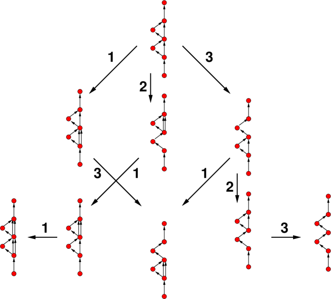
Figure 2. The nine quivers $Q_{\mathbf{m}}$ corresponding to the nine Motzkin paths ${\mathbf{m}}=(m_{1},m_{2},m_{3})\in\mathcal{M}_{3}$, and $Q_{{\mathbf{m}}_{0}=(0,0,0)}$ on top of the diagram. In each quiver, the vertices are all labeled from bottom to top $1,2,...,7$. The arrows between quivers, labeled $i$, correspond to mutations $\mu_{i}^{+}$ in either case (i) or (ii).

To each Motzkin path ${\mathbf{m}}$ we may associate a quiver $Q_{\mathbf{m}}$ with $2r+1$ vertices labelled $i=1,2,...,2r+1$, that summarizes the commutations of the $y_{i}({\mathbf{m}})$’s as follows: we draw $m$ arrows from vertex $i$ to vertex $j$ whenever $y_{i}y_{j}=p^{m}\,y_{j}y_{i}$. For illustration of Theorem 3.9, we have depicted in Fig.2 the example $r=3$ of the quivers $Q_{\mathbf{m}}$ in the fundamental domain $\mathcal{M}_{3}$ of Motzkin paths under global integer translations, and indicated by arrows and superscripts $i$ the mutations $\mu_{i}^{+}$ acting on them.

3.4. Quantum multinomial expressions

3.4.1. $p$-combinatorics

For $a_{1},...,a_{k}\in{\mathbb{Z}}_{+}$, the quantum multinomial coefficient is defined as:

$$\left[\begin{matrix}a_{1}+\cdots+a_{k}\\ a_{1},\ldots,a_{k}\end{matrix}\right]_{p}={\prod_{i=1}^{a_{1}+\cdots+a_{k}}(1-p^{i})\over\prod_{j=1}^{k}\prod_{i=1}^{a_{j}}(1-p^{i})}$$

We assume by convention that when $k=2$, $\left[\begin{matrix}-1\\ 0\end{matrix}\right]_{p}=1$. We have the following $p$-multinomial identity for $k$ variables $x_{1},...,x_{k}$ such that $x_{i}x_{j}=px_{j}x_{i}$ for all $1\leq i<j\leq k$:

$$(x_{1}+\cdots+x_{k})^{n}=\sum_{m_{1},...,,m_{k}\geq 0\atop m_{1}+\cdots m_{k}=n}\left[\begin{matrix}n\\ m_{1},\ldots,m_{k}\end{matrix}\right]_{p}x_{k}^{m_{k}}x_{k-1}^{m_{k-1}}\cdots x_{1}^{m_{1}}$$

This reduces to the standard $p$-binomial identity for $k=2$.

We also define the following formal generating series:

$$\phi_{\ell}(z)=\prod_{i=0}^{\ell-1}(1-p^{i}z)^{-1}=\sum_{m=0}^{\infty}\left[\begin{matrix}\ell+m-1\\ m\end{matrix}\right]_{p}z^{m}$$

and, for variables $x_{1},...,x_{k}$ such that $x_{i}x_{j}=px_{j}x_{i}$ for all $1\leq i<j\leq k$, we have:

$$\phi_{\ell}(x_{1}+\cdots+x_{k})=\sum_{m_{1},\ldots m_{k}\geq 0}\left[\begin{matrix}\ell-1+m_{1}+\cdots+m_{k}\\ \ell-1,m_{1},\ldots,m_{k}\end{matrix}\right]_{p}x_{k}^{m_{k}}x_{k-1}^{m_{k-1}}\cdots x_{1}^{m_{1}}$$

3.4.2. Explicit expressions for $G_{\mathbf{m}}(t)$

We have the following explicit expression for $G_{{\mathbf{m}}_{0}}(t)$, after ordering of the $y_{i}=y_{i}({\mathbf{m}}_{0})$’s.

Theorem 3.10.

For the flat Motzkin path ${\mathbf{m}}_{0}=(0,0,...,0)$, we have:

$$G_{{\mathbf{m}}_{0}}(t) = \sum_{\ell_{1},\ell_{2},...,\ell_{2r+1}\geq 0\atop\ell_{0}=1,\ell_{2r+2}=0}\prod_{i=0}^{r}\left[\begin{matrix}\ell_{2i}+\ell_{2i+1}+\ell_{2i+2}-1\\ \ell_{2i}-1,\ell_{2i+1},\ell_{2i+2}\end{matrix}\right]_{p}(ty_{2r+1})^{\ell_{2r+1}}(ty_{2r})^{\ell_{2r}}\cdots(ty_{1})^{\ell_{1}}$$

$$F_{{\mathbf{m}}_{0}}(t) = 1+\sum_{\ell_{1}\geq 1,\ell_{2},...,\ell_{2r+1}\geq 0\atop\ell_{0}=1,\ell_{2r+2}=0}\prod_{i=0}^{r}\left[\begin{matrix}\ell_{2i}+\ell_{2i+1}+\ell_{2i+2}-1\\ \ell_{2i}-1,\ell_{2i+1},\ell_{2i+2}\end{matrix}\right]_{p}(ty_{2r+1})^{\ell_{2r+1}}(ty_{2r})^{\ell_{2r}}\cdots(ty_{1})^{\ell_{1}}$$

Proof.

By induction. We start with the expression (3.4) for $G_{{\mathbf{m}}_{0}}(t)=J_{1}$, and write the inductive definition $J_{1}=(1-ty_{1}-tJ_{2}y_{2})^{-1}$. Next we note that $y_{1}(J_{2}y_{2})=p(J_{2}y_{2})y_{1}$, as $J_{2}$ only involves $y_{i}$, $i\geq 3$, which all commute with $y_{1}$, by Theorem 3.8. We deduce the formal expansion

$$J_{1}=\sum_{\ell_{1},\ell_{2}\geq 0}\left[\begin{matrix}\ell_{1}+\ell_{2}\\ \ell_{2}\end{matrix}\right]_{p}(tJ_{2}y_{2})^{\ell_{2}}(ty_{1})^{\ell_{1}}$$

Assume we have

(3.17) $$J_{1}=\sum_{\ell_{0},\ell_{1},...,\ell_{2m}\geq 0\atop\ell_{0}=1}\prod_{i=0}^{m-1}\left[\begin{matrix}\ell_{2i}+\ell_{2i+1}+\ell_{2i+2}-1\\ \ell_{2i}-1,\ell_{2i+1},\ell_{2i+2}\end{matrix}\right]_{p}(tJ_{m+1}y_{2m})^{\ell_{2m}}(ty_{2m-1})^{\ell_{2m-1}}\cdots(ty_{1})^{\ell_{1}}$$

for some $m\geq 1$, then by Theorem 3.8, we know that $y_{2m}y_{2m+1}=py_{2m+1}y_{2m}$, $y_{2m}y_{2m+2}=py_{2m+2}y_{2m}$ while $y_{2m}$ commutes with $y_{i}$, $i\geq 2m+3$, and in particular with $J_{m+2}$. This implies:

$$y_{2m}J_{m+1} = y_{2m}(1-ty_{2m+1}-tJ_{m+2}y_{2m+2})^{-1}=(1-pty_{2m+1}-ptJ_{m+2}y_{2m+2})^{-1}y_{2m}$$

$$(tJ_{m+1}y_{2m})^{\ell} = \phi_{\ell}(ty_{2m+1}+tJ_{m+2}y_{2m+2})(ty_{2m})^{\ell}$$

$$= \sum_{\ell_{2m+1},\ell_{2m+2}\geq 0}\left[\begin{matrix}\ell+\ell_{2m+1}+\ell_{2m+2}-1\\ \ell-1,\ell_{2m+1},\ell_{2m+2}\end{matrix}\right]_{p}(tJ_{m+2}y_{2m+2})^{\ell_{2m+2}}(ty_{2m+1})^{\ell_{2m+1}}(ty_{2m})^{\ell}$$

where in the last line we have used the fact that $y_{2m+1}y_{2m+2}=py_{2m+2}y_{2m+1}$, while $y_{2m+1}$ commutes with $J_{m+2}$. Substituting this into (3.17), with $\ell=\ell_{2m}$, we obtain the same summation with $m\to m+1$. We conclude that (3.17) holds for all $m$, and in particular for $m=r+1$, in which case $J_{r+2}=0$ imposes that the last summation reduce to $\ell_{2r+2}=0$, and the first part of the Theorem follows. The second follows trivially from the relation between $F_{{\mathbf{m}}_{0}}$ and $G_{{\mathbf{m}}_{0}}$. ∎

Theorem 3.11.

For the ascending Motzkin path ${\mathbf{m}}_{1}=(0,1,2,...,r-1)$, we have:

$$G_{{\mathbf{m}}_{1}}(t) = \sum_{\ell_{1},\ell_{2},...,\ell_{2r+1}\geq 0}\prod_{i=1}^{2r}\left[\begin{matrix}\ell_{i}+\ell_{i+1}-1+\delta_{i,1}\\ \ell_{i+1}\end{matrix}\right]_{p}(ty_{2r+1})^{\ell_{2r+1}}(ty_{2r})^{\ell_{2r}}\cdots(ty_{1})^{\ell_{1}}$$

$$F_{{\mathbf{m}}_{1}}(t) = \sum_{\ell_{1},\ell_{2},...,\ell_{2r+1}\geq 0}\prod_{i=1}^{2r}\left[\begin{matrix}\ell_{i}+\ell_{i+1}-1\\ \ell_{i+1}\end{matrix}\right]_{p}(ty_{2r+1})^{\ell_{2r+1}}(ty_{2r})^{\ell_{2r}}\cdots(ty_{1})^{\ell_{1}}$$

Proof.

We start from the expression $F_{{\mathbf{m}}_{1}}(t)=S_{1}$ of Example 3.6, and write

$$S_{1}=(1-tS_{2}y_{1})^{-1}=\sum_{\ell_{1}\geq 0}\phi_{\ell_{1}}(tS_{3}y_{2})(ty_{1})^{\ell_{1}}=\sum_{\ell_{1},\ell_{2}\geq 0}\left[\begin{matrix}\ell_{1}+\ell_{2}-1\\ \ell_{2}\end{matrix}\right]_{p}(tS_{3}^{\ell_{2}}y_{2})(ty_{1})^{\ell_{1}}$$

Assume we have

$$S_{1}=\sum_{\ell_{1},...,\ell_{m-1}\geq 0}\prod_{i=1}^{m-2}\left[\begin{matrix}\ell_{i}+\ell_{i+1}-1\\ \ell_{i+1}\end{matrix}\right]_{p}(tS_{m}y_{m-1})^{\ell_{m-1}}(ty_{m-2})^{\ell_{m-2}}\cdots(ty_{1})^{\ell_{1}}$$

for some $m$, then writing $(tS_{m}y_{m-1})^{\ell}=\phi_{\ell}(tS_{m+1}y_{m})y_{m-1}^{\ell}$ immediately implies the same relation for $m\to m+1$. We conclude that it holds for all $m$, in particular for $m=r+2$, where it boils down to the second part of the Theorem. The first part follows from the relation between $F_{{\mathbf{m}}_{1}}$ and $G_{{\mathbf{m}}_{1}}$. ∎

3.4.3. The main Theorem

More generally, we have

Theorem 3.12.

For a generic Motzkin path ${\mathbf{m}}$, we have the following:

$$F_{{\mathbf{m}}}(t) = \sum_{\ell_{1},\ell_{2},...,\ell_{2r+1}\in{\mathbb{Z}}_{+}}A_{\mathbf{m}}(\ell_{1},\ell_{2},...,\ell_{2r+1})(ty_{2r+1})^{\ell_{2r+1}}\cdots(ty_{1})^{\ell_{1}}$$

$$G_{{\mathbf{m}}}(t) = \sum_{\ell_{1},\ell_{2},...,\ell_{2r+1}\in{\mathbb{Z}}_{+}}A_{\mathbf{m}}(\ell_{1}+1,\ell_{2},...,\ell_{2r+1})(ty_{2r+1})^{\ell_{2r+1}}\cdots(ty_{1})^{\ell_{1}}$$

where $A_{\mathbf{m}}$ is defined as the product

$$A_{\mathbf{m}}(\ell_{1},...,\ell_{2k+1}) = \left[\begin{matrix}\ell_{1}+\ell_{2}-1\\ \ell_{2}\end{matrix}\right]_{p}\qquad\raisebox{-14.22636pt}{\hbox{\epsfbox{bottom.eps}}}$$

$$\!\!\!\!\!\!\!\!\!\!\!\!\!\!\!\!\!\!\!\!\!\!\!\!\!\!\!\!\!\!\!\!\!\!\!\!\!\!\!\!\!\!\!\!\!\!\!\!\!\!\!\!\!\!\!\!\times\prod_{i=1}^{r-2}\left\{\begin{matrix}\left[\begin{matrix}\ell_{2i}+\ell_{2i+1}+\ell_{2i+2}-1\\ \ell_{2i}-1,\ell_{2i+1},\ell_{2i+2}\end{matrix}\right]_{p}&{\rm if}\,m_{i+1}=m_{i}&\raisebox{-28.45274pt}{\hbox{\epsfbox{middlea.eps}}}\\ \left[\begin{matrix}\ell_{2i}+\ell_{2i+1}+\ell_{2i+2}-1\\ \ell_{2i}-1\end{matrix}\right]_{p}\left[\begin{matrix}\ell_{2i}+\ell_{2i+1}+\ell_{2i+2}\\ \ell_{2i+2}\end{matrix}\right]_{p}&{\rm if}\,m_{i+1}=m_{i}-1&\raisebox{-28.45274pt}{\hbox{\epsfbox{middleb.eps}}}\\ \left[\begin{matrix}\ell_{2i}+\ell_{2i+1}-1\\ \ell_{2i+1}\end{matrix}\right]_{p}\left[\begin{matrix}\ell_{2i+1}+\ell_{2i+2}-1\\ \ell_{2i+2}\end{matrix}\right]_{p}&{\rm if}\,m_{i+1}=m_{i}+1&\raisebox{-28.45274pt}{\hbox{\epsfbox{middlec.eps}}}\end{matrix}\right\}$$

$$\!\!\!\!\times\left[\begin{matrix}\ell_{2r}+\ell_{2r+1}-1\\ \ell_{2r+1}\end{matrix}\right]_{p}\qquad\raisebox{-14.22636pt}{\hbox{\epsfbox{top.eps}}}$$

where we have represented the local structure of the corresponding quiver $Q_{\mathbf{m}}$ that encodes the $p$-commutations of the $y$’s.

Proof.

As before, we proceed by descending induction. Assume that for some $k\geq 1$, such that $m_{k}=m_{k-1}$ (Case (1)) or $m_{k}=m_{k-1}-1$ (Case (2)), we have an expression of the form:

(3.18) $$F_{{\mathbf{m}}}(t) = \sum_{\ell_{1},...,\ell_{2k}\in{\mathbb{Z}}_{+}}A_{m_{1},...,m_{k}}(\ell_{1},...,\ell_{2k})$$

$$\qquad\times\big{(}(J_{k+1}-\epsilon_{k}){\widehat{y}}_{2k}\big{)}^{\ell_{2k}}(ty_{2k-1})^{\ell_{2k-1}}\cdots(ty_{1})^{\ell_{1}}$$

(3.19) $$\epsilon_{k} = \delta_{m_{k-1},m_{k}+1}$$

We now have three possibilities for the Motzkin path:

Case (a): $m_{k+1}=m_{k}$.

Case (b): $m_{k+1}=m_{k}-1$.

Case (c): $m_{k+j}=m_{k}+j$ for $j=0,1,2,...,\ell-1$ and $m_{\ell}\leq m_{\ell-1}$.

Writing $J_{k+1}=(1-{\widehat{y}}_{2k+1}-J_{k+2}{\widehat{y}}_{2k+2})^{-1}$, we note that we always have ${\widehat{y}}_{2k}{\widehat{y}}_{2k+1}=p{\widehat{y}}_{2k+1}{\widehat{y}}_{2k}$, ${\widehat{y}}_{2k}{\widehat{y}}_{2k+2}=p{\widehat{y}}_{2k+2}{\widehat{y}}_{2k}$, while ${\widehat{y}}_{2k}$ commutes with $J_{k+2}$, as the latter only depends on $y_{i}$ with $i\geq 2k+3$. This allows to write:

$${\rm Case(1)}\!\!: \!\!\!\!(J_{k+1}{\widehat{y}}_{2k})^{m} \!\!\!=\phi_{m}({\widehat{y}}_{2k+1}+J_{k+2}{\widehat{y}}_{2k+2})(ty_{2k})^{m}$$

(3.20) $${\rm Case(2)}\!\!: \!\!\!\!((J_{k+1}-1){\widehat{y}}_{2k})^{m} \!\!\!=p^{m(m-1)\over 2}\phi_{m}({\widehat{y}}_{2k+1}+J_{k+2}{\widehat{y}}_{2k+2})({\widehat{y}}_{2k+1}+J_{k+2}{\widehat{y}}_{2k+2})^{m}({\widehat{y}}_{2k})^{m}$$

$$\!\!\!=\phi_{m}({\widehat{y}}_{2k+1}+J_{k+2}{\widehat{y}}_{2k+2})({\widehat{y}}_{2k+1}+J_{k+2}{\widehat{y}}_{2k+2})^{m}(ty_{2k+1})^{-m}(ty_{2k})^{m}$$

where we have used ${\widehat{y}}_{2k}=ty_{2k}$ in the case (1), and ${\widehat{y}}_{2k}=y_{2k+1}^{-1}y_{2k}$ in the case (2), hence $({\widehat{y}}_{2k})^{m}=p^{-{m(m-1)\over 2}}(ty_{2k+1})^{-m}(ty_{2k})^{m}$.

We first treat the Cases (a) and (b). In both cases, we have $y_{2k+1}{\widehat{y}}_{2k+2}=p\,{\widehat{y}}_{2k+2}y_{2k+1}$, while $y_{2k+1}$ commutes with $J_{k+2}$. This suggests to rewrite

$${\widehat{y}}_{2k+1}+J_{k+2}{\widehat{y}}_{2k+2}=ty_{2k+1}+(J_{k+2}-\epsilon_{k+1}){\widehat{y}}_{2k+2},\qquad\epsilon_{k+1}=\delta_{m_{k+1},m_{k}-1}$$

in which the two summands $p$-commute. In the Cases (1a) and (1b) we get:

$$\phi_{m}(ty_{2k+1}+(J_{k+2}-\epsilon_{k}){\widehat{y}}_{2k+2})=\sum_{j,n\geq 0}\left[\begin{matrix}m-1+j+n\\ m-1,j,n\end{matrix}\right]_{p}((J_{k+2}-\epsilon_{k}){\widehat{y}}_{2k+2})^{n}(ty_{2k+1})^{j}$$

while in the Cases (2a) and (2b):

$$\!\!\!\!\!\!\!\!\!\!\!\!\!\!\!\!\!\!\!\!\!\!\!\!\!\!\!\!\!\!\!\!\!\!\!\!\!\!\!\!\!\!\phi_{m}(ty_{2k+1}+(J_{k+2}-\epsilon_{k}){\widehat{y}}_{2k+2})(ty_{2k+1}+(J_{k+2}-\epsilon_{k}){\widehat{y}}_{2k+2})^{m}$$

$$=\sum_{j\geq 0}\left[\begin{matrix}m-1+j\\ j\end{matrix}\right]_{p}(ty_{2k+1}+(J_{k+2}-\epsilon_{k}){\widehat{y}}_{2k+2})^{m+j}$$

$$=\sum_{j,n\geq 0\atop j+n\geq m}\left[\begin{matrix}j+n-1\\ m-1\end{matrix}\right]_{p}\left[\begin{matrix}j+n\\ j\end{matrix}\right]_{p}((J_{k+2}-\epsilon_{k}){\widehat{y}}_{2k+2})^{n}(ty_{2k+1})^{j}$$

We now deal with the Case (c). By Theorem 3.7, the strictly ascending segment of length $\ell$ starting at $m_{k}$ corresponds to the mixed Stieltjes-Jacobi expression:

$$J_{k+1} = (1-ty_{2k+1}-S_{2k+2}ty_{2k+2})^{-1}$$

$$S_{i} = (1-S_{i+1}ty_{i+1})^{-1}\qquad\qquad(i\in[2k+2,2k+2\ell-2])$$

$$S_{2k+2\ell-1} = (1-(J_{k+\ell+1}-\epsilon_{k+\ell}){\widehat{y}}_{2k+2\ell})^{-1}$$

Eq.(3.20) may be rephrased in the present case by substituting ${\widehat{y}}_{2k+1}+J_{k+2}{\widehat{y}}_{2k}$ with $ty_{2k+1}+S_{2k+2}ty_{2k+2}$. As before the two cases (1) and (2) lead respectively to:

$$\phi_{m}(ty_{2k+1}+(S_{2k+2})ty_{2k+2})=\sum_{j,n\geq 0}\left[\begin{matrix}m-1+j+n\\ m-1,j,n\end{matrix}\right]_{p}(S_{2k+2}ty_{2k+2})^{n}(ty_{2k+1})^{j}$$

$$\phi_{m}(ty_{2k+1}+(S_{2k+2})ty_{2k+2})(ty_{2k+1}+(S_{2k+2})ty_{2k+2})^{m}$$

$$\qquad\qquad\qquad=\sum_{j,n\geq 0\atop j+n\geq m}\left[\begin{matrix}j+n-1\\ m-1\end{matrix}\right]_{p}\left[\begin{matrix}j+n\\ j\end{matrix}\right]_{p}(S_{2k+2}ty_{2k+2})^{n}(ty_{2k+1})^{j}$$

Due to the commutation relations between the $y$’s involved, we may apply directly the recursion in the proof of Theorem 3.11, to get:

$$(S_{2k+2}ty_{2k+2})^{n} = \sum_{\ell_{2k+3},\ell_{2k+4},...,\ell_{2k+2\ell}\geq 0\atop\ell_{2k+2}=n}\prod_{i=2k+2}^{2k+2\ell-1}\left[\begin{matrix}\ell_{i}+\ell_{i+1}-1\\ \ell_{i+1}\end{matrix}\right]_{p}$$

$$\times\ ((J_{k+\ell+1}-\epsilon_{k+\ell}){\widehat{y}}_{2k+2\ell})^{\ell_{2k+2\ell}}(ty_{2k+2\ell-1})^{\ell_{2k+2\ell-1}}\cdots(ty_{2k+3})^{\ell_{2k+3}}(ty_{2k+2})^{n}$$

Assembling all the cases, we find the following recursion relation for $A$ in the cases ($i$a) and ($i$b), with $i=1,2$:

$$A_{m_{1},...,m_{k+1}}(\ell_{1},...,\ell_{2k+2})=A_{m_{1},...,m_{k}}(\ell_{1},...,\ell_{2k})U_{i}(\ell_{2k},\ell_{2k+1},\ell_{2k+2})$$

(3.21) $$\qquad\left\{\begin{matrix}U_{1}=\left[\begin{matrix}\ell_{2k}+\ell_{2k+1}+\ell_{2k+2}-1\\ \ell_{2k}-1,\ell_{2k+1},\ell_{2k+2}\end{matrix}\right]_{p}\\ U_{2}=\left[\begin{matrix}\ell_{2k}+\ell_{2k+1}+\ell_{2k+2}-1\\ \ell_{2k}-1\end{matrix}\right]_{p}\left[\begin{matrix}\ell_{2k}+\ell_{2k+1}+\ell_{2k+2}\\ \ell_{2k+2}\end{matrix}\right]_{p}\end{matrix}\right.$$

and in the cases ($i$c), $i=1,2$:

(3.22) $$\quad A_{m_{1},...,m_{k+\ell-1}}(\ell_{1},...,\ell_{2k+2\ell})$$

$$\qquad\qquad\qquad=A_{m_{1},...,m_{k}}(\ell_{1},...,\ell_{2k})U_{i}(\ell_{2k},\ell_{2k+1},\ell_{2k+2})V(\ell_{2k+2},...,\ell_{2k+2\ell})$$

(3.23) $$\quad V(\ell_{2k+2},...,\ell_{2k+2\ell})=\prod_{i=2k+2}^{2k+2\ell-1}\left[\begin{matrix}\ell_{i}+\ell_{i+1}-1\\ \ell_{i+1}\end{matrix}\right]_{p}$$

This determines $A$ entirely, with the initial conditions:

$${\rm Case\,(a)\,or\,(b)}: A_{m_{1}}(\ell_{1},\ell_{2})= \left[\begin{matrix}\ell_{1}+\ell_{2}-1\\ \ell_{2}\end{matrix}\right]_{p}$$

$${\rm Case(c)}: A_{m_{1},m_{2},...,m_{\ell}}(t)= \prod_{i=1}^{\ell-1}\left[\begin{matrix}\ell_{i}+\ell_{i+1}-1\\ \ell_{i+1}\end{matrix}\right]_{p}$$

and the Theorem follows, with $A_{\mathbf{m}}(\ell_{1},...,\ell_{2r+1})=A_{m_{1},...,m_{r},m_{r}}(\ell_{1},...,\ell_{2r+1},0)$, as the last step has $y_{2r+2}=0$. ∎

Extracting the coefficient of $t^{n}$ in the series of Theorem 3.12, and using the expressions for the weights given by Theorem 3.3, we immediately deduce:

Corollary 3.13.

The solution $R_{1,n}$ of the quantum $A_{r}$ $Q$-system is expressed as a Laurent polynomial of any admissible initial data, with coefficients in ${\mathbb{Z}}_{+}[q,q^{-1}]$.

References

- [1] A. Berenstein, A. Zelevinsky, Quantum Cluster Algebras, Adv. Math. 195 (2005) 405–455. arXiv:math/0404446 [math.QA].
- [2] P. Di Francesco, The solution of the -system with arbitrary boundary, Elec. Jour. of Comb. Vol. 17(1) (2010) R89, arXiv:1002.4427 [math.CO].
- [3] P. Di Francesco and R. Kedem, Q-systems, heaps, paths and cluster positivity, Comm. Math. Phys. 293 No. 3 (2009) 727–802, DOI 10.1007/s00220-009-0947-5. arXiv:0811.3027 [math.CO].
- [4] P. Di Francesco and R. Kedem, -system cluster algebras, paths and total positivity, SIGMA 6 (2010) 014, 36 pages, arXiv:0906.3421 [math.CO].
- [5] P. Di Francesco and R. Kedem, Positivity of the -system cluster algebra, Elec. Jour. of Comb. Vol. 16(1) (2009) R140, Oberwolfach preprint OWP 2009-21, arXiv:0908.3122 [math.CO].
- [6] P. Di Francesco and R. Kedem, Discrete non-commutative integrability: proof of a conjecture by M. Kontsevich, to appear in Int. Math. Res. Notices. arXiv:0909.0615 [math-ph].
- [7] P. Di Francesco and R. Kedem, Noncommutative integrability, paths and quasi-determinants, preprint arXiv:1006.4774 [math-ph].
- [8] S. Fomin and A. Zelevinsky Cluster Algebras I. J. Amer. Math. Soc. 15 (2002), no. 2, 497–529 arXiv:math/0104151 [math.RT].
- [9] R. Kedem, -systems as cluster algebras. J. Phys. A: Math. Theor. 41 (2008) 194011 (14 pages). arXiv:0712.2695 [math.RT].