Explosive behavior in a log-normal interest rate model

Abstract

We consider an interest rate model with log-normally distributed rates in the terminal measure in discrete time. Such models are used in financial practice as parametric versions of the Markov functional model, or as approximations to the log-normal Libor market model. We show that the model has two distinct regimes, at low and high volatility, with different qualitative behavior. The two regimes are separated by a sharp transition, which is similar to a phase transition in condensed matter physics. We study the behavior of the model in the large volatility phase, and discuss the implications of the phase transition for the pricing of interest rates derivatives. In the large volatility phase, certain expectation values and convexity adjustments have an explosive behavior. For sufficiently low volatilities the caplet smile is log-normal to a very good approximation, while in the large volatility phase the model develops a non-trivial caplet skew. The phenomenon discussed here imposes thus an upper limit on the volatilities for which the model behaves as intended.

1 Introduction

An important class of interest rate models used in financial practice is the class of short rate models [1, 15, 25, 7]. These models are Markovian, and the state of the model at time $t$ is completely defined by the short rate $r(t)$. As a result all dynamical variables such as zero coupon bonds and rates at some time $t$ depend only on $r(t)$. These models are simple and intuitive, but have the drawback that the connection between the model parameters and market data is not always transparent. For this reason they are usually not flexible enough in their calibration to market data.

This problem can be solved by the introduction of market models. One particular type of these models are the Markov functional models, where the dynamical quantities of the model are functionals of a small number of Markov drivers $x_{i}(t)$. It has been shown in [14, 15, 1, 2] that by a judicious choice of the functional dependence of some dynamical variable of the model on the stochastic drivers $x_{i}(t)$, it is possible to reproduce exactly Black’s formula or a given market caplet or swaption implied volatility smile.

We consider in this paper a one-factor Markovian model in discrete time with log-normally distributed rates in the terminal measure. Such a model is encountered in practice as a particular parametric realization of a Markov-functional model for simulating an interest rate market with log-normal caplet smile, see e.g. [1]. Models of this type have been proposed in the literature as approximations to the Libor market model with log-normal caplet volatility [6, 19, 8]. For example, the Libor market model reduces to such a model in the frozen drift approximation (up to the addition of appropriate convexity multipliers) when considering only the terminal distribution of the Libors at their setting time. See Sec. 2 for a detailed discussion.

The model with log-normally distributed rates in the terminal measure was studied in Ref. [26], where it was shown that it can be solved exactly for the time-homogeneous case of uniform volatility. Exact results can be found for the dependence of all zero coupon bonds on the Markovian driver. The more general case of a short rate model where the short rate is the exponential of a Gaussian Markov process was considered in [27]. The exact solution of the model was found to have discontinuous dependence on volatility. The main results can be summarized as follows: the model has two distinct regimes, at low and large volatility, respectively, with different qualitative properties. These regimes are separated by a sharp transition, occurring at a critical value of the volatility, which resembles a first order phase transition in condensed matter physics. In particular certain convexity adjustments appearing in the calibration of the model have non-analytic behavior as function of the volatility, manifested as a discontinuous derivative at the critical point.

In this paper we consider the implications of these phenomena for the pricing of interest rates derivatives under such models, and point out that they limit their region of applicability. We start by studying the distributional properties of the Libor probability distribution function in a measure where it is simply related to caplet prices (the forward measure). It turns out that the shape of the Libor distribution function changes suddenly at the critical volatility, and becomes very concentrated at small values of the Libor rates in addition to developing a long tail. This is reflected in Black caplet volatility, which undergoes a sudden change at the critical volatility, both in the ATM volatility and the shape of the caplet smile. While for subcritical volatility the caplet smile is flat to a good approximation, and is equal to the Libor volatility, above the critical volatility the ATM caplet implied volatility increases suddenly, and a nontrivial caplet smile appears. In addition, the moments of the Libor probability distribution function have non-analytic behavior in volatility and explosive behaviour.

Section 2 introduces the model with log-normally distributed rates in the terminal measure which is considered in this paper, and provides some background on the practical relevance of such models. This section gives also a brief review of the main results of [26], describing the method used to find the exact solution of the model, and the main features of the volatility dependence following from this solution. In Section 3 we study the properties of the Libor probability distribution function in the forward measure and its moments, and in Section 4 we consider in some detail the pricing of a Libor payment in arrears, and show the presence of non-analyticity in prices of actual interest rate derivatives in this model. Section 5 gives a summary of the main results, and a brief discussion of their implications.

2 The model

We consider an interest rate model defined on a finite set of dates $t_{i}$

$$0=t_{0}<t_{1}<\cdots<t_{n}\,.$$ (1)

Typically the dates $t_{i}$ are equally spaced, e.g. by 3 or 6 months apart, but we will keep them completely general, and denote the difference between consecutive dates as $\tau_{i}\equiv t_{i+1}-t_{i}$.

The fundamental dynamical quantities of the model are the zero coupon bonds $P_{i,j}\equiv P_{t_{i},t_{j}}$. They are driven by a one-dimensional Markov process $x(t)$, which will be assumed to be a simple Brownian motion under the terminal measure. The numeraire is $P_{t,t_{n}}$, the zero coupon bond maturing at the last simulation time $t_{n}$. Define the forward Libor rate $L_{i}(t)$ for the $(t_{i},t_{i+1})$ period as

$$L_{i}(t)=\frac{1}{\tau_{i}}\Big{(}\frac{P_{t,t_{i}}}{P_{t,t_{i+1}}}-1\Big{)}\,.$$ (2)

The model is defined by the functional dependence on $x(t)$ of the Libor rates at their setting time $L_{i}\equiv L_{i}(t_{i})$. Specifically, in the model considered here the Libors $L_{i}$ are assumed to be log-normally distributed in the terminal measure,

$$L_{i}=\tilde{L}_{i}\exp\Big{(}\psi_{i}x_{i}-\frac{1}{2}\psi_{i}^{2}t_{i}\Big{)}\,.$$ (3)

For simplicity we will denote the value of the Markov driver at time $t_{i}$ as $x_{i}\equiv x(t_{i})$. Its mean and variance are $\mathbb{E}[x_{i}]=0,\mathbb{E}[x_{i}^{2}]=t_{i}$. Here $\psi_{i}$ is the volatility of the Libor $L_{i}$, and $\tilde{L}_{i}$ are parameters which will have be determined such that the initial yield curve $P_{0,i}$ is correctly reproduced.

The original motivation for this work was the study of a Markov-functional model with log-normal functional specification of the Libors at their setting time on the Markovian driver, as given by (3). Such a specification is somewhat different from the original philosophy behind the Markov-functional models [14, 15, 1, 2], which aims to reproduce exactly Black’s formula or model an appropriate market skew for caplets or for swaptions with a judicious choice for the functional dependence $L_{i}(x_{i})$ (or equivalently the functional dependence of the numeraire $P_{t,t_{n}}(x)$). See [18] for a detailed discussion of a specific implementation.

The Markov-functional model is used in practice in parametric and non-parametric versions, according to the implementation of the functional dependence $L_{i}(x_{i})$. The log-normal parametric form considered here is one of the simplest possible, and was considered first in the original work on Markov functional models [14]. For another discussion of this model see Sec. 11.A.2 in [1]. Another parametric version is the so-called semi-parametric representation of Ref. [25]

$$P^{-1}_{i,n}(x)=1+a_{i}e^{b_{i}x}+d_{i}e^{-\frac{1}{2}c_{i}(x-m_{i})^{2}}$$ (4)

where $a_{i},b_{i},c_{i},d_{i},m_{i}$ are numerical parameters to be fitted to the numerical solution. Of course, with a parametric representation the resulting model will not reproduce exactly the caplet or swaption implied volatility for all strikes, and the best one can aim for is to match the implied volatility at one particular strike (for example the ATM point), and possibly also for a region of neighboring strikes.

Models with log-normal rates in the terminal measure appear also when considering approximations to the log-normal Libor market model (LMM) [6]. For a general comparison of the LMM with separable Libor volatility and Markov-functional models in the one-dimensional case see [4]. Consider a model with log-normal caplet volatilities $\psi_{i}$ and given initial yield curve $P_{0,i}$ implying forward Libors $L_{i}^{\rm fwd}=1/\tau_{i}(P_{0,i}/P_{0,i+1}-1)$. A one-factor LMM realization of this model is specified by the diffusion for the forward Libors $L_{i}(t)$ [6]

$$\frac{dL_{i}(t)}{L_{i}(t)}=\psi_{i}dx(t)-\sum_{j=i+1}^{n-1}\frac{\tau_{j}\psi_{j}^{2}L_{j}(t)}{1+L_{j}(t)\tau_{j}}dt$$ (5)

where $x(t)$ is a Brownian motion in the terminal measure. This model is usually simulated using Monte-Carlo methods [1], but several analytical approximations have been proposed as well. The simplest approximation is the frozen drift approximation, where the forward Libors $L_{j}(t)$ in the drift term are replaced with their forward values $L_{j}(0)=L_{j}^{\rm fwd}$. Then the evolution equation can be solved in closed form, and the Libors at their setting time are log-normally distributed in the terminal measure

$$L_{i}^{\rm FD}(t_{i}) = L_{i}^{\rm fwd}\exp\Big{(}\psi_{i}x_{i}-\frac{1}{2}\psi^{2}t_{i}+\mu_{i}t_{i}\Big{)}$$ (6)

$$\mu_{i} = -\sum_{j=i+1}^{n-1}\frac{\tau_{j}\psi_{j}^{2}L_{j}^{\rm fwd}}{1+L_{j}^{\rm fwd}\tau_{j}}$$ (7)

This has the form of (3) with $\tilde{L}_{i}=L_{i}^{\rm fwd}e^{\mu_{i}t_{i}}$. This expression for $\tilde{L}_{i}$ agrees with the small-volatility limit of the convexity-adjusted Libors $\tilde{L}_{i}$ derived in Eq. (27) of [26]. For larger volatilities a convexity adjuster $\kappa_{i}$ must be added to the frozen drift approximation $\tilde{L}_{i}=\kappa_{i}L_{i}^{\rm fwd}e^{\mu_{i}t_{i}}$ such that the yield curve $P_{0,i}$ is correctly reproduced. The frozen drift approximation is expected to be valid only for very small volatility. Improved approximations to the Libor market model which are valid over a larger range of volatilities, and which have log-normally distributed Libors in the terminal measure have been proposed in [19, 8].

This paper presents a study of the model defined by (3) with uniform volatility parameter $\psi_{i}=\psi$, and investigates its properties as functions of the volatility parameter $\psi$. For sufficiently low volatility the model is found to generate a log-normal caplet smile, with caplet volatility equal to $\psi$ to a very good approximation. In retrospect, this provides a justification for the choice of the functional form (3) for describing a model with log-normal caplet volatility. In other words, for sufficiently small caplet volatility, a model with log-normal caplet smile has also log-normally distributed rates in the terminal measure to a very good approximation.

As the volatility parameter $\psi$ is increased, the ATM caplet volatility starts to diverge from the model volatility parameter $\psi$, and a non-trivial caplet smile appears. This change is not gradual, but rather occurs at a sharply defined value of the volatility parameter $\psi_{\rm cr}$, which we call the critical volatility. We will show that at the critical volatility the ATM caplet volatility has a sudden increase, and the shape of the Libor probability distribution in its natural measure changes suddenly from a typical humped shape to a function which is very concentrated near the origin.

Above the critical volatility, the dynamics predicted from the model are different from those intended (log-normal caplet smile), such that this phenomenon introduces a limitation of the model, or more precisely of the choice (3) for the functional dependence of the Libor distribution. In the context of the Libor market model, our results give a measure of the limit of validity of a log-normal approximation. In view of the practical use of this parameterization, it is important to understand its region of applicability.

2.1 Analytical solution

We summarize here the derivation and main features of the analytical solution of the model [26]. The zero coupon bonds $P_{i,j}(x)$ can be expressed as functions of the one-dimensional Markov process $x(t)$. We will denote the numeraire-rebased zero coupon bond prices as $\hat{P}_{i,j}=P_{i,j}/P_{i,n}$. They are martingales in the terminal ($t_{n}$-forward) measure, and thus satisfy the condition, see e.g. [3]

$$\hat{P}_{i,j}=\mathbb{E}_{n}\Big{[}\frac{1}{P_{j,n}}\Big{|}{\cal F}_{i}\Big{]}$$ (8)

Imposing the martingale condition (8) for all possible $i,j$ pairs determines uniquely the convexity-adjusted Libors $\tilde{L}_{i}$, provided that the volatility parameters $\psi_{i}$ are known. The latter are determined for example by calibration to the ATM caplet volatilities, observed in the market.

This model can be solved analytically [26, 27]. For the case of uniform volatility $\psi_{i}=\psi$ the solution can be expressed as an analytical expression for the one-step zero coupon bonds $\hat{P}_{i,i+1}$

$$\hat{P}_{i,i+1}(x_{i})=\sum_{j=0}^{n-i-1}c_{j}^{(i)}e^{j\psi x_{i}-\frac{1}{2}(j\psi)^{2}t_{i}}$$ (9)

with $c_{j}^{(i)}$ a set of constant coefficients to be determined. The convexity-adjusted Libors are given by

$$\tilde{L}_{i}=\frac{\hat{P}_{0,i}-\hat{P}_{0,i+1}}{N_{i}\tau_{i}}\,,$$ (10)

$$N_{i}\equiv\mathbb{E}[\hat{P}_{i,i+1}e^{\psi x_{i}-\frac{1}{2}\psi^{2}t_{i}}]=\sum_{j=0}^{n-i-1}c_{j}^{(i)}e^{j\psi^{2}t_{i}}\,.$$

The coefficients $c_{j}^{(i)}$ satisfy the recursion relation

$$c_{j}^{(i)}=c_{j}^{(i+1)}+\tilde{L}_{i+1}\tau_{i+1}c_{j-1}^{(i+1)}e^{(j-1)\psi^{2}t_{i+1}}$$ (11)

which must be solved simultaneously with Eq. (10) for $\tilde{L}_{i}$. The initial condition is $c_{0}^{(n-1)}=1,\tilde{L}_{n-1}\tau_{n-1}=\hat{P}_{0,n-1}-1$. The recursion relation (11) can be solved backwards in time, for all $i\leq n-1$, finding all coefficients recursively. An explicit solution of this recursion relation was found in [27], and $c_{j}^{(i)}$ has a physical interpretation as the canonical partition function of a one-dimensional attractive Coulomb lattice gas with $j$ particles and $n-i-1$ sites. We will not make use of this solution here, and prefer to evaluate the recursion relation (11) explicitly. The coefficients $c_{j}^{(i)}$ and the convexity-adjusted Libors $\tilde{L}_{i}$ determine the solution of the model. The zero coupon bonds $P_{i,j}$ can be found explicitly as functions of $x=x_{i}$, as shown in Eq. (11).

The recursion relation (11) can be expressed more compactly by introducing the generating function at the time horizon $t_{i}$

$$f^{(i)}(x)\equiv\sum_{j=0}^{n-i-1}c_{j}^{(i)}x^{j}$$ (12)

The generating function $f^{(i)}(x)$ takes known values at $x=0,1$

$$f^{(i)}(0)=1\,,\qquad f^{(i)}(1)=\hat{P}_{0,i+1}$$ (13)

where the second constraint follows from a sum rule for the coefficients $c_{j}^{(i)}$ [26]. The generating function satisfies the recursion relation

$$f^{(i)}(x)=f^{(i+1)}(x)+\tilde{L}_{i+1}\tau xf^{(i+1)}(xe^{\psi^{2}t_{i+1}})$$ (14)

with initial condition $f^{(n-1)}(x)=1$. The expectation value $N_{i}$ appearing in the expression for the convexity-adjusted Libor $\tilde{L}_{i}$ is

$$N_{i}=f^{(i)}(e^{\psi^{2}t_{i}})$$ (15)

The generating function $f^{(i)}(x)$ and thus the coefficients $c_{j}^{(i)}$ can be found in closed form in the two limiting cases of very small and very large volatility $\psi$ [26]. The zero volatility limit of the generating function is

$$f^{(i)}_{0}(x)=\Pi_{j=i+1}^{n-1}(1+L_{j}^{\rm fwd}\tau x)\,.$$ (16)

In the asymptotically large volatility limit $\psi\to\infty$, the recursion relation (14) can be solved again exactly with the result

$$f^{(i)}_{\infty}(x)=1+(\hat{P}_{0,n-1}-1)x+\cdots+(\hat{P}_{0,i+1}-\hat{P}_{0,i+2})x^{n-i-1}\,.$$ (17)

The most distinctive feature of the model in the large volatility limit is an explosive increase of the expectation values $N_{i}=f^{(i)}(e^{\psi^{2}t_{i}})$ with the volatility. This causes the convexity-adjusted Libors $\tilde{L}_{i}$ to become very small. Their asymptotic expression in the large volatility phase is [26]

$$\tilde{L}_{i}=\frac{\hat{P}_{0,i}-\hat{P}_{0,i+1}}{(\hat{P}_{0,i+1}-\hat{P}_{0,i+2})\tau_{i}}e^{-(n-i-1)\psi^{2}t_{i}}(1+O(e^{-\psi^{2}t_{i}}))\,.$$ (18)

In practice $\tilde{L}_{i}$ can become very small, below machine precision, which can make an exact numerical simulation of the model very difficult in the large volatility regime.

2.2 The Libor phase transition

The analytical solution of the model presented above can be used to study exactly its behavior as a function of the volatility parameter $\psi$. It turns out that this is not smooth for all quantities of the model. Certain expectation values, such as $N_{i}$ given in (10), have a $\psi$ dependence which has singular behavior at a special value of volatility which will be called the critical volatility $\psi_{\rm cr}$. This is manifested as a sudden change in the derivative $dN_{i}/d\psi$ at the critical point, which becomes more sharp as the time step $\tau$ decreases, such that it approaches a nonanalyticity point in the continuous time limit [26]. At the critical point the expectation value $N_{i}$ has an explosive increase, which is much faster than in the low volatility phase.

The underlying reason for this phenomenon is a singularity in the generating function $f^{(i)}(x)$ at a certain value $x_{*}$. This value is related to the position of the zeros of $f^{(i)}(x)$ in the complex plane. The generating function is a polynomial in $x$ of degree $n-i-1$ with positive coefficients, and thus does not have any zeros on the positive real axis. It has $n-i-1$ zeros, which are arranged in complex conjugate pairs symmetric with respect to the real axis, along a curve surrounding the origin. The singularity point $x_{*}$ is the point on the positive real axis where the complex zeros pinch the real axis. At this point the derivative of the generating function has a discontinuity which is proportional to the angular density of the zeros around the positive real axis. This density is of the order of $n-i-1$, the number of simulation time steps to the maturity.

This phenomenon is similar to a first order phase transition in condensed matter physics, where the thermodynamical potentials have a discontinuity in the first derivative at the critical point [29]. The analogy becomes even closer in the Lee-Yang formalism of the phase transitions [20], where the critical point is associated with the complex zeros of the grand canonical partition function.

In the context of the Markov functional model with log-normally distributed rates, the singularity in $N_{i}$ occurs at the point $\psi_{\rm cr}$ given by

$$e^{\psi^{2}_{\rm cr}t_{i}}=x_{*}\,.$$ (19)

This equation determines the critical volatility $\psi_{\rm cr}$. A similar phenomenon occurs for any expectation value of the form similar to $N_{i}$

$$\mathbb{E}_{n}[\hat{P}_{i,i+1}e^{\phi x-\frac{1}{2}\phi^{2}t_{i}}]=f^{(i)}(e^{\psi\phi t_{i}})$$ (20)

which can be expressed in terms of the generating function $f^{(i)}(x)$ as shown. The critical volatility corresponding to this expectation value is found in analogy to Eq. (19) and is given by $\exp(\psi\phi t_{i})=x_{*}$.

The precise value of the critical volatility depends on the time step $i$, and on the entire shape of the yield curve $P_{0,i}$. Consider for illustration the case of a constant short rate $r_{0}$, which corresponds to the discount bonds $P_{0,i}=\exp(-r_{0}\tau i)$. A simple estimate of the critical volatility can be obtained from the zeros of the asymptotic generating function $f_{\infty}^{(i)}(x)$, corresponding to very large volatility [26]. Using an approximation for the position of these zeros one finds

$$e^{r_{0}\tau+\psi_{\rm cr}^{2}t_{i}}=\Big{(}\frac{1}{1-e^{-r_{0}\tau}}\Big{)}^{1/(n-i-1)}$$ (21)

which can be approximated, to a good precision, as

$$\psi^{2}_{\rm cr}=\frac{1}{i(n-i-1)\tau}\log\Big{(}\frac{1}{r_{0}\tau}\Big{)}\,.$$ (22)

The relation (22) reproduces the main features of the critical volatility observed in numerical simulations:

• The critical volatility decreases as the size of the time step $\tau$ is reduced, approaching zero in the continuous time limit.

• The critical volatility increases as the short rate $r_{0}$ is reduced, approaching a very large volatility as the rate $r_{0}$ becomes very small.

This behavior is illustrated in Fig. 1. These plots show the critical volatility $\psi_{\rm cr}$ of the model with flat forward short rate $r_{0}$ as function of $\tau$ at fixed $r_{0}$ (left panel), and as function of $r_{0}$ at fixed time step $\tau$ (right panel). In these plots we show both the exact critical volatility (dots/solid lines), which can be found as the value of $\psi$ at which $\partial_{\psi}^{2}\log N_{i}$ is maximal, and the result of the simple approximation (22) (lines/dashed lines). These plots show that the approximation (22) underestimates the actual value of the critical volatility by about 10%.

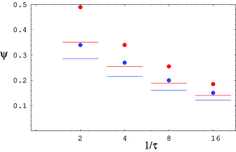
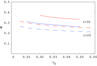
Fig. 1: Left: the critical volatility $\psi_{\rm cr}$ of the log-normal interest rate model with constant forward short rate $r_{0}=5\%$ for several discretizations with $1/\tau=2,4,8,16$ time steps per year. The dots show the exact critical volatility, and the lines the results of the approximation (22). Blue: Libor rate set at $t_{i}=5$, red: Libor rate set at $t_{i}=7.5$. Right: the dependence of the critical volatility $\psi_{\rm cr}(r_{0})$ on the short rate in a simulation with quarterly time steps $\tau=0.25$. The red curves correspond to the Libor rate set at $t_{i}=7.5$ and the blue curves to the Libor rate set at $t_{i}=5$. The solid lines are exact phase boundaries, while the dashed lines correspond to the approximative result Eq. (22). Total simulation time is $t_{n}=10$ years.

3 The Libor probability distribution function

By the model definition (3), the Libor rates $L_{i}$ are log-normally distributed in the $t_{n}$-forward measure (the terminal measure). A more natural measure for pricing instruments depending on the Libor rate $L_{i}$ is the $t_{i+1}$-forward measure (or simply the forward measure), with numeraire the zero-coupon bond $P_{t,i+1}$, maturing at time $t_{i+1}$. We will consider the two measures

$$\mathbb{P}_{n}\,:\quad\,\,\,\,\,\mbox{numeraire }P_{t,n}$$ (23)

$$\mathbb{P}_{i+1}\,:\quad\mbox{numeraire }P_{t,i+1}$$ (24)

As a concrete example, consider a caplet ${\bf C}_{i}(K)$ on the Libor rate $L_{i}=\tau_{i}^{-1}(P_{i,i+1}^{-1}-1)$, set at time $t_{i}$ and paid at time $t_{i+1}$, with strike $K$. The payoff of this instrument is $(L_{i}-K)_{+}$, and its price is given as an expectation value in the $t_{n}$-forward measure $\mathbb{P}_{n}$

$$C_{i}(K)=P_{0,n}\mathbb{E}_{n}[(L_{i}-K)_{+}\hat{P}_{i,i+1}]\,.$$ (25)

Expressed in the forward $\mathbb{P}_{i+1}$ measure, the expression for the caplet price ${\bf C}_{i}(K)$ simplifies and is given by

$$C_{i}(K)=P_{0,i+1}\mathbb{E}_{i+1}[(L_{i}-K)_{+}]$$ (26)

The expectation value in $\mathbb{P}_{i+1}$ measure can be expressed as an integral of the payoff convoluted with the probability distribution function of the Libor $L_{i}$ in this measure. We will denote this distribution $\Phi_{i}(L_{i})$, and we have

$$\mathbb{E}_{i+1}[(L_{i}-K)_{+}]=\int_{0}^{\infty}dL_{i}\Phi_{i}(L_{i})(L_{i}-K)_{+}$$ (27)

In the following we will study in some detail the distribution function $\Phi_{i}(x)$, and its properties. The pdf of the Libor $L_{i}$ in the $\mathbb{P}_{i+1}$ measure can be obtained by comparing Eqs. (25) and (26). It is given by

$$\Phi_{i}(L)=\frac{1}{\hat{P}_{0,i+1}}\frac{e^{-x_{0}^{2}/(2t_{i})}}{\sqrt{2\pi t_{i}}}\frac{1}{\psi L}\hat{P}_{i,i+1}(x_{0})$$ (28)

with $x_{0}=x_{0}(L)$ determined as

$$x_{0}=\frac{1}{\psi}\log\frac{L}{\tilde{L}_{i}}+\frac{1}{2}\psi t_{i}\,.$$ (29)

We would like to study how the Libor probability distribution function $\Phi_{i}(L)$ changes as the volatility $\psi$ is increased from zero to large values. At zero volatility $\psi=0$, this distribution is a delta function concentrated at the forward value

$$\Phi_{i}(L,\psi=0)=\delta(L-L_{i}^{\rm fwd})$$ (30)

As the volatility increases, the distribution widens out. We show in Fig. 2 the shape of the distribution $\Phi_{i}(L)$ for several values of the volatility $\psi$. For moderate values of $\psi$, below the critical volatility $\psi_{\rm cr}$, the distribution has a typical humped shape, peaked around the forward value $L_{i}^{\rm fwd}$.

Above the critical volatility $\psi>\psi_{\rm cr}$ the probability distribution function $\Phi_{i}(L)$ undergoes a dramatic change: its support appears to collapse very rapidly to very small values of $L$, see Fig. 2. The “collapse” of the support of the Libor distribution $\Phi_{i}(L)$ to very small values close to zero is another surprising phenomenon in the high-volatility phase of this model.

Naively, one may ascribe this phenomenon to the fact that the convexity-adjusted Libors $\tilde{L}_{i}$ in the defining equation of the model (3) become very small in the large volatility phase. Upon further reflection the situation is slightly more complicated, for two reasons. First, the log-normal distribution (3) is in the terminal measure $\mathbb{P}_{n}$, while we are interested here in the probability distribution function in $\mathbb{P}_{i+1}$ measure. Second, the martingale condition for $L_{i}(t)$ in $\mathbb{P}_{i+1}$ measure requires that the average of $L_{i}(t_{i})$ should be equal to its forward value $\mathbb{E}_{i+1}[L_{i}]=L_{i}^{\rm fwd}$, which would not be possible if the distribution were concentrated near $L_{i}=0$. The only way for the martingale condition to be satisfied is that the distribution has a long fat tail, which contributes significantly to the average of $L_{i}$.

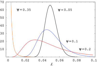
Fig. 2: The probability distribution function $\Phi_{i}(L)$ for the Libor $L_{i}$ in the measure $\mathbb{P}_{i+1}$ for several values of the volatility $\psi$. The plots correspond to a constant forward short rate $r_{0}=5\%$, which gives $L_{i}^{\rm fwd}=5.0314\%$. The remaining parameters are $i=30$, $n=40$, $\tau=0.25$.

In the following we would like to explore this phenomenon in more detail. The analysis presented next will confirm the heuristic arguments mentioned above. We start by showing that the probability distribution function $\Phi_{i}(L)$ can be represented as a sum of log-normal distributions. Define the log-normal distribution with average parameter $\mu$ and dispersion $\sigma$

$$\phi(x;\mu,\sigma)=\frac{1}{x\sqrt{2\pi}\sigma}e^{-\frac{1}{2\sigma^{2}}(\log x-\mu)^{2}}$$ (31)

The $j$-th moment of the $x$ variable under the distribution $\phi(x;\mu,\sigma)$ is

$$\mathbb{E}[x^{j}]=e^{j\mu+\frac{1}{2}j^{2}\sigma^{2}}$$ (32)

The probability distribution function of the $L_{i}$ Libor in the $\mathbb{P}_{i+1}$ measure (28) can be represented as a sum of log-normal distributions with different averages but the same variance

$$\Phi_{i}(L)=\frac{1}{\hat{P}_{0,i+1}}\sum_{j=0}^{n-i-1}c_{j}^{(i)}\phi(L;\mu_{j}^{(i)},\sigma_{i}=\psi\sqrt{t_{i}})$$ (33)

where

$$\mu_{j}^{(i)}=\log\Big{(}\tilde{L}_{i}e^{(j-\frac{1}{2})\psi^{2}t_{i}}\Big{)}\,.$$ (34)

The average value of $L$ under the log-normal distribution $\phi(L;\mu_{j}^{(i)},\sigma_{i}=\psi\sqrt{t_{i}})$ is

$$\mathbb{E}[L|\phi(L;\mu_{j}^{(i)},\sigma_{i})]=\tilde{L}_{i}e^{j\psi^{2}t_{i}}$$ (35)

so each of these log-normal distributions are peaked at successively higher values of $L$. Specifically, the pdf of the Libor (33) consists of a sum of log-normal distributions with averages $\tilde{L}_{i},\tilde{L}_{i}e^{\psi^{2}t_{i}},\cdots,\tilde{L}_{i}e^{(n-i-1)\psi^{2}t_{i}}$, and weights $c_{k}^{(i)}/\hat{P}_{0,i+1}$ with $k=0,1,\cdots,n-i-1$. We recall that the weights add up to 1 due to the exact sum rule $\sum_{j=0}^{n-i-1}c_{j}^{(i)}=\hat{P}_{0,i+1}$.

The weights $c_{j}^{(i)}/\hat{P}_{0,i+1}$ of the terms with $j>1$ decrease sufficiently fast with $j$, such that the total average of $L$ is equal to the forward Libor rate, as required by the martingale condition for $L_{i}$ in the $\mathbb{P}_{i+1}$ measure

$$\mathbb{E}_{i+1}[L] = \frac{1}{\hat{P}_{0,i+1}}\sum_{j=0}^{n-i-1}c_{j}^{(i)}\mathbb{E}[L|\phi(L;\mu_{j}^{(i)},\sigma_{i})]$$

$$= \frac{1}{\hat{P}_{0,i+1}}\sum_{j=0}^{n-i-1}c_{j}^{(i)}\tilde{L}_{i}e^{j\psi^{2}t_{i}}=L_{i}^{\rm fwd}\,.$$

The representation (33) of the distribution function can be used to obtain a qualitative understanding of the behavior of this function in the large volatility limit $\psi^{2}t_{i}\gg 1$. In this limit the asymptotic behavior of the convexity adjusted Libors $\tilde{L}_{i}$ is given by (18). In the large volatility regime, the convexity adjusted Libors decrease very rapidly with the volatility $\psi$. This means that most of the log-normal components of the distribution function $\Phi_{i}(L)$ have vanishingly small averages, except for the last one with the largest index $j=n-i-1$

$$\mathbb{E}[L|\phi(L;\mu_{j}^{(i)},\sigma_{i})] = L_{i}^{\rm max}e^{-(n-i-1-j)\psi^{2}t_{i}}\,,$$ (37)

where

$$L_{i}^{\rm max}=\frac{\hat{P}_{0,i}-\hat{P}_{0,i+1}}{(\hat{P}_{0,i+1}-\hat{P}_{0,i+2})\tau_{i}}=L_{i}^{\rm fwd}\frac{1+L_{i+1}^{\rm fwd}\tau_{i+1}}{L_{i+1}^{\rm fwd}\tau_{i+1}}\,.$$ (38)

For typical values of model parameters, such as $L^{\rm fwd}=5\%,\tau=0.25$, one has $L^{\rm max}\sim 500\%$ which is a very large value compared to typical rates.

In the large volatility regime the coefficients $c_{j}^{(i)}$ are all comparable, such that the shape of the probability distribution function $\Phi_{i}(L)$ is expected to be very concentrated near $L=0$, corresponding to the terms with $j=0,1,\cdots,n-i-2$, and to have a fat tail extending to very large values of $L\sim L^{\rm max}$, corresponding to the term with $j=n-i-1$. This is confirmed by direct calculation of the distribution function in the large volatility limit, as observed in Fig. 2.

The behavior of the Libor probability distribution function in the $\mathbb{P}_{i+1}$ measure in the large volatility limit is related to a numerical issue discussed in [26], which is responsible for the unobservability of the phase transition in usual simulation methods such as Monte Carlo or finite difference methods. This numerical issue appears in the calculation of the expectation value (10) as an integral

$$N_{i}=\mathbb{E}[\hat{P}_{i,i+1}e^{\psi x-\frac{1}{2}\psi^{2}t_{i}}]=\int_{-\infty}^{\infty}\frac{dx}{\sqrt{2\pi t_{i}}}e^{-\frac{x^{2}}{2t_{i}}}\hat{P}_{i,i+1}(x)e^{\psi x-\frac{1}{2}\psi^{2}t_{i}}\,.$$ (39)

At volatilities above the critical value $\psi>\psi_{\rm cr}$ the integrand in this expression develops a secondary peak at a relatively large value of $|x|\sim 10\sqrt{t_{i}}$, in addition to the peak around $x\sim 0$, see Fig. 4 in [26]. The secondary peak gives the dominant contribution to the integral in the large volatility limit. However, the region of large $x$ where it appears is either very poorly sampled, or completely ignored in usual simulation methods, which thus will fail to take it into account.

The dominance of the integral by the secondary peak in the super-critical regime can be understood by changing variables in the integral (39) from $x$ to $L_{i}$, the Libor rate. We observe that the integrand of (39) is simply related to the Libor probability distribution function $\Phi_{i}(L)$ in the $\mathbb{P}_{i+1}$ measure, when expressed in terms of $x=x(L)$ given in Eq. (29). The integral in (39) becomes, after changing the integration variable from $x$ to $L$

$$N_{i}=\hat{P}_{0,i+1}\int_{0}^{\infty}dL\Phi_{i}(L)\frac{L}{\tilde{L}_{i}}\,.$$ (40)

The secondary peak in the integrand of (39) becomes the fat tail of $\Phi_{i}(L)$, while the peak near $x\sim 0$ corresponds to the region of $L\sim\tilde{L}_{i}$. As discussed above, the fat tail of $\Phi_{i}(L)$ is essential in order for the integral above to reproduce correctly its non-arbitrage value; the counterpart of this statement in the $x-$integral (39) is that the secondary peak is also required by the consistency of the model, and can not be neglected.

3.1 The moments of the Libor pdf

In this section we consider the moments of the Libor probability distribution function $\Phi_{i}(L)$ in the forward $\mathbb{P}_{i+1}$ measure. We will show that its moments, and thus its characteristic function

$$\tilde{\Phi}_{i}(u) = \int_{-\infty}^{\infty}dLe^{iuL}\Phi_{i}(L)=\sum_{j=0}^{\infty}\frac{(iu)^{j}}{j!}\mathbb{E}_{i+1}[L_{i}^{j}]$$ (41)

can be expressed in terms of the generating function $f^{(i)}(x)$.

The moments of $\Phi_{i}(L)$ can be computed using Eq. (33). The integral can be performed straightforwardly by changing the integration variable from $L$ to $x$. The result expresses the $j-$th moment of the Libor distribution in the forward measure in terms of the generating function $f^{(i)}(x)$ as

$$M_{j}=\mathbb{E}_{i+1}[L_{i}^{j}] = \int_{0}^{\infty}dL_{i}(L_{i})^{j}\Phi_{i}(L_{i})=\frac{1}{\hat{P}_{0,i+1}}{\tilde{L}_{i}}^{j}e^{\frac{1}{2}j(j-1)\psi^{2}t_{i}}f^{(i)}(e^{j\psi^{2}t_{i}})\,.$$ (42)

We consider a few particular cases of the relation Eq. (42). The first two moments $j=0,1$ do not contain dynamical information, and are constrained by general considerations as follows. The $j=0$ moment is the normalization integral, and is indeed equal to 1 by the condition (13)

$$M_{0}=\frac{1}{\hat{P}_{0,i+1}}f^{(i)}(1)=1\,.$$ (43)

The first moment can be found again in closed form, and is equal to the forward Libor rate $L_{i}^{\rm fwd}$, as expected

$$M_{1}=\frac{1}{\hat{P}_{0,i+1}}\tilde{L}_{i}f^{(i)}(e^{\psi^{2}t_{i}})=\frac{\hat{P}_{0,i}-\hat{P}_{0,i+1}}{\hat{P}_{0,i+1}\tau_{i}}=L_{i}^{\rm fwd}\,.$$ (44)

This expresses the martingale condition for $L_{i}$ in the $\mathbb{P}_{i+1}$ measure.

More interesting is the result for the second moment $M_{2}$. This determines the equivalent lognormal volatility of the Libor rate $L_{i}$ as

$$\sigma_{\rm LN}^{2}t_{i}=\log\Big{(}\frac{M_{2}}{M_{1}^{2}}\Big{)}=\log\Big{(}\hat{P}_{0,i+1}e^{\psi^{2}t_{i}}\frac{f^{(i)}(e^{2\psi^{2}t_{i}})}{[f^{(i)}(e^{\psi^{2}t_{i}})]^{2}}\Big{)}$$ (45)

In the small volatility limit $\psi^{2}t_{i}\ll 1$ the ratio of generating functions can be computed using the approximative formula (16). This gives

$$\sigma_{LN}^{2}=\psi^{2}(1+O(\psi^{2}t_{i}))\,.$$ (46)

This means that in the small volatility limit the caplet log-normal volatilities are approximately equal to $\psi$. This is useful for the calibration of the model, as the $\psi_{i}$ volatilities can be read off directly from ATM caplet volatilities.

When considered as a function of the volatility $\psi$, the moments $M_{j},j\geq 2$ of the Libor probability distribution function $\Phi_{i}(L)$ have non-analytic dependence on $\psi$ at a value of the volatility $\psi_{\rm cr}^{(j)}$ given by the solution to the equation

$$x_{*}(\psi)=e^{j\psi^{2}t_{i}}$$ (47)

where $x_{*}(\psi)$ is the non-analyticity point of the generating function $f^{(i)}(x)$ at time horizon $t_{i}$. This is the point on the real positive axis where the complex zeros of the generating function $f^{(i)}(x)$ pinch the real axis. In general the position of the non-analyticity point $x_{*}(\psi)$ depends on the volatility parameter $\psi$, although it approaches a well-defined value in the very large volatility limit $\psi\to\infty$, when the generating function approaches the asymptotic expression $f_{\infty}^{(i)}(x)$ given in Eq. (17). The zeros and the non-analyticity point of the polynomial $f_{\infty}^{(i)}(x)$ have been studied in detail in [26] for the case of a constant forward short rate. As discussed above, approximating the generating function with its asymptotic expression $f_{\infty}^{(i)}(x)$ leads to the result (21) for the critical volatility.

Assuming that $x_{*}(\psi)$ is independent on $\psi$ (as is the case for asymptotically large volatility), from (47) it follows that the critical volatilities of the moments of the Libor distribution function are related as

$$\psi_{\rm cr}^{(j)}=\frac{\psi_{\rm cr}}{\sqrt{j}}\,,\quad\psi\to\infty$$ (48)

However, in reality the non-analyticity point occurs at moderate values of the volatility $\psi$, for which $x_{*}$ has a pronounced dependence on $\psi$. This implies that the simple relation (48) is badly violated in practice.

We illustrate the non-analyticity in volatility of the moments $M_{j}$ on the example of the second moment $M_{2}$. This is the most important moment from a practical point of view, as it determines the Black log-normal caplet volatility according to Eq. (45). In Figure 4 we show a plot of the equivalent Black caplet volatility $\sigma_{\rm LN}$ as a function of $\psi$ (red curve) at the time horizon $i=30$ in a simulation with $n=40$ quarterly time steps.

The equivalent log-normal volatility $\sigma_{\rm LN}$ has two turning points, at $\psi$ around 0.3 and at 0.33. The critical point at the time horizon considered here is $\psi_{\rm cr}=0.33$, which corresponds to the second point. In order to understand the first turning point, we show in the Appendix the zeros of the generating function $f^{(i)}(x)$ together with two circles of radius $e^{\psi^{2}t_{i}}$ and $e^{2\psi^{2}t_{i}}$. From these plots one can see that the first turning point coincides with the zeros crossing the larger circle of radius $e^{2\psi^{2}t_{i}}$, and the second turning point corresponds to the volatility $\psi$ at which the zeros cross the smaller circle, of radius $e^{\psi^{2}t_{i}}$. Since the position of the zeros changes with $\psi$, the first turning point (the critical volatility of the second moment $M_{2}$) $\psi_{\rm cr}^{(2)}=0.3$ differs from the large volatility limit prediction following from Eq. (48) $\psi_{\rm cr}/\sqrt{2}\simeq 0.23$, obtained by assuming stationary zeros. This illustrates the comment made above about the limited validity of Eq. (48).

Only the first few moments have non-analyticity points. The reason for this is that at very low volatilities $\psi$, the zeros of the generating function do not surround completely the origin, but a gap remains between the real axis and the zeros. As the volatility increases, the zeros move closer to the origin, and close together onto the real axis. However, at this point they have crossed already the circles of radii $e^{j\psi^{2}t_{i}}$, with $j>j_{0}$ such that the moments $M_{j}$ do not have a non-analyticity point for sufficiently large $j>j_{0}$. In other words, the equation (47) does not have a solution for sufficiently large index $j$. The maximal index $j_{0}$ of the moment of the Libor pdf $L_{i}$ which still has a phase transition depends on the time horizon $t_{i}$ considered.

The price of an instrument which is sensitive to the $j-$th moment will have a non-analyticity point at the corresponding value of the volatility. For the second moment this is the case for example with the Libor payment in arrears, discussed in the next section.

3.2 Caplet pricing and Black caplet volatility

A closed form expression for the caplet price can be found by direct evaluation of the expectation value in (25)

$$C_{i}(K)=P_{0,n}\sum_{j=0}^{n-i-1}c_{j}^{(i)}[\tilde{L}_{i}e^{j\psi^{2}t_{i}}N(f_{1})-KN(f_{2})]$$ (49)

with

$$f_{1} = -\frac{1}{\sqrt{t_{i}}}[x_{0}(K)-(j+1)\psi t_{i}]$$ (50)

$$f_{2} = -\frac{1}{\sqrt{t_{i}}}[x_{0}(K)-j\psi t_{i}]$$ (51)

$$x_{0}(K) = \frac{1}{\psi}\log\frac{K}{\tilde{L}_{i}}+\frac{1}{2}\psi t_{i}\,.$$ (52)

This has the typical form of a mixing solution [21, 22] for an option price on an asset with a probability distribution consisting of a superposition of log-normal distributions.

Figure 3 shows typical results for the Black (log-normal) caplet volatility $\sigma_{\rm BS}(K)$ for several values of the volatility $\psi$, obtained from the exact formula (49). At low values of $\psi$ the Black volatility is independent of strike, which means that the distribution $\Phi_{i}(L)$ is aproximatively log-normal. In Figure 4 we show a plot of the exact ATM Black caplet volatility for ATM strike $K=5\%$. From this plot one can see that, for small $\psi$, the ATM caplet volatility is to a very good approximation equal to $\psi$. This agrees with the prediction (45), and confirms that for sufficiently small volatility, the Libor volatility parameter $\psi$ is equal to a very good approximation with the caplet volatility. At larger values of $\psi$ above the critical volatility $\psi_{\rm cr}=0.33$, the smile is not flat, which signals deviations from a log-normal distribution for $\Phi_{i}(L)$.

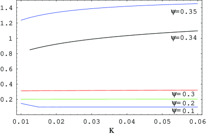
Fig. 3: Implied caplet volatility smile $\sigma_{\rm BS}(K)$ for several values of the volatility $\psi$, as function of the strike $K$. The caplet is defined on the rate $L_{30}$ in a simulation with $n=40$ time steps, $\tau=0.25$ and constant forward short rate $r_{0}=5\%$. The forward Libor is $L_{i}^{\rm fwd}=5.0\%$.

In Figure 4 we show also the ATM equivalent Black caplet volatility $\sigma_{\rm LN}$ given by Eq. (45) (red curve), comparing it with the exact ATM caplet volatility $\sigma_{\rm BS}$ (black curve). The critical volatility corresponding to the caplet shown in this plot is $\psi_{\rm cr}=0.33$. We observe that the exact and approximative volatilities agree with each other for small $\psi$, where they satisfy very well the approximative equality relation (46). This region is the intended region of applicability of the model.

As the volatility $\psi$ is increased, a sharp turn in the equivalent volatility $\sigma_{\rm LN}$ occurs at $\psi_{\rm cr}^{(2)}\sim 0.3$, which corresponds to the critical volatility of the second moment of the Libor distribution function, as explained above. The second turn point is at $\psi_{\rm cr}=0.33$ which is the critical volatility of the model at the maturity $t_{i}$ considered. It is interesting that for $\psi>\psi_{\rm cr}$ the equivalent log-normal volatility decreases as the model volatility $\psi$ increases.

The exact ATM caplet volatility has a first turning point which is closer to the critical volatility $\psi_{\rm cr}=0.33$. It starts to diverge from the equivalent log-normal volatility $\sigma_{\rm LN}$ at a lower volatility $\psi\sim 0.3$, which thus is the point where the shape of the Libor distribution function starts to deviate appreciably from a log-normal shape. The fast increase in the ATM caplet volatility above the critical volatility is explained by the appearance of the long tail of the Libor distribution function $\Phi_{i}(L)$ extending to very large values of $L$. This gives a large contribution to the caplet price, which is given by a simple integral over $\Phi_{i}(L)$

$$C_{i}(K)=P_{0,i+1}\int_{0}^{\infty}dL(L-K)_{+}\Phi_{i}(L)\,.$$ (53)

We remarked above on the numerical importance of the tail of the $\Phi_{i}(L)$ distribution in relation to the integral (40), where it is needed in order for this integral to reproduce its non-arbitrage value. Based on the same argument, one expects that the tail of this distribution will contribute significantly also to the caplet price $C_{i}(K)$ above the critical point.

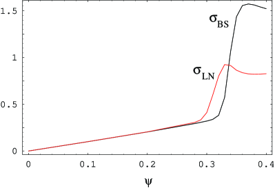
Fig. 4: The exact ATM caplet volatility $\sigma_{\rm BS}$ (black), and the equivalent log-normal caplet volatility $\sigma_{\rm LN}$ computed using (45) (red), as functions of the volatility parameter $\psi$. The caplet strike is $K=5\%$, the forward Libor is $L^{\rm fwd}=5.0\%$, corresponding to a constant forward short rate $r_{0}=5\%$. The remaining model parameters are $i=30$, $n=40$, $\tau=0.25$.

4 Libor payment in arrears

We consider in this section the pricing of a Libor payment in arrears in the model with log-normally distributed rates in the terminal measure. We derive the convexity adjustment, and compare it with the known convexity adjustment in the model with log-normal caplet volatility. It will be seen that the convexity adjustment in the model with log-normally distributed rates in the terminal measure has a phase transition at two values of the Libor volatility, in contrast to the latter, which is perfectly well-behaved as function of the caplet volatility.

The Libor payment in arrears pays the amount $L_{i}\tau_{i}$ at time $t_{i}$, where $L_{i}$ is the Libor rate for the $(t_{i},t_{i+1})$ period, set at $t_{i}$. The price of this instrument in the terminal measure is

$$A_{i} = P_{0,n}\mathbb{E}_{n}[L_{i}(x_{i})\tau_{i}P_{i,n}^{-1}(x_{i})]=P_{0,n}\mathbb{E}_{n}[L_{i}(x_{i})\tau_{i}\hat{P}_{i,i+1}(x_{i})(1+L_{i}(x_{i})\tau_{i})]\,.$$ (54)

The first term, linear in $L_{i}$, is known exactly from the pricing of a forward rate agreement

$$\mathbb{E}_{n}[L_{i}(x_{i})\tau_{i}\hat{P}_{i,i+1}(x_{i})] = \hat{P}_{0,i}-\hat{P}_{0,i+1}=P_{0,i+1}(L_{i}^{\rm fwd}\tau_{i})\,.$$ (55)

The only non-trivial part is the pricing of the term quadratic in $L_{i}$, which can be expressed in terms of the generating function

$$\mathbb{E}_{n}[L^{2}_{i}(x_{i})\hat{P}_{i,i+1}(x_{i})]=\tilde{L}_{i}^{2}e^{\psi^{2}t_{i}}f^{(i)}(e^{2\psi^{2}t_{i}})$$ (56)

Recall that the convexity-adjusted Libor is given by

$$\tilde{L}_{i}=\frac{\hat{P}_{0,i}-\hat{P}_{0,i+1}}{f^{(i)}(e^{\psi^{2}t_{i}})\tau_{i}}=\hat{P}_{0,i+1}L_{i}^{\rm fwd}\frac{1}{f^{(i)}(e^{\psi^{2}t_{i}})}$$ (57)

Combining all the pieces together we get for the price of a Libor payment in arrears

$$\frac{A_{i}}{P_{0,i+1}} = (L_{i}^{\rm fwd}\tau_{i})+\hat{P}_{0,i+1}(L_{i}^{\rm fwd}\tau_{i})^{2}e^{\psi^{2}t_{i}}\frac{f^{(i)}(e^{2\psi^{2}t_{i}})}{[f^{(i)}(e^{\psi^{2}t_{i}})]^{2}}\,.$$ (58)

The second term is the convexity adjustment, and can be expressed in terms of the equivalent log-normal volatility $\sigma_{\rm LN}$ introduced above in (45). We obtain the following result for the price of a Libor payment in arrears in the model with log-normally distributed Libors in the terminal measure

$$A_{i}=P_{0,i+1}(L_{i}^{\rm fwd}\tau_{i})\Big{\{}1+(L_{i}^{\rm fwd}\tau_{i})e^{\sigma_{LN}^{2}t_{i}}\Big{\}}\,.$$ (59)

This can be compared with the exact result for the price of a Libor payment in arrears in a model with exact log-normal caplet volatility $\psi$ for the Libor $L_{i}$

$$A_{i}=P_{0,i+1}(L_{i}^{\rm fwd}\tau_{i})\Big{\{}1+(L_{i}^{\rm fwd}\tau_{i})e^{\psi^{2}t_{i}}\Big{\}}$$ (60)

This model has a log-normal Libor distribution function in the measure $\mathbb{P}_{i+1}$. The result (60) is identical with the price in the model with log-normal Libor in the terminal measure $\mathbb{P}_{n}$ (59), up to the replacement $\sigma_{\rm LN}\to\psi$.

At low volatility $\psi$, the equivalent volatility $\sigma_{\rm LN}$ is approximatively equal to $\psi$, see Eq. (46). For larger volatility $\psi$ it has a more complex behavior as discussed in Sec. 3.1, including two non-analyticity points at $\psi_{\rm cr}^{(2)}$ and $\psi_{\rm cr}$, as observed in Fig. 4. This means that the price of this instrument has the same non-analytical behavior in $\psi$ as $\sigma_{\rm LN}(\psi)$.

Similar non-analyticity effects can be expected to appear in the pricing of other interest rates derivatives, and are introduced either through non-analytic behavior in the convexity-adjusted Libors $\tilde{L}_{i}$, or through the moments of the Libor distribution function in the forward measure $\mathbb{P}_{i+1}$. Thus non-analyticity effects appear to be a generic feature of models with log-normally distributed rates in the terminal measure.

5 Conclusions

We considered in this paper the dynamics of an interest rate model with log-normally distributed rates in the terminal measure. Such models are used in financial practice as particular parametric realizations of the Markov functional model, and as approximations to models with log-normal caplet smile, such as the log-normal Libor market model. Using the exact solution of the model we studied the dependence on volatility of the distributional properties of the dynamical quantities of the model and their implications for pricing interest rate derivatives. The main result of the study is the existence of a previously unobserved sharp transition at a critical value of the volatility. Above the critical volatility certain expectation values and convexity adjustments have an explosive growth. The values of the critical volatility in simulations with 10-30y and interest rates around 5% are comparable with actual log-normal caplet volatilities observed in the market, such that the existence of this phase transition is of practical relevance, and imposes a limit on the applicability of the model.

It has been long known that models with log-normally distributed rates suffer from singular behavior. This was observed in [12, 28] in the context of the Dothan model, and of the Black-Karasinski model. However, the phenomenon discussed here appears to be different in several respects: first, the singularity discussed in [12, 28] was shown to appear for a continuous time model, while the model considered here is defined in discrete time. Second, the transition discussed here appears at a well-defined finite value of the volatility, while the divergence studied in [12, 28] is independent of volatility.

The results of this paper show that at low volatilities a log-normal caplet smile can be well reproduced by assuming Libor log-normality in the terminal measure; however at larger volatility this property is not preserved, and a non-trivial cap smile is generated. These results spell out the limits of applicability of the log-normal parameterization (3) for describing an interest rate market with log-normal caplet smile. Such models can be applied only for sufficiently low caplet volatility, below the critical volatility.

The underlying reason for this limitation is a change in the shape of the probability distribution function of the Libor rates in their forward measure around the critical volatility. For small volatility the Libor pdf has a typical humped shape, centered around the forward Libor value. However, at the critical volatility this pdf changes suddenly, and it collapses to small Libor values, in addition to developing a long tail. Furthermore, the moments of this probability distribution function have also sharp transitions as functions of volatility.

Fig. 5: The position of the zeros of the generating function $f^{(i)}(x)$ for several values of the volatility $\psi=0.3-0.33$ at the time horizon $i=30$ in a simulation with $n=40$ quarterly time steps ($\tau=0.25$). The two circles shown have radii $e^{\psi^{2}t_{i}}$ and $e^{2\psi^{2}t_{i}}$. The zeros cross these circles at $\psi_{\rm cr}$ and $\psi^{(2)}_{\rm cr}$, corresponding to the critical volatility of the model, and to the critical volatility of the second moment of the Libor distribution function, respectively.

These phenomena have implications for interest rate derivative pricing under the given model, and we considered as concrete examples caplets on Libor rates and Libor payments in arrears. The caplet prices, the Black caplet volatilities, and the convexity adjustment for Libor payments in arrears display also sharp transitions as functions of the model volatility. Based on these examples, it is plausible to expect that this phenomenon occurs also for other interest rate derivatives, and is a general feature of the interest rates models with log-normally distributed rates in the terminal measure.

The effects discussed in this paper are due to a contributions to the expectation values from a region in the state variable (Markovian driver) which is usually assumed to be unimportant in practice, as it is associated with very large interest rates $\sim 100\%$. This region is usually truncated off in tree and finite difference simulations, or is very poorly sampled in Monte Carlo simulations, unless extremely high numbers of paths are used. This implies that usual numerical implementations of this model do not capture correctly the behavior of the model in the large volatility phase, and thus the phase transition is not visible under these simulation methods. In practice one can take the view that the implementation version of the model with its built-in limitations (e.g. limits on the range of the Markovian driver $x(t)$) is the model. This corresponds to a truncation of the original model, and the numerical consistency of this truncation must be carefully verified.

The arguments of this paper are limited to the time-homogeneous setting of a uniform volatility, but it is plausible that a similar phenomenon will occur also in the practically relevant but analytically more complex case of time-dependent volatility $\psi_{i}$. This is confirmed by the study of a related model in [27], where the stochastic driver $x(t)$ is replaced with an Ornstein-Uhlenbeck process. This corresponds to the Black-Karasinski model in the terminal measure, with mean reversion and term structure of caplet volatilities. The exact solution of this model obtained in [27] shows the presence of a similar phase transition in volatility in the convexity adjustments of the model. Finally, it would be interesting to investigate whether some of these results persist also in a model with exact log-normal caplet volatility, such as the exact Markov functional model [2, 14] or the Libor market model [6]. This is plausible in view of the result obtained in [10], according to which the Libor distribution function in the terminal measure in the LMM has log-normal tails, which is similar to the distributional property (3) of the model considered here.

Acknowledgements. I am grateful to Emanuel Derman and the participants at the Columbia University IEOR seminar for comments and discussions, and to an anonymous referee for useful comments and criticism. The information, views and opinions set forth in this publication are those of the author, and are in no ways sponsored, endorsed, or related to the business of J. P. Morgan Chase & Co. (“J. P. Morgan”). J. P. Morgan does not warrant the publication’s completeness or accuracy, and makes no representations regarding the use of the information set forth in this publication. In no event shall J. P. Morgan be liable for any direct, indirect, special, punitive, or consequential damages, including loss of principal and/or lost profits, even if notified of the possibility of such damages. Nothing in this publication is intended to be an advertisement or offer for any J. P. Morgan service.

Appendix

We illustrate in this Appendix the relation between the position of the zeros of the generating function $f^{(i)}(x)$ and the non-analyticity properties of the moments of the Libor distribution function discussed in Sec. 3.1. We take as a concrete example a simulation with $n=40$ quarterly time steps, with constant forward short rate $r_{0}=5\%$, and we examine the zeros of the $f^{(i)}(x)$ at the time step $i=30$.

The plots in Fig. 5 show the movement of the zeros of $f^{(30)}(x)$ as a function of the volatility $\psi$ for $\psi=0.3-0.33$. On the same plots are shown also two circles with radii $e^{\psi^{2}t_{i}}$ and $e^{2\psi^{2}t_{i}}$. The values of the volatility at which the zeros cross these circles are the critical volatility $\psi_{\rm cr}$ and the critical volatility of the second moment $\psi_{\rm cr}^{(2)}$, respectively. These critical volatilities are visible as turning points in the plot of the equivalent log-normal volatility $\sigma_{\rm LN}$ as function of $\psi$ in Fig. 4.

A similar picture holds for the higher order moments. For example, the $j$-th moment of the Libor distribution function $M_{j}=\mathbb{E}_{i+1}[L_{i}^{j}]$ will have a non-analyticity point at $\psi_{\rm cr}^{(i)}$. This corresponds to that value of the volatility where the zeros of $f^{(i)}(x)$ cross the circle of radius $e^{j\psi^{2}t_{i}}$. As mentioned in the text, for sufficiently high order moments the zeros do not surround completely the origin, and these moments will not have a phase transition.

References

- [1] L. Andersen and V. Piterbarg, Interest Rate Modeling, Atlantic Financial Press, 2010.
- [2] P. Balland and L. P. Hughston, Markov Market Model Consistent with Cap Smile, Int. J. Th. Appl. Finance, 3, 161-181 (2000).
- [3] M. Baxter and A. Rennie, Financial calculus: An introduction to derivative pricing, Cambridge University Press, 1996.
- [4] M. Bennett and J. Kennedy, A comparison of Markov-functional and market models: the one-dimensional case, The Journal of Derivatives 13, 22-43 (2005).
- [5] F. Black, E. Derman and W. Toy, A One-Factor Model of Interest Rates and Its Application to Treasury Bond Options, Financial Analysts Journal 24-32 (1990).
- [6] A. Brace, D. Gatarek and M. Musiela, The market model of interest rate dynamics, Math. Finance 7, 125-155 (1997).
- [7] D. Brigo and F. Mercurio, Interest Rate Models - Theory and Practice: With Smile, Inflation and Credit, Springer Verlag 2006.
- [8] A. Daniluk and D. Gatarek, A fully lognormal Libor market model, Risk 18(9), 115-118, Sept. 2005.
- [9] L. U. Dothan, On the Term Structure of Interest Rates, Journal of Financial Economics 6, 59-69 (1978).
- [10] S. Gerhold, Moment explosion in the Libor market model, Statistics and Probability Letters 81, 560-562 (2011), arXiv:1008.2104[q-fin.PR]
- [11] P. Glasserman and X. Zhao, Arbitrage free discretization of log-normal forward Libor and swap rate models, Finance and Stochastics 4, 35-68 (2000)
- [12] M. Hogan and K. Weintraub, The lognormal interest rate model and eurodollar futures, Citibank working paper, 1993.
- [13] Z. Hu, J. Kerkhof, P. McCloud and J. Wackertapp, Cutting edges using domain integration, Risk, 95, 2006.
- [14] P. Hunt, J. Kennedy and A. Pellser, Markov-Functional Interest Rate Models, Finance and Stochastics, 4, 391-408 (2000).
- [15] J. B. Hunt and J. E. Kennedy, Financial Derivatives in Theory and Practice, Wiley Series in Probability and Statistics, 2005.
- [16] F. Jamshidian, Forward Induction and Construction of Yield Curve Diffusion Models, J. Fixed Income 1, 62-74 (1991).
- [17] F. Jamshidian, Libor and swap markets models and measures, Finance and Stochastics 1, 293-330 (1997).
- [18] S. Johnson, Numerical methods for the Markov-functional models, Wilmott, 68 (2006).
- [19] O. Kurbanmuradov, K. Sabelfeld and J. Schoenmakers, Lognormal approximations to Libor market models, Journal of Computational Finance 6(1), 69-100, 2002.
- [20] T. D. Lee and C. N. Yang, Statistical Theory of Equations of State and Phase Transitions. II. Lattice Gas and Ising Model, Physical Review Letters 87, 410-419 (1952); Phys. Rev. 87, 410 (1952).
- [21] A. L. Lewis, Option Valuation under Stochastic Volatility: with Mathematica Code, Finance Press, Newport Beach, 2000.
- [22] A. L. Lewis, The Mixing Approach to Stochastic Volatility and Jump Models, 2002.
- [23] K. Miltersen, L. Sandmann and D. Sondermann, Closed Form Solutions for Term Structure Derivatives with Log-normal Interest Rates, J. Finance 52, 409-430 (1997).
- [24] M. Musiela and M. Rutkowski, Martingale methods in financial modeling, Springer-Verlag (1997).
- [25] A. Pelsser, Efficient Methods for Valuing Interest Rate Derivatives, Springer Finance, 2000.
- [26] D. Pirjol, Phase Transition in a Log-normal Markov Functional Model, J. Math. Phys. 52, 013301 (2011), arXiv:1007.0691 [q-fin].
- [27] D. Pirjol, Equivalence of Interest Rate Models and Lattice Gases, Phys. Rev. E 85, 046116 (2012), arXiv:1204.0915 [q-fin].
- [28] K. Sandmann and D. Sondermann, A note on the stability of lognormal interest rate models and the pricing of Eurodollar futures, Mathematical Finance 7(2), 119-125 (1997).
- [29] E. H. Stanley, Introduction to Phase Transitions and Critical Phenomena, Oxford University Press, 1987.