A general fractional
porous medium equation

Abstract

We develop a theory of existence and uniqueness for the following porous medium equation with fractional diffusion,

$$\left\{\begin{array}[]{ll}\dfrac{\partial u}{\partial t}+(-\Delta)^{\sigma/2}(|u|^{m-1}u)=0,&\qquad x\in\mathbb{R}^{N},\;t>0,\\[8.0pt] u(x,0)=f(x),&\qquad x\in\mathbb{R}^{N}.\end{array}\right.$$

We consider data $f\in L^{1}(\mathbb{R}^{N})$ and all exponents $0<\sigma<2$ and $m>0$. Existence and uniqueness of a weak solution is established for $m>m_{*}=(N-\sigma)_{+}/N$, giving rise to an $L^{1}$-contraction semigroup. In addition, we obtain the main qualitative properties of these solutions. In the lower range $0<m\leq m_{*}$ existence and uniqueness of solutions with good properties happen under some restrictions, and the properties are different from the case above $m_{*}$. We also study the dependence of solutions on $f,m$ and $\sigma$. Moreover, we consider the above questions for the problem posed in a bounded domain.

2000 Mathematics Subject Classification. 26A33, 35A05, 35K55, 76S05
Keywords and phrases. Nonlinear fractional diffusion, nonlocal diffusion operators, porous medium equation.

1 Introduction

The aim of this paper is to develop a theory of existence and uniqueness, as well as to obtain the main qualitative properties, for a family of nonlinear fractional diffusion equations of porous medium type. More specifically, we consider the Cauchy problem

(1.1) $$\left\{\begin{array}[]{ll}\dfrac{\partial u}{\partial t}+(-\Delta)^{\sigma/2}(|u|^{m-1}u)=0,&\qquad x\in\mathbb{R}^{N},\;t>0,\\[11.38109pt] u(x,0)=f(x),&\qquad x\in\mathbb{R}^{N}.\end{array}\right.$$

We take initial data $f\in L^{1}(\mathbb{R}^{N})$, which is a standard assumption in diffusion problems, with no sign restriction. As for the exponents, we consider the fractional exponent range $0<\sigma<2$, and take porous medium exponent $m>0$. In the limit $\sigma\to 2$ we recover the standard Porous Medium Equation (PME)

$$\dfrac{\partial u}{\partial t}-\Delta(|u|^{m-1}u)=0,$$

which is a basic model for nonlinear and degenerate diffusion, having now a well-established theory [39].

The nonlocal operator $(-\Delta)^{\sigma/2}$, known as the Laplacian of order $\sigma$, is defined for any function $g$ in the Schwartz class through the Fourier transform: if $(-\Delta)^{\sigma/2}g=h$, then

(1.2) $$\widehat{h}\,(\xi)=|\xi|^{\sigma}\,\widehat{g}(\xi).$$

If $0<\sigma<2$, we can also use the representation by means of an hypersingular kernel,

(1.3) $$(-\Delta)^{\sigma/2}g(x)=C_{N,\sigma}\mbox{ P.V.}\int_{\mathbb{R}^{N}}\frac{g(x)-g(z)}{|x-z|^{N+{\sigma}}}\,dz,$$

where $C_{N,\sigma}=\frac{2^{\sigma-1}\sigma\Gamma((N+\sigma)/2)}{\pi^{N/2}\Gamma(1-\sigma/2)}$ is a normalization constant, see for example [30]. There is another classical way of defining the fractional powers of a linear self-adjoint nonnegative operator, in terms of the associated semigroup, which in our case reads

(1.4) $$(-\Delta)^{\sigma/2}g(x)=\frac{1}{\Gamma(-\frac{\sigma}{2})}\int_{0}^{\infty}\left(e^{t\Delta}g(x)-g(x)\right)\frac{dt}{t^{1+\frac{\sigma}{2}}}.$$

It is easy to check that the symbol of this operator is again $|\xi|^{\sigma}$. The advantage of this approach is that it gives a natural way of defining the problem in a bounded domain, by means of the spectral characterization of the semigroup $e^{t\Delta}$, see [38]. The problem posed in a bounded domain is also studied in this paper.

Equations of the form (1.1) can be seen as fractional-diffusion versions of the PME. Though our paper is aimed at providing a sound mathematical theory for this evolution equation and the nonlinear semigroups generated by Problem (1.1) and the problem posed on bounded domains, we mention that the equation appears as a model in statistical mechanics [26], and the linear counterpart in [27]. We also want to point out that there are other natural options of nonlinear, possibly degenerate fractional-diffusion evolutions under current investigation. Thus, the papers [14], [15] consider the following fractional diffusion PME   $\partial_{t}u-\nabla\cdot(u\nabla(-\Delta)^{-s/2}u)=0$. It has very different properties from the ones we derive for (1.1). The standard PME (with $m=2$) is recovered in such model for $s=0$. A more detailed discussion on these issues is contained in the survey paper [40].

These two kinds of equations can be also viewed as nonlinear versions of the linear fractional diffusion equation obtained for $m=1$, which has the integral representation

(1.5) $$u(x,t)=\int_{\mathbb{R}^{N}}K_{\sigma}(x-z,t)f(z)\,dz,$$

where $K_{\sigma}$ has Fourier transform $\widehat{K}_{\sigma}(\xi,t)=e^{-|\xi|^{\sigma}t}$. This means that, for $0<\sigma<2$, the kernel $K_{\sigma}$ has the form $K_{\sigma}(x,t)=t^{-N/\sigma}F(|x|\,t^{-1/\sigma})$ for some profile function $F$ that is positive and decreasing, and behaves at infinity like $F(r)\sim r^{-(N+\sigma)}$ [9]. When $\sigma=1$, $F$ is explicit; if $\sigma=2$ the function $K_{2}$ is the Gaussian heat kernel. The linear model has been well studied by probabilists, since the fractional Laplacians of order $\sigma$ are infinitesimal generators of stable Lévy processes [1], [7]. However, an integral representation of the evolution like (1.5) is not available in the nonlinear case, thus motivating our work.

In a previous article [35] we studied Problem (1.1) for the particular case $\sigma=1$. The key tool there was the well-known representation of the half-Laplacian in terms of the Dirichlet-Neumann operator, which allowed us to formulate the nonlocal problem in terms of a local one (i. e., involving only derivatives and not integral operators). For $\sigma\neq 1$, Caffarelli and Silvestre [13] have recently given a similar characterization of the Laplacian of order $\sigma$ in terms of the so-called $\sigma$-harmonic extension, which is the solution of an elliptic problem with a degenerate or singular weight. However, even with this local characterization at hand, many of the proofs that we gave for $\sigma=1$ cannot be adapted to cope with a general $\sigma$. Hence we have needed to use new tools, which in several cases do not involve the extension. These techniques, which include some new functional inequalities, have also allowed us to improve the results obtained in [35] for the case $\sigma=1$. The case of a bounded domain was not treated in that paper.

2 Main results

As in the case of the PME, there is a unified theory of existence and uniqueness of a suitable concept of weak solution above a critical exponent, given for a general $\sigma\in(0,2)$ by $m_{*}\equiv(N-\sigma)_{+}/N$. The linear case $m=1$ lies always in this range.

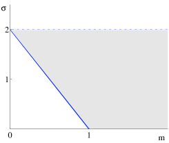
Figure 1: The critical line $m_{*}=(N-\sigma)/N$ and the supercritical region $m>m_{*}$ for $N\geq 3$, $N=2$, and $N=1$.

  Theorem 2.1

Let $m>m_{*}$ and $\sigma\in(0,2)$. For every $f\in L^{1}(\mathbb{R}^{N})$ there exists a unique weak solution of Problem (1.1).

The precise definition of weak solution that guarantees uniqueness is stated in Definition 3.1 or equivalently in Definition 3.2.

The construction of the solution in the previous theorem follows from a double limit procedure, approximating first the initial datum by a sequence of bounded functions, and also approximating $\mathbb{R}^{N}$ by a sequence of bounded domains with null boundary data. In this respect we show existence of a weak solution to the associated Cauchy-Dirichlet problem, a result that has an independent interest, see Section 4.

The weak solutions to Problem (1.1) have some nice qualitative properties that are summarized as follows.

  Theorem 2.2

Assume the hypotheses of Theorem 2.1, and let $u$ be the weak solution to Problem (1.1).

• $\partial_{t}u\in L^{\infty}((\tau,\infty):L^{1}(\mathbb{R}^{N}))$ for every $\tau>0$.

• Mass is conserved: $\int_{\mathbb{R}^{N}}u(x,t)\,dx=\int_{\mathbb{R}^{N}}f(x)\,dx$ for all $t\geq 0$.

• Let $u_{1},u_{2}$ be the weak solutions to Problem (1.1) with initial data $f_{1},f_{2}\in L^{1}(\mathbb{R}^{N})$. Then,

  $$\int_{\mathbb{R}^{N}}(u_{1}-u_{2})_{+}(x,t)\,dx\leq\int_{\mathbb{R}^{N}}(f_{1}-f_{2})_{+}(x)\,dx,\ \text{\emph{($L^{1}$-order-contraction property)}}.$$

• Any $L^{p}$-norm of the solution, $1\leq p\leq\infty$, is non-increasing in time.

• The solution is bounded in $\mathbb{R}^{N}\times[\tau,\infty)$ for every $\tau>0$ ($L^{1}$-$L^{\infty}$ smoothing effect). Moreover, for all $p\geq 1$,

  (2.1) $$\|u(\cdot,t)\|_{L^{\infty}(\mathbb{R}^{N})}\leq C\,t^{-\gamma_{p}}\|f\|_{L^{p}(\mathbb{R}^{N})}^{\delta_{p}},$$

  with $\gamma_{p}=(m-1+{\sigma}p/N)^{-1}$, $\delta_{p}=\sigma p\gamma_{p}/N$, and  $C=C(m,p,N,\sigma)$.

• If $f\geq 0$ the solution is positive for all $x$ and all positive times.

• If either $m\geq 1$ or $f\geq 0$, then $u\in C^{\alpha}(\mathbb{R}^{N}\times(0,\infty))$ for some $0<\alpha<1$.

• The solution depends continuously on the parameters $\sigma\in(0,2)$, $m>m_{*}$, and $f\in L^{1}(\mathbb{R}^{N})$ in the norm of the space $C([0,\infty):\,L^{1}(\mathbb{R}^{N}))$.

Remarks. (a) Properties (i) and (ii) were only known for $\sigma=1$ in the case of nonnegative initial data [35].

(b) The positivity property (vi) is not true for the PME in the range $m>1$. The fact that it holds for Problem (1.1) stems from the nonlocal character of the diffusion operator.

(c) A weak solution satisfying property (i) is said to be a strong solution, see Definition 6.1. These kind of solutions satisfy the equation in (1.1) almost everywhere in $Q=\mathbb{R}^{N}\times(0,\infty)$.

Our main interest in this paper is in describing the theory in the above mentioned range $m>m_{*}$. However, we also consider the lower range $0<m\leq m_{*}$ for contrast. In that range (which implies that $0<\sigma<1$ if $N=1$) we obtain existence if we restrict the data class (or if we relax the concept of solution). In addition, in order to have uniqueness, we need to ask the solution to be strong.

  Theorem 2.3

Let $\sigma\in(0,2)$ and $0<m\leq m_{*}$. For every $f\in L^{1}(\mathbb{R}^{N})\cap L^{p}(\mathbb{R}^{N})$ with $p>p_{*}(m)=(1-m)N/\sigma$ there exists a unique strong solution to Problem (1.1).

Figure 2: The critical line $p_{*}=(1-m)N/\sigma$ and the existence region of strong solutions.

This theorem improves the results obtained of [35] for $\sigma=1$, since in that paper existence and uniqueness of a (weak) solution were only proved for the case of integrable and bounded initial data, $f\in L^{1}(\mathbb{R}^{N})\cap L^{\infty}(\mathbb{R}^{N})$. Moreover, the weak solution was only proved to be strong in the case of nonnegative initial data.

Some of the properties of the solutions in this lower range are rather different from those in the upper range.

  Theorem 2.4

Assume the hypotheses of Theorem 2.3, and let $u$ be the strong solution to Problem (1.1).

• The mass $\int_{\mathbb{R}^{N}}u(x,t)\,dx$ is conserved if $m=m_{*}$. Mass is not conserved if $m<m_{*}$. Actually, when $0<m<m_{*}$ there is a finite time $T>0$ such that $u(x,T)\equiv 0$ in $\mathbb{R}^{N}$.

• There is an $L^{1}$-order-contraction property.

• Any $L^{p}$-norm of the solution, $1\leq p\leq\infty$, is non-increasing in time.

• The solution is bounded in $\mathbb{R}^{N}\times[\tau,\infty)$ for every $\tau>0$ ($L^{p}$-$L^{\infty}$ smoothing effect). Moreover, if $p>p_{*}(m)$ (which is necessary to make $\gamma_{p}>0$) then formula (2.1) holds.

• If $f\geq 0$ the solution is positive for all $x$ and all positive times up to the extinction time.

• Let $f\geq 0$ and let $T$ be the extinction time. Then $u\in C^{\alpha}(\mathbb{R}^{N}\times(0,T))$ for some $0<\alpha<1$.

We will make a series of comments on these two results. First, we point out that the result on the conservation of mass for $m=m_{*}$ is new even for $\sigma=1$.

A more essential observation is that there is an alternative approach: using the results of Crandall and Pierre [22] we can obtain the existence of a unique so-called mild solution for all $f\in L^{1}(\mathbb{R}^{N})$ in the whole range of $m$ and $\sigma$, via the abstract theory of accretive operators. This approach has therefore the advantage of having general scope. Two problems arise with this way of looking at the problem: (a) how to characterize the mild solution in differential terms; and (b) how to derive its properties. Our paper answers both questions.

The strong solutions that we have constructed are mild solutions. Hence, in our restricted range of initial data the unique mild solution is a strong solution. For a general $f\in L^{1}(\mathbb{R}^{N})$ and $m\leq m_{*}$, we will show that the mild solution is a very weak solution (a solution in the sense of distributions), see Theorem 8.4. However, we will fail to prove that this very weak solution is a weak solution in the sense of Definition 3.1, and hence we will not be able to obtain the properties listed above (bit note that the $L^{1}$-contraction holds since it is a consequence of the accretivity of the operator).

As to the continuous dependence of the solution in terms of the parameters, convergence in $L^{1}(\mathbb{R}^{N})$ is not expected to hold for $0<m<m_{*}$, since mass is not conserved in that region. Instead we expect to have continuity in weighted spaces, much in the spirit of [5]. Nevertheless, we are able to extend the continuous dependence result of Theorem 2.2-(viii) to cover the case $m=m_{*}$ for $N>2$, see Proposition 10.1. We also show that continuity holds in the upper limit $\sigma\to 2$, thus recovering the standard PME, see Theorem 10.2.

3 Weak solutions. An equivalent problem

3.1 Weak solutions

If $\psi$ and $\varphi$ belong to the Schwartz class, Definition (1.2) of the fractional Laplacian together with Plancherel’s theorem yield

(3.1) $$\int_{\mathbb{R}^{N}}(-\Delta)^{\sigma/2}\psi\,\varphi=\int_{\mathbb{R}^{N}}|\xi|^{\sigma}\hat{\psi}\,\hat{\varphi}=\int_{\mathbb{R}^{N}}|\xi|^{\sigma/2}\hat{\psi}|\xi|^{\sigma/2}\,\hat{\varphi}=\int_{\mathbb{R}^{N}}(-\Delta)^{\sigma/4}\psi\,(-\Delta)^{\sigma/4}\varphi.$$

Therefore, if we multiply the equation in (1.1) by a test function $\varphi$ and integrate by parts, as usual, we obtain

(3.2) $$\int_{0}^{\infty}\int_{\mathbb{R}^{N}}u\dfrac{\partial\varphi}{\partial t}\,dxds-\int_{0}^{\infty}\int_{\mathbb{R}^{N}}(-\Delta)^{\sigma/4}(|u|^{m-1}u)(-\Delta)^{\sigma/4}\varphi\,dxds=0.$$

This identity will be the basis of our definition of a weak solution.

The integrals in (3.2) make sense if $u$ and $|u|^{m-1}u$ belong to suitable spaces. The correct space for $|u|^{m-1}u$ is the fractional Sobolev space $\dot{H}^{\sigma/2}(\mathbb{R}^{N})$, defined as the completion of $C_{0}^{\infty}(\mathbb{R}^{N})$ with the norm

$$\|\psi\|_{\dot{H}^{\sigma/2}}=\left(\int_{\mathbb{R}^{N}}|\xi|^{\sigma}|\hat{\psi}|^{2}\,d\xi\right)^{1/2}=\|(-\Delta)^{\sigma/4}\psi\|_{2}.$$

  Definition 3.1

A function $u$ is a weak ($L^{1}$-energy solution) to Problem (1.1) if:

• $u\in C([0,\infty):L^{1}(\mathbb{R}^{N}))$, $|u|^{m-1}u\in L^{2}_{\rm loc}((0,\infty):\dot{H}^{\sigma/2}(\mathbb{R}^{N}))$;

• identity (3.2) holds for every $\varphi\in C_{0}^{1}(\mathbb{R}^{N}\times(0,\infty))$;

• $u(\cdot,0)=f$ almost everywhere.

For brevity we will call weak solutions the solutions obtained below according to this definition, but the complete name weak $L^{1}$-energy solution is used in the statement to recall that we are making a very definite choice.

The main disadvantage in using this definition is that there is no formula for the fractional Laplacian of a product, or of a composition of functions. Moreover, there is no benefit in using compactly supported test functions since their fractional Laplacian loses this property. To overcome these difficulties, we will use the fact that our solution $u$ is the trace of the solution of a local problem obtained by extending $|u|^{m-1}u$ to a half-space whose boundary is our original space.

3.2 Extension Method

If $g=g(x)$ is a smooth bounded function defined in $\mathbb{R}^{N}$, its $\sigma$-harmonic extension to the upper half-space, $v=\mathop{\rm E}(g)$, is the unique smooth bounded solution $v=v(x,y)$ to

(3.3) $$\left\{\begin{array}[]{ll}\nabla\cdot(y^{1-\sigma}\nabla v)=0,&\text{in }\mathbb{R}^{N+1}_{+}\equiv\{(x,y)\in\mathbb{R}^{N+1}:x\in\mathbb{R}^{N},y>0\},\\ v(x,0)=g(x),&x\in\mathbb{R}^{N}.\end{array}\right.$$

Then, Caffarelli and Silvestre [13] proved that

(3.4) $$-\mu_{\sigma}\lim_{y\to 0^{+}}y^{1-\sigma}\frac{\partial v}{\partial y}=(-\Delta)^{\sigma/2}g(x),\quad\mu_{\sigma}={2^{\sigma-1}\Gamma(\sigma/2)}/{\Gamma(1-\sigma/2)}.$$

In (3.3) the operator $\nabla$ acts in all $(x,y)$ variables, while in (3.4) $(-\Delta)^{\sigma/2}$ acts only on the $x=(x_{1},\cdots,x_{N})$ variables. In the sequel we denote

$$L_{\sigma}v\equiv\nabla\cdot(y^{1-\sigma}\nabla v),\qquad\dfrac{\partial v}{\partial y^{\sigma}}\equiv\mu_{\sigma}\lim_{y\to 0^{+}}y^{1-\sigma}\frac{\partial v}{\partial y}.$$

Operators like $L_{\sigma}$, with a coefficient $y^{1-\sigma}$, which belongs to the Muckenhoupt space of weights $A_{2}$ if $0<\sigma<2$, have been studied by Fabes et al. in [24]. We make use of this theory later in the proof of positivity, see Theorem 9.1.

With the above in mind, we rewrite Problem (1.1) as a quasi-stationary problem for $w=\mathop{\rm E}(|u|^{m-1}u)$ with a dynamical boundary condition

(3.5) $$\left\{\begin{array}[]{ll}L_{\sigma}w=0,&(x,y)\in\mathbb{R}^{N+1}_{+},\,t>0,\\ \dfrac{\partial w}{\partial y^{\sigma}}-\dfrac{\partial|w|^{\frac{1}{m}-1}w}{\partial t}=0,&x\in\mathbb{R}^{N},y=0,\,t>0,\\ w=|f|^{m-1}f,&x\in\mathbb{R}^{N},y=0,\,t=0.\end{array}\right.$$

To define a weak solution of this problem we multiply formally the equation in (3.5) by a test function $\varphi$ and integrate by parts to obtain

(3.6) $$\int_{0}^{\infty}\int_{\mathbb{R}^{N}}u\dfrac{\partial\varphi}{\partial t}\,dxds-\mu_{\sigma}\int_{0}^{\infty}\int_{\mathbb{R}^{N+1}_{+}}y^{1-\sigma}\langle\nabla w,\nabla\varphi\rangle\,dxdyds=0,$$

where $u=|\mathop{\rm Tr}(w)|^{\frac{1}{m}-1}\mathop{\rm Tr}(w)$. This holds on the condition that $\varphi$ vanishes for $t=0$ and also for large $|x|$, $y$ and $t$. We then introduce the energy space $X^{\sigma}(\mathbb{R}^{N+1}_{+})$, the completion of $C_{0}^{\infty}(\mathbb{R}^{N+1}_{+})$ with the norm

(3.7) $$\|v\|_{X^{\sigma}}=\left(\mu_{\sigma}\int_{\mathbb{R}^{N+1}_{+}}y^{1-\sigma}|\nabla v|^{2}\,dxdy\right)^{1/2}.$$

The trace operator is well defined in this space, see below.

  Definition 3.2

A pair of functions $(u,w)$ is a weak solution to Problem (3.5) if:

• $u=|\mathop{\rm Tr}(w)|^{\frac{1}{m}-1}\mathop{\rm Tr}(w)\in C([0,\infty):L^{1}(\mathbb{R}^{N}))$, $w\in L^{2}_{\rm loc}((0,\infty):X^{\sigma}(\mathbb{R}^{N+1}_{+}))$;

• identity (3.6) holds for every $\varphi\in C_{0}^{1}\left(\overline{\mathbb{R}^{N+1}_{+}}\times(0,\infty)\right)$;

• $u(\cdot,0)=f$ almost everywhere.

For brevity we will refer sometimes to the solution as only $u$, or even only $w$, when no confusion arises, since it is clear how to complete the pair from one of the components, $u=|\mathop{\rm Tr}(w)|^{\frac{1}{m}-1}\mathop{\rm Tr}(w)$, $w=\mathop{\rm E}(|u|^{m-1}u)$.

The extension operator is well defined in $\dot{H}^{\sigma/2}(\mathbb{R}^{N})$. It has an explicit expression using a $\sigma$-Poisson kernel, and $\mathop{\rm E}:\dot{H}^{\sigma/2}(\mathbb{R}^{N})\to X^{\sigma}(\mathbb{R}^{N+1}_{+})$ is an isometry, see [13]. The trace operator, $\mathop{\rm Tr}:X^{\sigma}(\mathbb{R}^{N+1}_{+})\to\dot{H}^{\sigma/2}(\mathbb{R}^{N})$ is surjective and continuous. Actually, we have the trace embedding

(3.8) $$\|\Phi\|_{X^{\sigma}}\geq\|\mathop{\rm E}(\mathop{\rm Tr}(\Phi))\|_{X^{\sigma}}=\|\mathop{\rm Tr}(\Phi)\|_{\dot{H}^{\sigma/2}}$$

for any $\Phi\in X^{\sigma}(\mathbb{R}^{N})$.

3.3 Equivalence of the weak formulations

The key point of the above discussion is that the definitions of weak solution for our original nonlocal problem and for the extended local problem are equivalent. Thus, in the sequel we will switch from one formulation to the other whenever this may offer some advantage.

  Proposition 3.1

A function $u$ is a weak solution to Problem (1.1) if and only if $(u,\mathop{\rm E}(|u|^{m-1}u))$ is a weak solution to Problem (3.5).

Since $\mathop{\rm E}:\dot{H}^{\sigma/2}(\mathbb{R}^{N})\to X^{\sigma}(\mathbb{R}^{N+1}_{+})$ is an isometry, we have

$$\mu_{\sigma}\int_{\mathbb{R}^{N+1}_{+}}y^{1-\sigma}\langle\nabla\mathop{\rm E}(\psi),\nabla\mathop{\rm E}(\varphi)\rangle=\int_{\mathbb{R}^{N}}(-\Delta)^{\sigma/4}\psi\,(-\Delta)^{\sigma/4}\varphi,$$

for every $\psi,\,\varphi\in\dot{H}^{\sigma/2}(\mathbb{R}^{N})$. Hence the result follows immediately from the next lemma, which states that any $\sigma$-harmonic function is orthogonal in $X^{\sigma}(\mathbb{R}^{N+1}_{+})$ to every function with trace 0 on $\mathbb{R}^{N}$.

  Lemma 3.1

Let $\psi\in\dot{H}^{\sigma/2}(\mathbb{R}^{N})$ and $\Phi_{1},\Phi_{2}\in X^{\sigma}(\mathbb{R}^{N+1}_{+})$ such that $\mathop{\rm Tr}(\Phi_{1})=\mathop{\rm Tr}(\Phi_{2})$. Then

$$\mu_{\sigma}\int_{\mathbb{R}^{N+1}_{+}}y^{1-\sigma}\langle\nabla\mathop{\rm E}(\psi),\nabla\Phi_{1}\rangle=\mu_{\sigma}\int_{\mathbb{R}^{N+1}_{+}}y^{1-\sigma}\langle\nabla\mathop{\rm E}(\psi),\nabla\Phi_{2}\rangle.$$

Proof. Let $h=\Phi_{1}-\Phi_{2}$. Since $\mathop{\rm E}(\psi)$ is smooth for $y>0$, given $\varepsilon>0$ we have, after integrating by parts,

$$\mu_{\sigma}\int_{\varepsilon}^{\infty}\int_{\mathbb{R}^{N}}y^{1-\sigma}\langle\nabla\mathop{\rm E}(\psi),\nabla h\rangle\,dxdy=\mu_{\sigma}\int_{\mathbb{R}^{N}}\varepsilon^{1-\sigma}\dfrac{\partial\mathop{\rm E}(\psi)}{\partial y}(x,\varepsilon)h(x,\varepsilon)\,dx.$$

The left-hand side converges to $\mu_{\sigma}\int_{\mathbb{R}^{N+1}_{+}}y^{1-\sigma}\langle\nabla\mathop{\rm E}(\psi),\nabla h\rangle$, while the right hand side tends to 0, since identity (3.4) holds in the weak sense in $H^{-\sigma/2}(\mathbb{R}^{N})$, and $\mathop{\rm Tr}(h)=0$.  $\square$

4 The problem in a bounded domain

As an intermediate step in the development of the theory for Problem (1.1), we will also consider the Cauchy-Dirichlet problem associated to the fractional PME,

(4.1) $$\left\{\begin{array}[]{ll}\dfrac{\partial u}{\partial t}+(-\Delta)^{\sigma/2}(|u|^{m-1}u)=0,&\qquad x\in\Omega,\;t>0,\\[11.38109pt] u=0,&\qquad x\in\partial\Omega,\;t>0,\\[11.38109pt] u(x,0)=f(x),&\qquad x\in\Omega,\end{array}\right.$$

where $\Omega\subset\mathbb{R}^{N}$ is a smooth bounded domain, $f\in L^{1}(\Omega)$. This problem has an interest in itself.

Let us present here the main facts and results about this problem. In view of formula (1.4), the fractional operator $(-\Delta)^{\sigma/2}$ in a bounded domain can be described in terms of a spectral decomposition. Let $\{\varphi_{k},\lambda_{k}\}_{k=1}^{\infty}$ denote an orthonormal basis of $L^{2}(\Omega)$ consisting of eigenfunctions of $-\Delta$ in $\Omega$ with homogeneous Dirichlet boundary conditions and their corresponding eigenvalues. The operator $(-\Delta)^{\sigma/2}$ is defined for any $u\in C_{0}^{\infty}(\Omega)$, $u=\sum_{k=1}^{\infty}u_{k}\varphi_{k}$, by

$$(-\Delta)^{\sigma/2}u=\sum_{k=1}^{\infty}\lambda_{k}^{\sigma/2}u_{k}\varphi_{k}.$$

This operator can be extended by density for $u$ in the Hilbert space

$$H_{0}^{\sigma/2}(\Omega)=\{u\in L^{2}(\Omega):\|u\|^{2}_{H_{0}^{\sigma/2}}=\sum_{k=1}^{\infty}\lambda_{k}^{\sigma/2}u_{k}^{2}<\infty\}.$$

  Definition 4.1

A function $u$ is a weak solution to Problem (4.1) if:

• $u\in C([0,\infty):L^{1}(\Omega))$, $|u|^{m-1}u\in L^{2}_{\rm loc}((0,\infty):H_{0}^{\sigma/2}(\Omega))$;

• Identity

  $$\int_{0}^{T}\int_{\Omega}u\dfrac{\partial\varphi}{\partial t}\,dxds-\int_{0}^{T}\int_{\Omega}(-\Delta)^{\sigma/4}u^{m}(-\Delta)^{\sigma/4}\varphi\,dxds=0$$

  holds for every $\varphi\in C_{0}^{1}(\Omega\times(0,T))$;

• $u(\cdot,0)=f$ almost everywhere in $\Omega$.

The hypotheses that we need in order to have existence when the spatial domain is bounded coincide with the ones we have when the spatial domain is the whole $\mathbb{R}^{N}$.

  Theorem 4.1

Problem (4.1) has a unique weak solution if $m>m_{*}$ and $f\in L^{1}(\Omega)$, which is moreover strong, and a unique strong solution if $m\leq m_{*}$ and $f\in L^{p}(\Omega)$ with $p>p_{*}(m)=(1-m)N/\sigma$.

As for the properties of the solutions, most of them, though not all, coincide with the ones that hold when the domain is the whole space.

  Theorem 4.2

Assume the hypotheses of Theorem 4.1, and let $u$ be the strong solution to Problem (4.1).

1. The solution is bounded in $\Omega\times[\tau,\infty)$ for every $\tau>0$. Moreover, a formula analogous to (2.1) holds.

2. As a consequence, $\int_{\Omega}u(x,t)\,dx=O(t^{-\gamma_{p}})$. Moreover, if $0<m<1$ there is extinction in finite time.

3. There is an $L^{1}$-order-contraction property.

4. Any $L^{p}$-norm of the solution, $1\leq p\leq\infty$, is non-increasing in time.

5. The solution depends continuously on the parameters $\sigma\in(0,2)$, $m>m_{*}$, and $f\in L^{1}(\Omega)$ in the norm of the space $C([0,\infty):\,L^{1}(\Omega))$.

The results of [3] imply that $u\in C^{\alpha}$ for $m\geq 1$. Positivity for any $m>0$ when the initial data are nonnegative, and $C^{\alpha}$ regularity for $m<1$ are still open problems.

The construction of a solution uses the analogous to the Caffarelli-Silvestre extension (3.3), restricted here to the upper half-cylinder $C_{\Omega}=\Omega\times(0,\infty)$, with null condition on the lateral boundary, $\partial\Omega\times(0,\infty)$, a construction considered in [12], [38], [10], [16]. Thus, $w=\mathop{\rm E}(|u|^{m-1}u)$ satisfies

(4.2) $$\left\{\begin{array}[]{ll}L_{\sigma}w=0,&(x,y)\in C_{\Omega},\,t>0,\\ w=0,&x\in\partial\Omega,y>0,\,t>0,\\ \dfrac{\partial w}{\partial y^{\sigma}}-\dfrac{\partial|w|^{\frac{1}{m}-1}w}{\partial t}=0,&x\in\Omega,y=0,\,t>0,\\ w=|f|^{m-1}f,&x\in\Omega,y=0,\,t=0.\end{array}\right.$$

In order to define a weak solution to (4.2) we need to consider the space $X^{\sigma}_{0}({C_{\Omega}})$, the closure of $C^{\infty}_{c}(C_{\Omega})$ with respect to the norm (3.7), with $\mathbb{R}^{N+1}_{+}$ substituted by $C_{\Omega}$. The extension and trace operators between $H_{0}^{\sigma/2}(\Omega)$ and $X^{\sigma}_{0}({C_{\Omega}})$ satisfy the same properties as in the case of the whole space. In fact

$$\begin{array}[]{rl}\displaystyle\left(\mu_{\sigma}\int_{C_{\Omega}}y^{1-\sigma}|\nabla\mathop{\rm E}(\varphi)|^{2}\right)^{1/2}&=\displaystyle\|\mathop{\rm E}(\varphi)\|_{X^{\sigma}_{0}}=\displaystyle\|\varphi\|_{H_{0}^{\sigma/2}}\\[8.53581pt] &=\|(-\Delta)^{\sigma/4}\varphi\|_{2}=\left(\sum_{k=1}^{\infty}\lambda_{k}^{\sigma/2}\varphi_{k}^{2}\right)^{1/2}\,.\end{array}$$

See for instance [10] for the explicit expression of $\mathop{\rm E}(\varphi)$ in terms of the coefficients $\varphi_{k}$.

  Definition 4.2

A pair of functions $(u,w)$ is a weak solution to Problem (4.2) if:

• $u=|\mathop{\rm Tr}(w)|^{\frac{1}{m}-1}\mathop{\rm Tr}(w)\in C([0,\infty):L^{1}(\Omega))$, $w\in L^{2}_{\rm loc}((0,\infty):X_{0}^{\sigma}(C_{\Omega}))$;

• identity

  $$\int_{0}^{\infty}\int_{\Omega}u\dfrac{\partial\varphi}{\partial t}\,dxds-\mu_{\sigma}\int_{0}^{\infty}\int_{C_{\Omega}}y^{1-\sigma}\langle\nabla w,\nabla\varphi\rangle\,dxdyds=0,$$

  holds for every $\varphi=\varphi(x,y,t)$ such that $\varphi\in C_{0}^{1}\left(\Omega\times[0,\infty)\times(0,\infty)\right)$;

• $u(\cdot,0)=f$ almost everywhere in $\Omega$.

As it happens for the case where $\Omega=\mathbb{R}^{N}$, the two definitions of weak solution, Definitions 4.1 and 4.2, are equivalent.

Remark. The space $H_{0}^{\sigma/2}(\Omega)$ can also be defined by interpolation, see [32]. We notice that, though for $1<\sigma<2$ the solutions are zero almost everywhere at the boundary, for $0<\sigma\leq 1$ the functions in $H_{0}^{\sigma/2}(\Omega)$ do not have a trace, [32]. Therefore, the boundary condition must be understood in a weak sense, see also [12] for the case $\sigma=1$.

5 Some functional inequalities

In this section we gather some functional inequalities related with the fractional Laplacian, both in the whole space or in a bounded domain, that will play an important role in the sequel. The first one, Strook-Varopoulos’ inequality, is well known in the theory of sub-Markovian operators [33]. Nevertheless, we give a very short proof using the extension operator that makes apparent the power of this technique.

  Lemma 5.1 (Strook-Varopoulos’ inequality)

Let $0<\gamma<2$, $q>1$. Then

(5.1) $$\int_{\mathbb{R}^{N}}(|v|^{q-2}v)(-\Delta)^{\gamma/2}v\geq\frac{4(q-1)}{q^{2}}\int_{\mathbb{R}^{N}}\left|(-\Delta)^{\gamma/4}|v|^{q/2}\right|^{2}$$

for all $v\in L^{q}(\mathbb{R}^{N})$ such that $(-\Delta)^{\gamma/2}v\in L^{q}(\mathbb{R}^{N})$.

Proof. Using property (3.1) and Lemma 3.1, we get

$$\begin{array}[]{rcl}\displaystyle\int_{\mathbb{R}^{N}}(|v|^{q-2}v)(-\Delta)^{\gamma/2}v&=&\displaystyle\int_{\mathbb{R}^{N}}(-\Delta)^{\gamma/4}(|v|^{q-2}v)(-\Delta)^{\gamma/4}v\\[8.53581pt] &=&\displaystyle\mu_{\gamma}\int_{\mathbb{R}^{N+1}_{+}}y^{1-\gamma}\langle\nabla(|\mathop{\rm E}(v)|^{q-2}\mathop{\rm E}(v)),\nabla\mathop{\rm E}(v)\rangle\\[8.53581pt] &=&\displaystyle\mu_{\gamma}\frac{4(q-1)}{q^{2}}\int_{\mathbb{R}^{N+1}_{+}}y^{1-\gamma}|\nabla(|\mathop{\rm E}(v)|^{q/2})|^{2}\\[8.53581pt] &\geq&\displaystyle\frac{4(q-1)}{q^{2}}\int_{\mathbb{R}^{N}}\left|(-\Delta)^{\gamma/4}|v|^{q/2}\right|^{2}.\end{array}$$

In the last step we get only inequality because the function $|\mathop{\rm E}(v)|^{q/2}$ is not necessarily $\gamma$-harmonic. $\square$

With the same technique a generalization of (5.1) can be proved.

  Lemma 5.2

Let $0<\gamma<2$. Then

(5.2) $$\int_{\mathbb{R}^{N}}\psi(v)(-\Delta)^{\gamma/2}v\geq\int_{\mathbb{R}^{N}}\left|(-\Delta)^{\gamma/4}\Psi(v)\right|^{2}$$

whenever $\psi^{\prime}=(\Psi^{\prime})^{2}$.

Proof. Use the extension method and the property $\langle\nabla\psi(w),\nabla w\rangle=|\nabla\Psi(w)|^{2}$. $\square$

In order to prove our second inequality we need the well-known Hardy-Littlewood-Sobolev’s inequality [25], [37], [31]: for every $v$ such that $(-\Delta)^{\gamma/2}v\in L^{r}(\mathbb{R}^{N})$, $1<r<N/\gamma$, $0<\gamma<2$, it holds

(5.3) $$\|v\|_{r_{1}}\leq c(N,r,\gamma)\|(-\Delta)^{\gamma/2}v\|_{r},$$

$r_{1}=\frac{Nr}{N-\gamma r}$. Putting for instance $r=2$, $\gamma=\sigma/2$, we obtain the inclusion $\dot{H}^{\sigma/2}(\mathbb{R}^{N})\hookrightarrow L^{\frac{2N}{N-\sigma}}(\mathbb{R}^{N})$ whenever $N>\sigma$. What happens for $N=1\leq\sigma<2$? Or more generally, for $r\geq N/\gamma$? We answer this question in the next lemma.

  Lemma 5.3 (Nash-Gagliardo-Nirenberg type inequality)

Let $p\geq 1$, $r>1$, $0<\gamma<\min\{N,2\}$. There is a constant $C=C(p,r,\gamma,N)>0$ such that for any $v\in L^{p}(\mathbb{R}^{N})$ with $(-\Delta)^{\gamma/2}v\in L^{r}(\mathbb{R}^{N})$ we have

(5.4) $$\|v\|_{r_{2}}^{\alpha+1}\leq C\|(-\Delta)^{\gamma/2}v\|_{r}\,\|v\|_{p}^{\alpha}\,,$$

where $r_{2}=\frac{N(rp+r-p)}{r(N-\gamma)}$, $\alpha=\frac{p(r-1)}{r}$.

Proof. We use (5.1). Estimate now the left hand side of this inequality using inequality (5.3), and the right hand side with Hölder’s inequality, to get (5.4).  $\square$

Notice that, for $r=2$ and $\gamma=\sigma/2$, this corresponds to using inequality (5.3) for the space $\dot{H}^{\sigma/4}(\mathbb{R}^{N})$ instead of $\dot{H}^{\sigma/2}(\mathbb{R}^{N})$, thus allowing all values of $\sigma\in(0,2)$ even in the case $N=1$.

Inequalities of this kind are already available [8]. However, this particular one is, up to our knowledge, new. Let us explain in more detail the consequences of this inequality in relation to (5.3).

Assume first that $N>\gamma r$. Hardy-Littlewood-Sobolev’s inequality (5.3) implies that if $(-\Delta)^{\gamma/2}v\in L^{r}$ then $v\in L^{r_{1}}$. Assuming also $v\in L^{p}$, then (5.4) gives that $v\in L^{r_{1}}\cap L^{r_{2}}$, which is always stronger that $v\in L^{r_{1}}\cap L^{p}$. Both results coincide in the case $p=r_{1}=r_{2}$.

If on the contrary $N\leq\gamma r$, we cannot apply Hardy-Littlewood-Sobolev, but (5.4) gives that $v\in L^{p}\cap L^{r_{2}}$.

We now consider the case of a bounded domain $\Omega\subset\mathbb{R}^{N}$. The characterization of the fractional Laplacian in terms of the extension to the half-cylinder $C_{\Omega}$ allows us to repeat the proofs of Lemmas 5.1 and 5.2 in the case where the domain is bounded.

  Lemma 5.4

Strook-Varopoulos’ inequalities (5.1) and (5.2) hold true with $\mathbb{R}^{N}$ substituted by $\Omega\subset\mathbb{R}^{N}$ bounded.

On the other hand, let $v\in H_{0}^{\sigma/2}(\Omega)$. Consider its $\sigma$-extension $w=\mathop{\rm E}(v)$, ($\sigma=2\gamma$), and let $\widetilde{w}$ be the extension of $w$ by zero outside the half-cylinder. Then we have the estimate, see [10], [19],

$$\mu_{\sigma}\int_{\mathbb{R}^{N+1}_{+}}y^{1-\sigma}|\nabla\widetilde{w}|^{2}\geq S(\sigma,N)\left(\int_{\mathbb{R}^{N}}|\mathop{\rm Tr}(\widetilde{w})|^{\frac{2N}{N-\sigma}}\right)^{\frac{N-\sigma}{N}}.$$

i.e.,

(5.5) $$\mu_{\sigma}\int_{\Omega}y^{1-\sigma}|\nabla w|^{2}\geq S(\sigma,N)\left(\int_{\Gamma}|v|^{\frac{2N}{N-\sigma}}\right)^{\frac{N-\sigma}{N}}.$$

The left hand side equals $\|(-\Delta)^{\gamma/2}v\|_{2}^{2}$. That is, we have obtained inequality (5.3) in the case $r=2$.

From this point, we can repeat the proof of Lemma 5.3, which only uses the case just proved and Hölder’s inequality, thus obtaining inequality (5.4) also for a bounded domain.

More important is the following application.

  Lemma 5.5 (Sobolev type inequality)

Let $\Omega\subset\mathbb{R}^{N}$ be a bounded domain, and let $v$ be such that $(-\Delta)^{\gamma/2}v\in L^{r}(\Omega)$, $N\geq 1$, $0<\gamma<2$. Then we have

(5.6) $$\|v\|_{q}\leq C(q,r,N,\gamma)\|(-\Delta)^{\gamma/2}v\|_{r}$$

for every $1\leq q\leq\frac{Nr}{N-\gamma r}$ if $N>\gamma r$, or for every $q\geq 1$ if $\gamma<N\leq\gamma r$.

Proof. If $N>\gamma r$ we just apply (5.4) with $p=\frac{Nr}{N-\gamma r}$, and apply Hölder’s inequality for the exponents $1\leq q<\frac{Nr}{N-\gamma r}$. If $\gamma<N\leq\gamma r$, and given any $q>\frac{N}{N-\gamma}$, we apply (5.4), this time with $s=\frac{Nq}{N+\gamma q}<\frac{N}{\gamma}\leq r$ instead of $r$, and $p=q$. We end again with Hölder’s inequality for the exponents $1\leq q\leq\frac{N}{N-\gamma}$.  $\square$

6 Uniqueness

In this section we prove the uniqueness parts of Theorems 2.1 and 2.3.

Notations. We will use the simplified notation $u^{m}$ for data of any sign, instead of the actual “odd power” $|u|^{m-1}u$. In the same way, $w^{1/m}$ will stand for $|w|^{\frac{1}{m}-1}w$. In addition, $\|\cdot\|_{p}$ will denote the norm $\|\cdot\|_{L^{p}(\mathbb{R}^{N})}$ or $\|\cdot\|_{L^{p}(\Omega)}$.

6.1 $m>m_{*}$. Uniqueness of weak solutions

  Theorem 6.1

Let $f\in L^{1}(\mathbb{R}^{N})$ and $m>m_{*}$. Problem (1.1) has at most one weak solution.

Proof. We adapt the classical uniqueness proof due to Oleinik [34]. This will require $u\in L^{m+1}({\mathbb{R}^{N}}\times(0,T))$, which will be true if $m>m_{*}$. To prove this we apply Hölder’s inequality twice, first in space and then in time, using inequality (5.3). Assume first $N>\sigma$. We have

$$\begin{array}[]{l}\displaystyle\int_{0}^{T}\int_{\mathbb{R}^{N}}|u|^{m+1}\,dxdt\leq\int_{0}^{T}\Big{(}\int_{\mathbb{R}^{N}}|u|\,dx\Big{)}^{\beta}\,(\int_{\mathbb{R}^{N}}|u|^{\frac{2Nm}{N-\sigma}}\,dx\Big{)}^{1-\beta}\,dt\\[8.53581pt] \displaystyle\qquad\leq CT^{\mathbb{R}^{N}}\max_{t\in[0,T]}\|u(\cdot,t)\|_{1}^{\beta}\,\Big{[}\int_{0}^{T}\Big{(}\int_{\mathbb{R}^{N}}|u|^{\frac{2Nm}{N-\sigma}}\,dx\Big{)}^{\frac{N-\sigma}{N}}\,dt\Big{]}^{1-\gamma},\end{array}$$

where $\beta=\frac{N(m-1)+\sigma(m+1)}{N(2m-1)+\sigma}$ and $\gamma=\frac{N(m-1)+\sigma}{N(2m-1)+\sigma}$. Observe that $m>m_{*}$ implies $\beta,\,\gamma\in(0,1)$. Applying now inequality (5.3), we get

$$\int_{0}^{T}\int_{\mathbb{R}^{N}}|u|^{m+1}\,dxdt\leq C\Big{[}\int_{0}^{T}\|u^{m}(\cdot,t)\|^{2}_{\dot{H}^{\sigma/2}}\,dt\Big{]}^{1-\gamma}\leq C.$$

In the case $N=1$ and $1\leq\sigma<2$ the computation is similar. But we have to use the Nash-Gagliardo-Nirenberg type inequality (5.4) instead to get the same conclusion. What we get in this case is

$$\begin{array}[]{l}\displaystyle\int_{0}^{T}\int_{\mathbb{R}^{N}}|u|^{m+1}\,dxdt\leq\displaystyle\left(\int_{0}^{T}\Big{(}\int_{\mathbb{R}^{N}}|u|\,dx\Big{)}^{\frac{\delta}{\gamma}}\,dt\right)^{\gamma}\left(\int_{0}^{T}\Big{(}\int_{\mathbb{R}^{N}}|u|^{\frac{2m+1}{2-\sigma}}\,dx\Big{)}^{2-\sigma}\,dt\right)^{1-\gamma}\\[8.53581pt] \qquad\qquad\qquad\quad\qquad\leq\displaystyle CT^{\gamma}\max_{t\in[0,T]}\|u(\cdot,t)\|_{1}^{\delta+1-\gamma}\,\left(\int_{0}^{T}\|u^{m}(\cdot,t)\|^{2}_{\dot{H}^{\sigma/2}}\,dt\right)^{1-\gamma}\leq C,\end{array}$$

where now $\delta=\frac{\sigma(m+1)-1}{2m-1+\sigma}$ and $\gamma=\frac{m-1+\sigma}{2m-1+\sigma}$.

We now proceed with the core of the proof. Let $u$ and $\widetilde{u}$ be two weak solutions to Problem (1.1). We take the following function as test in the weak formulation

$$\varphi(x,t)=\int_{t}^{T}(u^{m}-\widetilde{u}^{m})(x,s)\,ds,\qquad 0\leq t\leq T,$$

with $\varphi\equiv 0$ for $t\geq T$. We have

$$\begin{array}[]{l}\displaystyle\int_{0}^{T}\int_{{\mathbb{R}^{N}}}(u-\widetilde{u})(x,t)(u^{m}-\widetilde{u}^{m})(x,t)\,dxdt\\[11.38109pt] \qquad\quad+\displaystyle\int_{0}^{T}\int_{\mathbb{R}^{N}}(-\Delta)^{\sigma/4}(u^{m}-\widetilde{u}^{m})(x,t)\int_{t}^{T}(-\Delta)^{\sigma/4}(u^{m}-\widetilde{u}^{m})(x,s)\,ds\,dxdt=0.\end{array}$$

Integration of the second term gives

$$\begin{array}[]{l}\displaystyle\int_{0}^{T}\int_{{\mathbb{R}^{N}}}(u-\widetilde{u})(x,t)(u^{m}-\widetilde{u}^{m})(x,t)\,dxdt\\[11.38109pt] \qquad\qquad\qquad\qquad\qquad\qquad\qquad+\displaystyle\frac{1}{2}\int_{{\mathbb{R}^{N}}}\left(\int_{0}^{T}(-\Delta)^{\sigma/4}(u^{m}-\widetilde{u}^{m})(x,s)\,ds\right)^{2}dx=0.\end{array}$$

Since both integrands are nonnegative, they must be identically zero. Therefore, $u=\widetilde{u}$.  $\square$

Remark. The same proof works without any restriction on the exponent $m$ provided $u\in L^{m+1}({\mathbb{R}^{N}}\times(\tau,T))$.

6.2 $m\leq m_{*}$. Uniqueness of strong solutions

Weak solutions satisfy the equation in (1.1) in the sense of distributions. Hence, if the left hand side is a function, the right hand side is also a function and the equation holds almost everywhere. This fact allows to prove several important properties, among them uniqueness for $m\leq m_{*}$, and hence motivates the following definition.

  Definition 6.1

We say that a weak solution $u$ to Problem (1.1) is a strong solution if $\partial_{t}u\in L^{\infty}((\tau,\infty):L^{1}(\mathbb{R}^{N}))$, for every $\tau>0$.

In the case of strong solutions the uniqueness result also provides a comparison principle. The following uniqueness proof is valid for all values of $m>0$.

  Theorem 6.2

Let $m>0$. If $u_{1}$, $u_{2}$, are strong solutions to Problem (1.1) with initial data $f_{1},f_{2}\in L^{1}(\mathbb{R}^{N})$, then, for every $0\leq t_{1}<t_{2}$ it holds

(6.1) $$\int_{{\mathbb{R}^{N}}}(u_{1}-u_{2})_{+}(x,t_{2})\,dx\leq\int_{{\mathbb{R}^{N}}}(u_{1}-u_{2})_{+}(x,t_{1})\,dx.$$

Proof. Let $p\in C^{1}(\mathbb{R})\cap L^{\infty}(\mathbb{R})$ be such that $p(s)=0$ for $s\leq 0$, $p^{\prime}(s)>0$ for $s>0$ and $0\leq p\leq 1$, and let $j$ be such that $j^{\prime}=\sqrt{p^{\prime}}$, $j(0)=0$. We will choose $p$ as an approximation to the sign function.

Let us first assume that $t_{1}>0$. We subtract the equations satisfied by $u_{1}$ and $u_{2}$, multiply by the function $\varphi=p(u_{1}^{m}-u_{2}^{m})$, and integrate by parts to get

$$\int_{t_{1}}^{t_{2}}\int_{\mathbb{R}^{N}}\frac{\partial(u_{1}-u_{2})}{\partial t}p(u_{1}^{m}-u_{2}^{m})=-\int_{t_{1}}^{t_{2}}\int_{\mathbb{R}^{N}}(-\Delta)^{\sigma/2}(u_{1}^{m}-u_{2}^{m})p(u_{1}^{m}-u_{2}^{m}).$$

We now apply the generalized Strook-Varopoulos inequality (5.2), to get

$$\int_{t_{1}}^{t_{2}}\int_{\mathbb{R}^{N}}\frac{\partial(u_{1}-u_{2})}{\partial t}p(u_{1}^{m}-u_{2}^{m})\leq-C\int_{t_{1}}^{t_{2}}\int_{\mathbb{R}^{N}}|(-\Delta)^{\sigma/4}j(u_{1}^{m}-u_{2}^{m})|^{2}\leq 0.$$

We end by letting $p$ tend to the sign function. The case $t_{1}=0$ is obtained passing to the limit.  $\square$

For the problem posed in a bounded domain, the above proofs of uniqueness work without any change.

7 Existence for bounded initial data

Crandall and Pierre developed in [22] an abstract approach to study evolution equations of the form $\partial_{t}u+A\varphi(u)=0$ when $A$ is an $m$-accretive operator in $L^{1}$ and $\varphi$ is a monotone increasing real function. This allows to obtain a so-called mild solution using Crandall-Liggett’s Theorem. Our problem falls within this framework. However, such an abstract construction does not give enough information to prove that the mild solution is in fact a weak solution, in other words, to identify the solutions in a differential sense. We will use an alternative approach to construct the mild solution whose main advantage is precisely that it provides enough estimates to show that it is a weak solution, and later that it is strong.

In order to develop the theory for Problem (1.1), we will approximate the initial data $f$ by a sequence $f_{n}\in L^{1}({\mathbb{R}^{N}})\cap L^{\infty}({\mathbb{R}^{N}})$, and use a contraction property in order to pass to the limit. Hence, our first task is to obtain existence for integrable, bounded initial data. This is the goal of the present section

We will construct solutions by means of Crandall-Liggett’s Theorem [21], which is based on an implicit in time discretization. Hence, we will have to deal with the elliptic problem

(7.1) $$\left\{\begin{array}[]{ll}L_{\sigma}w=0&\mbox{ in }\mathbb{R}^{N+1}_{+},\\ -\dfrac{\partial w}{\partial y^{\sigma}}+w^{1/m}=g&\mbox{ on }{\mathbb{R}^{N}}.\end{array}\right.$$

Equalities on $\mathbb{R}^{N}$ have to be understood in the sense of traces. To show existence of a weak solution for this problem we approximate the domain $\mathbb{R}^{N+1}_{+}$ by half-cylinders, $B_{R}\times(0,\infty)$, with zero data at the lateral boundary, $\partial B_{R}\times(0,\infty)$. We recall that in the case $\sigma=1$ a similar construction is performed in [35], though there half-balls were used instead of half-cylinders.

Now we have two choices: either we first pass to the limit in the discretization, to obtain a solution of the parabolic problem in the ball $B_{R}$, and then pass to the limit $R\to\infty$; or we first pass to the limit in $R$ to obtain a solution of the elliptic problem in the whole space and then pass to limit in the discretization. We will follow both approaches (each of them has its own advantages) and will later prove that both of them produce the same solution.

Instead of just considering problems in balls we will analyze the case of any bounded open domain $\Omega\subset\mathbb{R}^{N}$, since it has independent interest.

7.1 Problem in a bounded domain

In order to check that the hypotheses of Crandall-Liggett’s theorem hold, we have to prove existence of a weak solution $w$ of (7.1) (defined in the standard way) and contractivity of the map $g\mapsto w^{1/m}(\cdot,0)$ in the norm of $L^{1}(\Omega)$ for the elliptic problem for all $g\in L^{\infty}(\Omega)$.

  Theorem 7.1

Let $\Omega\subset\mathbb{R}^{N}$ be a bounded domain. For every $g\in L^{\infty}(\Omega)$ there exists a unique weak solution $w\in X_{0}^{\sigma}(C_{\Omega})$ to Problem (7.1). It satisfies $\|w(\cdot,0)\|_{\infty}\leq\|g\|_{\infty}^{m}$. Moreover, there is a $T$-contraction property in $L^{1}$: if $w$ and $\widetilde{w}$ are the solutions corresponding to data $g$ and $\widetilde{g}$, then

(7.2) $$\int_{\Omega}\left[w^{1/m}(x,0)-\widetilde{w}^{1/m}(x,0)\right]_{+}\,dx\leq\int_{\Omega}\left[g(x)-\widetilde{g}(x)\right]_{+}\,dx.$$

Proof. The existence of a weak solution, i.e., a function $w\in X_{0}^{\sigma}(C_{\Omega})$ satisfying

(7.3) $$\mu_{\sigma}\int_{C_{\Omega}}y^{1-\sigma}\langle\nabla w,\nabla\varphi\rangle+\int_{\Omega}v^{1/m}\varphi-\int_{\Omega}g\varphi=0,$$

$v=\mathop{\rm Tr}(w)$, for every test function $\varphi$, is obtained in a standard way by minimizing the functional

$$J(w)=\frac{\mu_{\sigma}}{2}\int_{C_{\Omega}}y^{1-\sigma}|\nabla w|^{2}+\frac{m}{m+1}\int_{\Omega}|v|^{\frac{m+1}{m}}-\int_{\Omega}vg.$$

This functional is coercive in $X_{0}^{\sigma}(C_{\Omega})$. Indeed, the first term $\|w\|^{2}_{X_{0}^{\sigma}}$, and is using Hölder’s inequality, we have

$$\left|\int_{\Omega}vg\right|\leq\|v\|_{\frac{2N}{N-\sigma}}\,\|g\|_{\frac{2N}{N+\sigma}}\leq\varepsilon\|v\|^{2}_{\frac{2N}{N-\sigma}}+\frac{1}{\varepsilon}\|g\|_{\frac{2N}{N+\sigma}}^{2}.$$

Now, the trace embedding (5.5) implies

(7.4) $$J(w)\geq C_{1}\|w\|^{2}_{X_{0}^{\sigma}}-C_{2}.$$

For $N=1\leq\sigma<2$ we use inequality (5.6) instead. In fact, putting $q=r=2$, $\gamma=\sigma/2$, we get $\|w\|_{X_{0}^{\sigma}}\geq C\|v\|_{2}$. We obtain again (7.4).

We now establish contractivity of solutions to Problem (7.1) in $L^{1}(\Omega)$. Let $w$ and $\widetilde{w}$ be the solutions corresponding to data $g$ and $\widetilde{g}$. If we consider in the weak formulation the test function $\varphi=p(w-\widetilde{w})$, where $p$ is any smooth monotone approximation of the sign function, $0\leq p(s)\leq 1$, $p^{\prime}(s)\geq 0$, we get

$$\mu_{\sigma}\int_{C_{\Omega}}y^{1-\sigma}p^{\prime}(w-\widetilde{w})|\nabla(w-\widetilde{w})|^{2}+\int_{\Omega}(w^{1/m}-\widetilde{w}^{1/m})\,p(w-\widetilde{w})-\int_{\Omega}(g-\widetilde{g})\,p(w-\widetilde{w})=0.$$

Passing to the limit, we obtain

$$\int_{\Omega}(w^{1/m}-\widetilde{w}^{1/m})_{+}\leq\int_{\Omega}(g-\widetilde{g})\,\mathop{\rm sign}(w-\widetilde{w})\leq\int_{\Omega}(g-\widetilde{g})_{+}\,.$$

In particular, under the assumption $g\geq 0$ we have $w(\cdot,0)\geq 0$. Standard comparison gives now $w\geq 0$ in $C_{\Omega}$. In the same way we can establish a contractivity property for subsolutions and supersolutions to the problem with nontrivial, on $\Omega\times(0,\infty)$, boundary condition. We thus may take the constant function $\widetilde{g}=\|g\|_{\infty}$ as a supersolution, to get $\|w^{1/m}\|_{\infty}\leq\|g\|_{\infty}$. We also deduce the estimate

(7.5) $$\mu_{\sigma}\int_{C_{\Omega}}y^{1-\sigma}|\nabla w|^{2}\leq\int_{\Omega}gw\leq C.$$

$\square$

We now construct a solution to the parabolic problem in the bounded domain.

  Theorem 7.2

Let $\Omega\subset\mathbb{R}^{N}$ bounded. For every $f\in L^{\infty}(\Omega)$ there exists a weak solution $(u,w)$ to Problem (3.5) with $u(\cdot,t)\in L^{\infty}(\Omega)$ for every $t>0$ and $w\in L^{2}([0,T];X_{0}^{\sigma}(C_{\Omega}))$. Moreover, the following contractivity property holds: if $(u,w)$, $(\widetilde{u},\widetilde{w})$ are the constructed weak solutions corresponding to initial data $f,\,\widetilde{f}$, then

(7.6) $$\int_{\Omega}[u(x,t)-\widetilde{u}(x,t)]_{+}\,dx\leq\int_{\Omega}[f(x)-\widetilde{f}(x)]_{+}\,dx.$$

In particular a comparison principle for constructed solutions is obtained.

Proof. Crandall-Liggett’s result only provides us in principle with an abstract type of solution called mild solution. However, we know that (7.3) and (7.5) hold, from where it is standard to show that the mild solution is in fact weak, see for example [35]. We recall the main idea: For each time $T>0$ we divide the time interval $[0,T]$ in $n$ subintervals. Letting $\varepsilon=T/n$, we construct the pair function $(u_{\varepsilon},w_{\varepsilon})$ piecewise constant in each interval $(t_{k-1},t_{k}]$, where $t_{k}=k\varepsilon$, $k=1,\cdots,n$, as the solutions to the discretized problems

$$\left\{\begin{array}[]{ll}L_{\sigma}w_{\varepsilon,k}=0&\mbox{ in }C_{\Omega},\\ \varepsilon\dfrac{\partial w_{\varepsilon,k}}{\partial y^{\sigma}}=w^{1/m}_{\varepsilon,k}-u_{\varepsilon,k-1}&\mbox{ on }\Omega,\end{array}\right.$$

with $u_{\varepsilon,k-1}=w^{1/m}_{\varepsilon,k-1}(\cdot,0)$, $u_{\varepsilon,0}=f$. The mild solution is obtained by letting $\varepsilon\to 0$. We still have to check that it is a weak solution.

Crandall-Ligget’s Theorem gives that $u_{\varepsilon}$ converges in $L^{1}(\Omega)$ to some function $u\in C([0,\infty):L^{1}(\Omega))$. Moreover, $\|w_{\varepsilon}\|_{\infty}\leq\|f\|^{m}_{\infty}$. Hence, $w_{\varepsilon}$ converges in the weak-$*$ topology to some function $w\in L^{\infty}(C_{\Omega}\times[0,\infty])$. On the other hand, multiplying the equation by $w_{\varepsilon,k}$, integrating by parts, and applying Young’s inequality, we obtain

$$\begin{array}[]{l}\displaystyle\dfrac{1}{(m+1)}\int_{\Omega}|u_{\varepsilon}(x,t)|^{m+1}\,dx+\mu_{\sigma}\int_{0}^{T}\int_{C_{\Omega}}y^{1-\sigma}|\nabla w_{\varepsilon}(\overline{x},t)|^{2}\,dxdydt\\[6.0pt] \displaystyle\qquad\qquad\qquad\qquad\qquad\qquad\qquad\qquad\qquad\qquad\qquad\qquad\leq\dfrac{1}{(m+1)}\int_{\Omega}|f(x)|^{m+1}\,dx.\end{array}$$

Passing to the limit, the following estimate is obtained for the weighted norm of $|\nabla w|$,

$$\mu_{\sigma}\int_{0}^{T}\int_{C_{\Omega}}y^{1-\sigma}|\nabla w(\overline{x},t)|^{2}\,dxdydt\leq\dfrac{1}{(m+1)}\int_{\Omega}|f(x)|^{m+1}\,dx,$$

and therefore $w\in L^{2}([0,T];X_{0}^{\sigma}(C_{\Omega}))$. Now, choosing appropriate test functions, as in [35], it follows that we can pass to the limit in the elliptic weak formulation to get the identity of the parabolic weak formulation.

The contractivity obtained in each step is inherited in the limit. $\square$

7.2 The problem in the whole space

  Theorem 7.3

For every $f\in L^{1}(\mathbb{R}^{N})\cap L^{\infty}(\mathbb{R}^{N})$ there exists a weak solution $(u,w)$ to Problem (3.5). This solution satisfies $u(\cdot,t)\in L^{1}(\mathbb{R}^{N})\cap L^{\infty}(\mathbb{R}^{N})$ for every $t>0$, and $w\in L^{2}([0,T]:X^{\sigma}(\mathbb{R}^{N+1}_{+}))$. Moreover, the following contractivity property holds: if $(u,w)$, $(\widetilde{u},\widetilde{w})$ are the constructed weak solutions corresponding to initial data $f,\,\widetilde{f}$, then

(7.7) $$\int_{\mathbb{R}^{N}}[u(x,t)-\widetilde{u}(x,t)]_{+}\,dx\leq\int_{\mathbb{R}^{N}}[f(x)-\widetilde{f}(x)]_{+}\,dx.$$

In particular a comparison principle for constructed solutions is obtained.

Proof. Let us comment briefly the two constructions of the solution.

Take to begin with as domain $\Omega=B_{R}$, the ball of radius $R$ centered at the origin, and let $w_{R}(f_{R})$ be the corresponding solution to problem (7.1) with datum $f_{R}=f\cdot\chi_{B_{R}}$. Passing to the limit $R\to\infty$ we obtain a weak solution $w$ to the elliptic problem in the upper half-space $\mathbb{R}^{N+1}_{+}$. Now we can follow the technique described above using the time discretization scheme thus obtaining a weak solution, whose trace on $\{y=0\}$ we call $U=U(f)$. This is the mild solution produced by the Crandall-Liggett theorem and as such is unique. The contractivity property (7.7) follows from (7.6).

As to the second construction, we use the weak solution $u_{R}(f_{R})$ to the parabolic problem posed in the ball $B_{R}$, as obtained in Theorem 7.2. In the study of this limit we first treat the case where $f\geq 0$ and $f_{R}$ approximates $f$ from below. Then, the family of solutions $u_{R}(f_{R})$ is monotone in $R$ and also $u_{R}(f_{R})\leq U(f)$ follows from simple comparison. In this way we ensure the existence of

$$\widetilde{u}(x,t)=\lim_{R\to\infty}u_{R}(x,t)$$

It is easy to prove that $\widetilde{u}$ is also a weak solution with initial data $f$ and $\widetilde{u}(f)\leq U(f)$. The equivalence of the two solutions depends on the already proved uniqueness result, see the remark after Theorem 6.1.

In the general case where $f$ changes sign, we use comparison with the construction for $f^{+}$ and $f^{-}$ to show that the family $u_{R}(f)$ is bounded uniformly and then use compactness to pass to the limit and obtain a weak solution. Again we end by checking that $\widetilde{u}=U$.  $\square$

Remark. Since we have uniqueness, as a byproduct of the limit processes of construction we get the following estimates for weak solutions with initial data $f\in L^{1}(\mathbb{R}^{N})\cap L^{\infty}(\mathbb{R}^{N})$:

$$\|u(\cdot,t)\|_{1}\leq\|f\|_{1},\qquad\|u(\cdot,t)\|_{\infty}\leq\|f\|_{\infty}.$$

Remark. In the course of the proof we have obtained a unique weak solution to the nonlocal nonlinear elliptic problem

(7.8) $$u+(-\Delta)^{\sigma/2}u^{m}=g\qquad\mbox{in }\Omega$$

for every $g\in L^{1}(\Omega)\cap L^{\infty}(\Omega)$, both for $\Omega=\mathbb{R}^{N}$ and for $\Omega$ a bounded domain with homogeneous Dirichlet condition. This weak solution satisfies $u\in L^{1}(\Omega)\cap L^{\infty}(\Omega)$.

8 Existence for general data

We prove here existence for data $f\in L^{1}(\mathbb{R}^{N})$. The idea is to approximate the initial data by a sequence of bounded integrable functions and then pass to the limit in the approximate problems. The key tools needed to pass to the limit are the $L^{1}$-contraction property and the smoothing effect. As a preliminary step we must show that the approximate solutions are strong.

8.1 Strong solutions

We prove here that the bounded weak solutions constructed in the previous section are actually strong solutions. We remark that the proof does not require boundedness of the solutions, but a control of the $L^{1}$ norm of the time-increment quotients. Hence the property will be true for the general solutions constructed next by approximation.

We start by proving something weaker, namely that $\partial_{t}u$ is a Radon measure.

  Proposition 8.1

Let $u$ be the weak solution constructed in Theorem 7.3. Then $\partial_{t}u$ is a bounded Radon measure.

Proof. If $m=1$, a direct computation using the representation in terms of the kernel yields

(8.1) $$\left\|\frac{\partial u}{\partial t}(\cdot,t)\right\|_{1}\leq\frac{2N}{\sigma t}\|f\|_{1}.$$

If $m\neq 1$, following step by step the proof for the PME case, see [4] or [39], we get that the time-increment quotients of $u$ are bounded in $L^{1}(\mathbb{R}^{N})$,

(8.2) $$\int_{\mathbb{R}^{N}}\dfrac{1}{h}\Big{|}u(x,t+h)-u(x,t)\Big{|}\,dx\leq\frac{2}{|m-1|t}\,\|f\|_{1}+o(1)$$

as $h\to 0$. Hence, the limit $\partial_{t}u$ must be a Radon measure.  $\square$

The next step is to show that the time derivative of a certain power of $u$ is an $L^{2}_{\rm loc}$ function.

  Lemma 8.1

The function $z=u^{\frac{m+1}{2}}$ satisfies $\partial_{t}z\in L^{2}_{\rm loc}(\mathbb{R}^{N}\times(0,\infty))$.

Proof. If we could use $\partial_{t}w$ as test function, we would obtain

$$-\mu_{\sigma}\int_{0}^{t}\int_{\mathbb{R}^{N+1}_{+}}y^{1-\sigma}\langle\nabla(\partial w/\partial t),\nabla w\rangle\,dxdydt=\int_{0}^{t}\int_{\mathbb{R}^{N}}(\partial_{t}z)^{2}dxdt,$$

from where we would get $\partial_{t}z\in L^{2}(\mathbb{R}^{N}\times[0,T])$. Though $\partial_{t}w$ is not admissible as a test function, we can work with the Steklov averages to arrive to the same result, following [6]. For any $g\in L^{1}_{\rm loc}(\mathbb{R}^{N})$ we define the average

$$g^{h}(x,t)=\frac{1}{h}\int_{t}^{t+h}g(x,s)\,ds.$$

We see that

$$\partial_{t}g^{h}=\frac{g(x,t+h)-g(x,t)}{h}$$

almost everywhere. Since for our solution we have $\partial_{t}u^{h}\in L^{1}(\mathbb{R}^{N})$, we can write the weak formulation of solution in the form

$$\int_{0}^{t}\int_{\mathbb{R}^{N}}\partial_{t}u^{h}\varphi\,dxds=-\mu_{\sigma}\int_{0}^{t}\int_{\mathbb{R}^{N+1}_{+}}y^{1-\sigma}\langle\nabla w^{h},\nabla\varphi\rangle\,dxdyds.$$

Let now choose the test function, $\varphi=\zeta\partial_{t}w^{h}$, where $\zeta=\zeta(t)\geq 0$. Then the above identity becomes

$$\begin{array}[]{rl}\displaystyle\int_{0}^{t}\int_{\mathbb{R}^{N}}\zeta\partial_{t}u^{h}\partial(u^{m})^{h}\,dxds&\displaystyle=-\mu_{\sigma}\int_{0}^{t}\int_{\mathbb{R}^{N+1}_{+}}y^{1-\sigma}\zeta\langle\nabla w^{h},\nabla\partial_{t}w^{h}\rangle\,dxdyds\\[8.53581pt] &\displaystyle=\frac{1}{2}\mu_{\sigma}\int_{0}^{t}\int_{\mathbb{R}^{N+1}_{+}}y^{1-\sigma}\zeta^{\prime}|\nabla w^{h}|^{2}\,dxdyds\leq C.\end{array}$$

We end by using the inequality $(u^{m})^{h}\,u^{h}\geq c\,[(u^{\frac{m+1}{2}})^{h}]^{2}$, see for instance [35], and passing to the limit $h\to 0$. $\square$

We finally prove that $u$ is an $L^{1}_{\rm loc}$ function, and hence that $\partial_{t}u\in L^{\infty}((\tau,\infty):L^{1}(\mathbb{R}^{N}))$ for all $\tau>0$. Therefore, $u$ is a strong solution.

  Theorem 8.1

If $u$ is a weak solution to Problem (1.1) such that $\partial_{t}u$ is a Radon measure, then $u$ is a strong solution.

Proof. The first step is to prove that $\partial_{t}u\in L^{1}_{\rm loc}(\mathbb{R}^{N}\times(0,\infty))$. This follows immediately from Theorem 1.1 in [6], once we know that $\partial_{t}\left(u^{\frac{m+1}{2}}\right)\in L^{2}_{\rm loc}(\mathbb{R}^{N}\times(0,\infty))$, see Lemma 8.1. Having proved that $\partial_{t}u$ is a function, estimate (8.2) implies

$$\left\|\dfrac{\partial u}{\partial t}(\cdot,t)\right\|_{1}\leq\frac{2}{|m-1|t}\,\|f\|_{1},\qquad m\neq 1,$$

while we have the estimate (8.1) for $m=1$.  $\square$

We end this subsection with two more estimates that will be useful in the sequel.

Multiplying the equation by $u^{m}$ and integrating in space and time, (recall that $u$ is a strong solution), we obtain

(8.3) $$\int_{0}^{t}\int_{\mathbb{R}^{N}}|(-\Delta)^{\sigma/4}u^{m}|^{2}\,dxds+\frac{1}{m+1}\int_{\mathbb{R}^{N}}|u|^{m+1}(x,t)\,dx=\frac{1}{m+1}\int_{\mathbb{R}^{N}}|f|^{m+1}\,dx.$$

Thus, we control the norm in $L^{2}((0,\infty):\dot{H}^{\sigma/2}(\mathbb{R}^{N}))$ of $u^{m}$ in terms of the initial data.

  Proposition 8.2

In the hypotheses of Theorems 2.1 or 2.3, if $f\in L^{m+1}(\mathbb{R}^{N})$, then the solution to Problem (1.1) satisfies

(8.4) $$\int_{0}^{\infty}\|u^{m}(\cdot,t)\|_{\dot{H}^{\sigma/2}}^{2}\,dt\leq\frac{1}{m+1}\|f\|_{m+1}^{m+1}.$$

Another easy consequence of (8.3) is that the norm $\|u(\cdot,t)\|_{m+1}$ is nonincreasing in time. In fact, this is true for all $L^{p}$ norms.

  Proposition 8.3

In the hypotheses of Theorems 2.1 or 2.3, any $L^{p}$ norm, $1\leq p\leq\infty$, of the solution to Problem (1.1) is nonincreasing in time.

Proof. We multiply the equation by $|u|^{p-2}u$ with $p>1$, and integrate in $\mathbb{R}^{N}$. Using Strook-Varopoulos inequality (5.1), we get

$$\begin{array}[]{rl}\displaystyle\frac{d}{dt}\int_{\mathbb{R}^{N}}|u|^{p}(x,t)\,dx&\displaystyle=-p\int_{\mathbb{R}^{N}}(-\Delta)^{\sigma/2}(|u|^{m-1}u)|u|^{p-2}u\\[11.38109pt] &\leq\displaystyle-C\int_{\mathbb{R}^{N}}\left|(-\Delta)^{\sigma/4}|u|^{\frac{m+p-1}{2}}\right|^{2}\leq 0.\end{array}$$

The limit cases $p=1$ and $p=\infty$ were obtained from the elliptic approximation. $\square$

Remark. The previous result can be easily generalized substituting the power $|u|^{p}$ by any nonnegative convex function $\psi(u)$, using (5.2). Thus we obtain

$$\frac{d}{dt}\int_{\mathbb{R}^{N}}\psi(u)(x,t)\,dx\leq-\int_{\mathbb{R}^{N}}\left|(-\Delta)^{\sigma/4}\Psi(u)\right|^{2}\leq 0,$$

where $\Psi(u)=\int_{0}^{|u|}\sqrt{ms^{m-1}\psi^{\prime\prime}(s)}\,ds$.

8.2 Smoothing effect

As a first step we obtain a bound of the $L^{\infty}$ norm in terms of the $L^{p}$ norm of the initial datum for every $p>1$, with the additional condition $p>p_{*}(m)=(1-m)N/\sigma$ if $0<m<m_{*}$. The important observation, that will be used in the next subsection when passing to the limit for general data, is that the estimates do no depend qualitatively on the $L^{\infty}$ norm of the initial value.

  Theorem 8.2

Let $0<\sigma<2$, $m>0$, and take $p>\max\{1,(1-m)N/\sigma\}$. Then for every $f\in L^{1}({\mathbb{R}^{N}})\cap L^{\infty}({\mathbb{R}^{N}})$, the solution to Problem (1.1) satisfies

(8.5) $$\sup_{x\in{\mathbb{R}^{N}}}|u(x,t)|\leq C\,t^{-\gamma_{p}}\|f\|_{p}^{\delta_{p}}$$

with $\gamma_{p}=(m-1+{\sigma}p/N)^{-1}$ and $\delta_{p}=\sigma p\gamma_{p}/N$, the constant $C$ depending on $m,\,p,\,\sigma$ and $N$.

Proof. We use a classical parabolic Moser iterative technique.

Let $t>0$ be fixed, and consider the sequence of times $t_{k}=(1-2^{-k})t$. We multiply the equation in (1.1) by $|u|^{p_{k}-2}u$, $p_{k}\geq p_{0}>1$, and integrate in ${\mathbb{R}^{N}}\times[t_{k},t_{k+1}]$. As in the proof of Proposition 8.3, using (5.1) and the decay of the $L^{p}$ norms we get

$$\begin{array}[]{rl}\displaystyle\|u(\cdot,t_{k})\|_{p_{k}}^{p_{k}}&\displaystyle\geq\frac{4mp_{k}(p_{k}-1)}{(p_{k}+m-1)^{2}}\int_{t_{k}}^{t_{k+1}}\|(-\Delta)^{\sigma/4}|u|^{\frac{p_{k}+m-1}{2}}(\cdot,\tau)\|_{2}^{2}\,d\tau\\[11.38109pt] &\displaystyle\geq\frac{1}{d_{k}\|u(\cdot,t_{k})\|_{p_{k}}^{p_{k}}}\int_{t_{k}}^{t_{k+1}}\|u(\cdot,\tau)\|_{p_{k}}^{p_{k}}\|(-\Delta)^{\sigma/4}|u|^{\frac{p_{k}+m-1}{2}}(\cdot,\tau)\|_{2}^{2}\,d\tau.\end{array}$$

The constant $d_{k}$ depends on $p_{0}$ (as well as on $m$ and $N$, but not on $\sigma$). We now use the Nash-Gagliardo-Nirenberg type inequality (5.4) with $r=p_{k}+m-1$ an use again the decay of the $L^{p}$ norms to obtain

$$\begin{array}[]{rcl}\displaystyle\int_{t_{k}}^{t_{k+1}}\|u(\cdot,\tau)\|_{p_{k}}^{p_{k}}\|(-\Delta)^{\sigma/4}|u|^{\frac{p_{k}+m-1}{2}}(\cdot,\tau)\|_{2}^{2}\,d\tau&\geq&\displaystyle C\int_{t_{k}}^{t_{k+1}}\|u(\cdot,\tau)\|_{\frac{N(2p_{k}+m-1)}{2N-\sigma}}^{2p_{k}+m-1}\,d\tau\\[11.38109pt] \displaystyle\hfil&\geq&\displaystyle C2^{-k}t\|u(\cdot,t_{k+1})\|_{\frac{N(2p_{k}+m-1)}{2N-\sigma}}^{2p_{k}+m-1}.\end{array}$$

Summarizing, we have

$$\|u(\cdot,t_{k+1})\|_{p_{k+1}}\leq(2^{k}d^{\prime}_{k}t^{-1})^{\frac{s}{2p_{k+1}}}\|u(\cdot,t_{k})\|_{p_{k}}^{\frac{sp_{k}}{p_{k+1}}},$$

where $p_{k+1}=s(p_{k}+\frac{(m-1)}{2})$, $s=\frac{2N}{2N-\sigma}>1$.

First of all we observe that taking as starting exponent $p_{0}=p>(1-m)N/\sigma$ (and $p>1$) it is easy to obtain the value of the sequence of exponents,

$$p_{k}=A(s^{k}-1)+p,\qquad A=p-\frac{(1-m)N}{\sigma}>0.$$

In particular we get $p_{k+1}>p_{k}$, with $\lim_{k\to\infty}p_{k}=\infty$. Observe also that $\min\{1,m\}\leq\frac{p_{k}}{p_{k}+m-1}\leq\max\{1,m\}$. This implies that the coefficient in the above estimate can be bounded by $c^{\frac{k}{p_{k+1}}}$, for some $c=c(m,p,N,\sigma)$. Now, if we denote $U_{k}=\|u(\cdot,t_{k})\|_{p_{k}}$, we have

$$U_{k+1}\leq c^{\frac{k}{p_{k+1}}}t^{-\frac{s}{2p_{k+1}}}U_{k}^{\frac{sp_{k}}{p_{k+1}}}.$$

This implies $U_{k}\leq c^{\alpha_{k}}t^{-\beta_{k}}U_{0}^{\delta_{k}}$, with the exponents

$$\alpha_{k}=\frac{1}{p_{k}}\sum_{j=1}^{k-1}(k-j)s^{j}\to\frac{N(N-\sigma)}{\sigma^{2}A},\quad\beta_{k}=\frac{1}{2p_{k}}\sum_{j=1}^{k}s^{j}\to\frac{N}{A\sigma},\quad\delta_{k}=\frac{s^{k}p}{p_{k}}\to\frac{p}{A}\,.$$

We conclude that

$$\|u(\cdot,t)\|_{\infty}=\lim_{k\to\infty}U_{k}\leq Ct^{-\frac{N}{A\sigma}}U_{0}^{\frac{p}{A}}=Ct^{-\frac{N}{(m-1)N+p\sigma}}\|f\|_{p}^{\frac{p\sigma}{(m-1)N+p\sigma}}.$$

$\square$

Remark. When $\sigma<N$, which is always the case if $N\geq 2$, we may use the Hardy-Littlewood-Sobolev’s inequality (5.3) instead of the Nash-Gagliardo-Nirenberg type inequality (5.4) to arrive at the same result.

The constant in the previous calculations blows up both as $p\to p_{*}(m)$, $0<m\leq m_{*}$, or as $p\to 1^{+}$ in the case $m>m_{*}$. Nevertheless, in this last case an iterative interpolation argument allows to obtain the desired $L^{1}$-$L^{\infty}$ smoothing effect.

  Corollary 8.1

Let $0<\sigma<2$, $m>m_{*}$. Then for every $f\in L^{1}({\mathbb{R}^{N}})\cap L^{\infty}({\mathbb{R}^{N}})$, the solution to Problem (3.5) satisfies

(8.6) $$\sup_{x\in{\mathbb{R}^{N}}}|u(x,t)|\leq C\,t^{-\gamma}\|f\|_{1}^{\delta}$$

with $\gamma=\gamma_{1}=(m-1+{\sigma}/N)^{-1}$ and $\delta=\delta_{1}=\sigma\gamma/N$, the constant $C$ depending on $m$, $N$ and $\sigma$.

Proof. Putting $\tau_{k}=2^{-k}t$, estimate (8.5) with $p=2$ for instance (for which it is valid if $m>m_{*}$), applied in the interval $[\tau_{1},\tau_{0}]$ gives

$$\|u(\cdot,t)\|_{\infty}\leq c\,(t/2)^{-\gamma_{2}}\|u(\cdot,\tau_{1})\|_{2}^{\frac{2\sigma\gamma_{2}}{N}}\leq c\,(t/2)^{-\gamma_{2}}\|u(\cdot,\tau_{1})\|_{1}^{\frac{\sigma\gamma_{2}}{N}}\|u(\cdot,\tau_{1})\|_{\infty}^{\frac{\sigma\gamma_{2}}{N}}.$$

We now apply the same estimate in the interval $[\tau_{2},\tau_{1}]$, thus getting

$$\|u(\cdot,t)\|_{\infty}\leq C\,(t/2)^{-\gamma_{2}}\|u(\cdot,\tau_{1})\|_{1}^{\frac{\sigma\gamma_{2}}{N}}\left(C\,(t/4)^{-\gamma_{2}}\|u(\cdot,\tau_{2})\|_{2}^{\frac{2\sigma\gamma_{2}}{N}}\right)^{\frac{\sigma\gamma_{2}}{N}}.$$

Iterating this calculation in $[\tau_{k},\tau_{k-1}]$, using Proposition 8.3, we obtain

$$\|u(\cdot,t)\|_{\infty}\leq C^{a_{k}}2^{b_{k}}t^{-d_{k}}\|u(\cdot,0)\|_{1}^{e_{k}}\|u(\cdot,\tau_{k})\|_{2}^{f_{k}}.$$

Using the fact that $m>m_{*}$ implies $\frac{\gamma_{2}\sigma}{N}=\frac{\sigma}{(m-1)N+2\sigma}<1$, we see that the exponents satisfy, in the limit $k\to\infty$,

$$\begin{array}[]{l}\displaystyle a_{k}=\sum_{j=0}^{k-1}\Big{(}\frac{\gamma_{2}\sigma}{N}\Big{)}^{j}\to\frac{(m-1)N+2\sigma}{(m-1)N+\sigma}=\frac{\gamma_{1}\sigma}{N}+1\,,\\[11.38109pt] \displaystyle b_{k}=\sum_{j=0}^{k-1}\gamma_{2}(j+1)\Big{(}\frac{\gamma_{2}\sigma}{N}\Big{)}^{j}\to\frac{(m-1)N+2\sigma}{((m-1)N+\sigma)^{2}}\,,\\[11.38109pt] \displaystyle d_{k}=\gamma_{2}a_{k}\to\frac{N}{(m-1)N+\sigma}=\gamma_{1}\,,\\[11.38109pt] \displaystyle e_{k}=a_{k}-1\to\frac{\gamma_{1}\sigma}{N}\,,\\[11.38109pt] \displaystyle f_{k}=2\Big{(}\frac{\gamma_{2}\sigma}{N}\Big{)}^{k}\to 0\,.\end{array}$$

$\square$

Remark. Since the $L^{p}$ norm is nonincreasing, an $L^{r}$ decay is obtained again by interpolation, for any $r\geq p\geq 1$,

$$\|u\|_{r}\leq ct^{-\frac{(r-p)N}{r((m-1)N+p\sigma)}}\,\|f\|_{p}^{\frac{p((m-1)N+r\sigma)}{r((m-1)N+p\sigma)}}.$$

8.3 Passing to the limit. Existence of strong solutions

We first prove the existence of a strong solution for the case of initial data with improved regularity.

  Theorem 8.3

Let $\sigma\in(0,2)$ and $m>0$. Then for every $f\in L^{1}(\mathbb{R}^{N})$ if $m>m_{*}$ or $f\in L^{1}(\mathbb{R}^{N})\cap L^{p}(\mathbb{R}^{N})$ with $p>p_{*}(m)=(1-m)N/\sigma$ if $m\leq m_{*}$, there exists a strong solution to Problem (1.1).

Proof. Let $\{f_{k}\}\subset L^{1}({\mathbb{R}^{N}})\cap L^{\infty}({\mathbb{R}^{N}})$ be a sequence of functions converging to $f$ in $L^{1}$, and let $\{u_{k}\}$ be the sequence of the corresponding solutions. Thanks to the $L^{1}$-contraction property, we know that $u_{k}(\cdot,t)\to u(\cdot,t)$ in $L^{1}({\mathbb{R}^{N}})$ for all $t>0$ for some function $u$. Moreover, nonlinear Semigroup Theory guarantees that $u_{k}\to u$ in $C([0,\infty):L^{1}(\mathbb{R}^{N}))$ [20], [23].

Consider a fixed time $\tau>0$. Using the smoothing effect and the estimate (8.4), we have $u_{k}\in L^{\infty}({\mathbb{R}^{N}}\times[\tau,\infty))$ and $u^{m}_{k}\in L^{2}((\tau,\infty):\dot{H}^{\sigma/2}({\mathbb{R}^{N}}))$, both uniformly in $k$. Thus the limit $u$ is a weak solution to Problem (1.1) for every $t\geq\tau$. We now want to go down to $\tau=0$. This follows from the $L^{1}$-contraction and the $L^{1}$-continuity. In fact

$$\begin{array}[]{rl}\displaystyle\int_{\mathbb{R}^{N}}|u(x,t)-f(x)|\,dx&\displaystyle\leq\int_{\mathbb{R}^{N}}|u(x,t)-u_{k}(x,t)|\,dx+\int_{\mathbb{R}^{N}}|u_{k}(x,t)-f_{k}(x)|\,dx\\[11.38109pt] &\displaystyle+\int_{\mathbb{R}^{N}}|f_{k}(x)-f(x)|\,dx.\end{array}$$

The fact that $u$ is a strong solution is now an immediate consequence of Theorem 8.1.  $\square$

As a byproduct, and using the uniqueness results, Theorems 6.1 and 6.2, we obtain the $L^{1}$-ordered contraction for the limit solution: given $u$ and $\widetilde{u}$ two weak solutions to Problem (1.1), then for every $0\leq t_{1}<t_{2}$ we have

(8.7) $$\int_{{\mathbb{R}^{N}}}[u(x,t_{2})-\widetilde{u}(x,t_{2})]_{+}\,dx\leq\int_{{\mathbb{R}^{N}}}[u(x,t_{1})-\widetilde{u}(x,t_{1})]_{+}\,dx.$$

We now consider the case of general data, $f\in L^{1}(\mathbb{R}^{N})$. We only need to look at the case $0<m\leq m_{*}$, in view of the previous theorem. We prove here that the unique mild solution is in fact a very weak solution.

  Theorem 8.4

Let $\sigma\in(0,2)$ and $m\leq m_{*}$. Then for every $f\in L^{1}(\mathbb{R}^{N})$ there is a unique mild solution to Problem (1.1) which is moreover a very weak solution.

Proof. As in the proof of the previous theorem, we approximate the initial data by a sequence $\{f_{k}\}$ of bounded, integrable initial data. The corresponding strong solutions $u_{k}$ converge in $C([0,\infty):L^{1}(\mathbb{R}^{N}))$ to a certain function $u$ which, being the limit of mild solutions, is also a mild solution according to the theory, [21]. Moreover, integrating by parts in space, we see that the approximate solutions $u_{k}$ are very weak solutions, namely

(8.8) $$\int_{0}^{\infty}\int_{\mathbb{R}^{N}}u_{k}\,\frac{\partial\varphi}{\partial t}-\int_{0}^{\infty}\int_{\mathbb{R}^{N}}u_{k}^{m}(-\Delta)^{\sigma/2}\varphi=0$$

for every smooth and compactly supported test function $\varphi$. On the other hand, $\|u_{k}^{m}\|_{1/m}=\|u_{k}\|_{1}^{m}\leq\|f\|_{1}^{m}$. Hence $u_{k}^{m}\rightharpoonup u^{m}$ in $L^{1/m}(\mathbb{R}^{N})$. Since $(-\Delta)^{\sigma/2}\varphi$ belongs to the dual space $L^{1/(1-m)}(\mathbb{R}^{N})$, we conclude that $u$ is a very weak solution.  $\square$

The passage to the limit in the case where the spatial domain is bounded is similar.

9 Further qualitative properties of the solutions

We prove in this section some important properties that our solutions have. Throughout this section $u$ is the strong solution to Problem (1.1) corresponding to an initial value $f$ satisfying the hypotheses of Theorem 8.3.

9.1 Positivity and regularity

We start with this observation: if $u\geq 0$ is a classical solution and $u(x_{0},t)=0$ for some $x_{0}$ and $t$, then formula (1.3) gives $(-\Delta)^{\sigma/2}u^{m}(x_{0},t)<0$, unless $u(\cdot,t)\equiv 0$, and hence $\partial_{t}u(x_{0},t)>0$. Therefore, we expect solutions with nonnegative data to become positive immediately, and to stay positive unless they vanish. However, solutions are not known to be classical. Hence, we will use a different argument, which involves the extension Problem (3.5).

The first ingredient in our proof is a control of the decay of the solutions, that has an independent interest. This control is based in an argument of Alexandrov’s type, cf. [2], [39], which is a bit delicate in this case, since the function $u$ is not yet known to be continuous.

  Proposition 9.1

Assume $f$ has compact support. For any bounded measurable set $M$ with $|M|>0$ there is a large enough radius $R_{*}$, depending only on the support of the initial data and on $M$, such that

$$u(x,t)\leq\sup_{z\in M}u(z,t)\qquad\text{ for a.e. }|x|>R_{*},\;t>0.$$

Proof. Let $\mbox{supp}(f)\subset B(0,R)$, $M\subset B(0,R^{\prime})$. Thanks to Lebesgue’s density Theorem, we know that there is a point $x_{1}\in M$ such that for all $\delta>0$ there exists a radius $r_{\delta}$ such that for all cubes $Q\subset B(x_{1},r_{\delta})$ we have

$$\frac{|M\cap Q|}{|Q|}>1-\delta.$$

Let us now consider the cube $Q^{*}=Q(x^{*},2)$, with $x^{*}$ far away from the origin to be chosen later. We can cover $Q^{*}$ (except a subset of zero measure) with a finite number of disjoint cubes, small enough such that they are reflections of cubes centered at $x_{1}$ and contained in $B(x_{1},r_{\delta})$. Hence, an argument of Alexandrov’s type (which can be done if $|x|^{*}$ is large enough) shows that

$$\frac{|\{u(\cdot,t)<\sup_{x\in M}u(x,t)\}\cap Q^{*}|}{|Q^{*}|}>1-\delta.$$

More precisely, let $\widetilde{Q}$ be any of the cubes covering $Q^{*}$, and let $\widetilde{x}$ be its center. We reflect around the hyperplane in $\Omega$, $\pi\equiv(\widetilde{x}-x_{1})\cdot(x-(x_{1}+\widetilde{x})/2)=0$, getting a cube $Q^{\prime}\subset B(x_{1},r_{\delta})$. It is clear that if $|\widetilde{x}|$ is large (depending on $R$ and $R^{\prime}$), then the hyperplane $\pi$ divides the half-space $\overline{\Omega}$ in two parts, $\overline{\Omega}=H_{1}\cup H_{2}$ with $B(0,R)\times[0,\infty)\subset H_{1}$, $\widetilde{Q}\times[0,\infty)\subset H_{2}$. In this way, by the comparison principle, we obtain that the function $z(x,y,t)=w(x,y,t)-w(\widetilde{x}+x_{1}-x,y,t)$ satisfies $z(x,y,t)\geq 0$ almost everywhere in $H_{1}$, $t>0$.

Therefore,

$$|\{u(\cdot,t)<\sup_{x\in M}u(x,t)\}\cap\widetilde{Q}|\geq|\{u(\cdot,t)<\sup_{x\in M}u(x,t)\}\cap Q^{\prime}|>(1-\delta)|Q^{\prime}|=(1-\delta)|\widetilde{Q}|.$$

Summing up,

$$|\{u(\cdot,t)<\sup_{x\in M}u(x,t)\}\cap Q^{*}|>(1-\delta)|Q^{*}|.$$

We end by letting $\delta\to 0$ to get that $u(\cdot,t)<\sup_{x\in M}u(x,t)$ a.e. in $Q^{*}$. $\square$

The second ingredient in the proof of positivity is the following estimate on the time derivative for nonnegative solutions, arising from the homogeneity of the parabolic operator, see for instance [5],

(9.1) $$(m-1)t\frac{\partial u}{\partial t}+u\geq 0.$$

If $m=1$ this formula is empty. However, in that case we have the representation formula (1.5), in terms of the fundamental solution $K_{\sigma}$, from which it is easy to derive the estimate

$$\sigma t\partial_{t}u+Nu\geq 0.$$

It is sharp: equality holds for the fundamental solution at the origin.

  Theorem 9.1

Let $f\geq 0$. Then for every $t>0$: either $u(\cdot,t)\equiv 0$ or $\inf_{K}u(x,t)\geq c_{K}>0$ for every compact $K\subset{\mathbb{R}^{N}}$.

Proof. By comparison, we only need to consider compactly supported initial data. Let then the support of $f$ be contained in the ball $B(0,R)$. Let $K\subset{\mathbb{R}^{N}}$ be any compact set, and assume that there exists some $t_{0}>0$ such that $\inf_{K}u(x,t_{0})=0$. Then there is a measurable set $M_{\varepsilon}\subseteq K$, $|M_{\varepsilon}|>0$, such that $u(\cdot,t_{0})<\varepsilon$ in $M_{\varepsilon}$. By Proposition 9.1, there exists some ball $B(x^{*},1)$ where $u(\cdot,t_{0})<\varepsilon$ almost everywhere. Letting $\varepsilon\to 0$ we get $u(\cdot,t_{0})=0$ almost everywhere in $B(x^{*},1)$. Then we use (9.1) to prove that $u$ is zero in that ball for an interval of times $I$. In fact, if $m>1$ we obtain from (9.1)

$$u(\cdot,t_{2})\geq u(\cdot,t_{1})\Big{(}\frac{t_{1}}{t_{2}}\Big{)}^{1/(m-1)},$$

a.e. in ${\mathbb{R}^{N}}$, $t_{2}\geq t_{1}>0$. Therefore we deduce $u(\cdot,t)=0$ a.e. in $B(x^{*},1)$ for every $0<t\leq t_{0}$, that is, we may take $I=[0,t_{0}]$. In the case $m<1$ formula (9.1) gives the same property in $I=[t_{0},\infty)$. The case $m=1$ follows from (1.5).

We now observe that the integral definition of solution implies that for every test function $\varphi$ that vanishes on $\partial B(x^{*},1)\times(0,\infty)$, we have

$$\begin{array}[]{rl}0=&\displaystyle\int_{I}\int_{B(x^{*},1)}u\frac{\partial\varphi}{\partial t}\,dxdt=\mu_{\sigma}\int_{I}\int_{0}^{\infty}\int_{B(x^{*},1)}y^{1-\sigma}\langle\nabla w,\nabla\varphi\rangle\,dxdydt\\[8.53581pt] =&\displaystyle-\int_{I}\int_{B(x^{*},1)}\frac{\partial w}{\partial y^{\sigma}}\,\varphi\,dxdt.\end{array}$$

This gives $\partial_{y^{\sigma}}w(\cdot,0,t)=0$ a.e. in $x\in B(x^{*},1)$ for all $t\in I$. Now, for each fixed $t\in I$ we extend $w$ in a even way in the $y$ variable to obtain a solution of the elliptic equation $L_{\sigma}w=0$ in a ball $B((x^{*},0),1)\subset\mathbb{R}^{N+1}$. Since $A(x,y)=|y|^{1-\sigma}$ is an $A_{2}$-weight, we can apply a half Harnack’s inequality (Theorem 2.3.1 in [24]), to obtain

$$\inf_{B(x^{*},1/2)}u^{m}(x,t)\geq\inf_{B((x^{*},0),1/2)}w(\overline{x},t)\geq c\|w(\cdot,t)\|_{L^{2}(B((x^{*},0),1))}.$$

If $u(\cdot,t)\not\equiv 0$ in ${\mathbb{R}^{N}}$, then $w(\cdot,t)>0$ in $\Omega$, and this results in a contradiction. $\square$

As a consequence of positivity, we can extend to the whole range $m>0$ the continuity of solutions that was obtained in [3] for $m\geq 1$.

  Theorem 9.2

Assume $u\geq 0$ and $u(\cdot,T)\not\equiv 0$. Then $u\in C^{\alpha}({\mathbb{R}^{N}}\times(0,T))$ for some $0<\alpha<1$.

Proof. The above-mentioned regularity result of [3] applies for bounded solutions to the equation

$$\dfrac{\partial\beta(v)}{\partial t}+(-\Delta)^{\sigma/2}v=0$$

in some ball $B\subset{\mathbb{R}^{N}}$ and $t>0$, with a nondegeneracy condition on the constitutive monotone function $\beta$. This condition is fulfilled once we know that in any given ball the solution is essentially bounded below away from zero. On the other hand the solution is bounded for every positive time, thanks to the smoothing effect.  $\square$

9.2 Conservation of mass

  Theorem 9.3

Let $m\geq m_{*}$. Then for every $t>0$ we have

$$\int_{{\mathbb{R}^{N}}}u(x,t)\,dx=\int_{{\mathbb{R}^{N}}}f(x)\,dx.$$

Proof. Thanks to the $L^{1}$-contraction property, it is enough to consider the case of bounded initial data. The proof will follow different arguments in the cases $m>m_{*}$ and $m=m_{*}$, and even in this latter case we have to distinguish between dimensions $N\geq 2$ and $N=1$.

Case $m>m_{*}$. We can adapt the technique that was used to prove the property in the case $\sigma=2$ to deal with the nonlocal operator. It works as follows: we take a nonnegative non-increasing cut-off function $\psi(s)$ such that $\psi(s)=1$ for $0\leq s\leq 1$, $\psi(s)=0$ for $s\geq 2$, and define $\varphi_{R}(x)=\psi(|x|/R)$. Multiplying the equation by $\varphi_{R}$ and integrating by parts, we obtain, for every $t>0$,

(9.2) $$\frac{d}{dt}\int_{\mathbb{R}^{N}}u\varphi_{R}=-\int_{{\mathbb{R}^{N}}}u^{m}\,(-\Delta)^{\sigma/2}\varphi_{R}.$$

The radial cut-off function $\varphi_{R}$ has the scaling property

(9.3) $$(-\Delta)^{\sigma/2}\varphi_{R}(x)=R^{-\sigma}(-\Delta)^{\sigma/2}\varphi_{1}(x/R).$$

In addition, $(-\Delta)^{\sigma/2}\varphi_{1}\in L^{1}(\mathbb{R}^{N})\cap L^{\infty}(\mathbb{R}^{N})$. Both properties are straightforward using representation (1.3).

Then, if we apply Hölder’s inequality with $p=\max\{1,1/m\}$ to the right-hand side of (9.2), and use the above property, we get

$$\begin{array}[]{rl}\displaystyle\left|\frac{d}{dt}\int_{\mathbb{R}^{N}}u\varphi_{R}\right|&\displaystyle\leq\|f\|_{\infty}^{m-1/p}\|f\|_{1}^{1/p}\|(-\Delta)^{\sigma/2}\varphi_{R}\|_{p/(p-1)}\\ &\displaystyle\leq R^{-\sigma+N(p-1)/p}\|f\|_{\infty}^{m-1/p}\|f\|_{1}^{1/p}\,.\end{array}$$

We conclude since the exponent of $R$ is negative precisely for $m>m_{*}$, and thus

$$\frac{d}{dt}\int_{\mathbb{R}^{N}}u=\lim_{R\to\infty}\frac{d}{dt}\int_{\mathbb{R}^{N}}u\varphi_{R}=0.$$

Case $m=m_{*}$, $N\geq 2$. This case is much more difficult. The idea is to study separately the behaviour of the mass in a bounded set and close to the infinity, and also to decompose the fractional Laplacian into two operators. First, for every given $\delta>0$, we put $u=u_{1}+u_{2}$, where

$$u_{1}=u\cdot\chi_{\{|x|<R_{0}\}},\quad\int_{\mathbb{R}^{N}}|u_{2}|<\delta.$$

Observe that $u^{m}=u_{1}^{m}+u_{2}^{m}$. Now express these functions in the following form

$$u_{1}^{m}=(-\Delta)^{\gamma/2}z,\quad u_{2}^{m}=\varepsilon w+(-\Delta)^{\gamma/2}w,$$

where $\gamma=2-\sigma>0$, $\varepsilon>0$. Then our equation becomes

$$\frac{\partial u}{\partial t}=\Delta z+\Delta w-\varepsilon(-\Delta)^{\sigma/2}w.$$

We have introduced the $\varepsilon$-regularization in the definition of $w$ since, when applying inequality (5.3), it gives no information in the critical case $m=m_{*}$ if $\varepsilon=0$.

As before, multiplying by the test function $\varphi_{R}$, and integrating by parts, we have

$$\begin{array}[]{rl}\displaystyle\left|\frac{d}{dt}\int_{\mathbb{R}^{N}}u\varphi_{R}\right|&\displaystyle\leq\int_{\mathbb{R}^{N}}|z\Delta\varphi_{R}|+\int_{\mathbb{R}^{N}}|w\Delta\varphi_{R}|+\varepsilon\int_{\mathbb{R}^{N}}|(-\Delta)^{\gamma/2}w\,(-\Delta)^{\sigma-1}\varphi_{R}|\\[8.53581pt] &\displaystyle=I_{1}+I_{2}+I_{3}\,.\end{array}$$

We estimate each integral using Hölder’s inequality, the properties of $\varphi_{R}$ and some estimates on $z$ and $w$.

Estimate of $I_{1}$. We have $u_{1}^{m}\in L^{r}({\mathbb{R}^{N}})$ for every $1\leq r\leq\infty$, with

$$\|u_{1}^{m}\|_{r}\leq\|u_{1}\|_{1}^{mr}|\{|x|<R_{0}\}|^{\frac{(1-mr)}{r}}\leq CR_{0}^{\frac{N(1-mr)}{r}}\,.$$

Using inequality (5.3) we have that $z=(-\Delta)^{-\gamma/2}(u_{1}^{m})\in L^{q}({\mathbb{R}^{N}})$, $q=\dfrac{Nr}{N-\gamma r}$, for every $1<r<N/\gamma$, with $\|z\|_{q}\leq c\|u_{1}^{m}\|_{r}$. Then for such values of $r$, and using Hölder’s inequality and (9.3), we have

$$|I_{1}|\leq\|z\|_{q}\|\Delta\varphi_{R}\|_{q/(q-1)}\leq cR_{0}^{\frac{N(1-mr)}{r}}R^{-2+N(q-1)/q}=c(R_{0}/R)^{\frac{N(1-mr)}{r}}.$$

The exponent is positive if we take $1<r<1/m$.

Estimate of $I_{2}$. We have here $u_{2}^{m}\in L^{r}({\mathbb{R}^{N}})$ for every $1/m\leq r\leq\infty$, with

$$\|u_{2}^{m}\|_{1/m}=\|u_{2}\|_{1}^{m}\leq c\delta^{m}.$$

If we multiply now the equation satisfied by $w$ by $w^{1/m-1}$, and integrate in ${\mathbb{R}^{N}}$, we get

$$\varepsilon\int_{\mathbb{R}^{N}}w^{1/m}+\int_{\mathbb{R}^{N}}w^{1/m-1}(-\Delta)^{\gamma/2}w=\int_{\mathbb{R}^{N}}u_{2}^{m}w^{1/m-1}.$$

The second term is nonnegative by (5.1). Thus, by Hölder’s inequality we get

$$\varepsilon\|w\|_{1/m}\leq\|u_{2}^{m}\|_{1/m}\|w^{1/m}\|_{1/(1-m)}^{1-m},$$

i.e., $\varepsilon\|w\|_{1/m}\leq\|u_{2}^{m}\|_{1/m}\leq c\delta^{m}$. This implies

$$|I_{2}|\leq\|w\|_{1/m}\|\Delta\varphi_{R}\|_{1/(1-m)}\leq c\delta^{m}\varepsilon^{-1}R^{\sigma-2}.$$

Estimate of $I_{3}$. Since from the previous calculations we have $\|(-\Delta)^{\gamma/2}w\|_{1/m}\leq 2\|u_{2}^{m}\|_{1/m}\leq c\delta^{m}$, we get

$$|I_{3}|\leq\varepsilon\|(-\Delta)^{\gamma/2}w\|_{1/m}\|(-\Delta)^{\sigma-1}\varphi_{R}\|_{1/(1-m)}\leq c\delta^{m}\varepsilon R^{2-\sigma}.$$

Summing up, we have obtained

$$\left|\frac{d}{dt}\int_{\mathbb{R}^{N}}u\varphi_{R}\right|\leq c(R_{0}/R)^{\frac{N(1-mr)}{r}}+c\delta^{m}\varepsilon^{-1}R^{\sigma-2}+c\delta^{m}\varepsilon R^{2-\sigma}.$$

We now choose $\varepsilon=R^{\sigma-2}$, and make first $R\to\infty$ and then $\delta\to 0$ to conclude.

Case $m=m_{*}$, $N=1$. Observe that $m_{*}>0$ implies $\sigma<1$. Here we consider the same functions $z$ and $w$ as before, but with $\gamma=1-\sigma>0$. The equation becomes in this case

$$\frac{\partial u}{\partial t}=-(-\Delta)^{1/2}z-(-\Delta)^{1/2}w-\varepsilon(-\Delta)^{\sigma/2}w.$$

From here on, the calculations are exactly the same as the ones for the case $m=m_{*}$, $N\geq 2$.  $\square$

9.3 Extinction

The condition $m\geq m_{*}$ to have mass conservation is not technical, as shown by the next result on extinction in finite time, which extends the result by Bénilan and Crandall for the standard differential case $\sigma=2$, see [5].

  Theorem 9.4

Let $0<\sigma<\min\{2,N\}$ and $0<m<(N-\sigma)/N$. Then, if $f\in L^{(1-m)N/\sigma}({\mathbb{R}^{N}})$, there is a finite time $T>0$ such that $u(x,T)=0$ a.e. in ${\mathbb{R}^{N}}$.

Proof. From the proof of Proposition 8.3, we have

$$\frac{d}{dt}\int_{\mathbb{R}^{N}}|u|^{p}\leq-C\int_{{\mathbb{R}^{N}}}\left|(-\Delta)^{\sigma/4}|u|^{\frac{m+p-1}{2}}\right|^{2}.$$

Using inequality (5.3) we obtain

$$\frac{d}{dt}\int_{\mathbb{R}^{N}}|u|^{p}\,dx+C\Big{(}\int_{\mathbb{R}^{N}}|u|^{\frac{(p+m-1)N}{N-\sigma}}\,dx\Big{)}^{\frac{N-\sigma}{N}}\leq 0.$$

If we now choose $p=(1-m)N/\sigma$ (this is where the restriction on $m$ comes, since $p$ has to be bigger than one), we get that the function $J(t)=\|u(\cdot,t)\|_{p}$ satisfies the differential inequality

$$J^{\prime}(t)+CJ^{\frac{N-\sigma}{N}}(t)\leq 0.$$

This implies extinction in finite time provided $J(0)$ is finite.  $\square$

Remark. In the special case $m=(N-\sigma)/(N+\sigma)$, $N>\sigma$, there exists an explicit family of solutions in separated variables with extinction in finite time,

$$u(x,t)=b_{N,\sigma,c}(T-t)^{\frac{N+\sigma}{2N}}[c+|x-a|^{2}]^{-\frac{N+\sigma}{2}},\qquad T,\,c>0,\,a\in\mathbb{R}^{N}.$$

The spatial part satisfies the elliptic fractional equation $(-\Delta)^{\sigma/2}\varphi^{m}=\varphi$, see for instance [17].

9.4 The problem in a bounded domain

It is easy to see, following the ideas of the proofs for the case where the domain is the whole space, that the smoothing effect is true for the solutions to the problem posed in a bounded domain $\Omega\subset\mathbb{R}^{N}$ (though the obtained decay rate will not be optimal for the problem in a bounded domain). The decay of the solution to 0 yields the decay of the mass. Even more, solutions become extinct in a finite time for very $0<m<1$.

  Proposition 9.2

Let $0<\sigma<2$ and $0<m<1$. Then, if $f\in L^{p}(\Omega)$ for some $p>\max\{1,(1-m)N/\sigma\}$, there is a finite time $T>0$ such that $u(x,T)=0$ a.e. in $\Omega$.

Proof. With the same calculations used for the whole space, using here inequality (5.4), we obtain

$$\frac{d}{dt}\int_{\Omega}|u|^{p}\,dx+C\Big{(}\int_{\Omega}|u|^{p}\,dx\Big{)}^{\gamma}\leq 0,$$

where $\gamma=(p+m-1)/p\in(0,1)$.  $\square$

Retention. For $m\geq 1$ it is easy to see that nonnegative solutions do not become extinct in finite time, not only in the case of the Cauchy Problem posed in $\mathbb{R}^{N}$, but also for the problem posed in a bounded domain with zero Dirichlet data. Indeed, if $m>1$ nonnegative solutions satisfy estimate (9.1). Hence, the function $t^{\frac{1}{m-1}}u$ is nondecreasing. This implies a retention property: if a solution is positive at some point at some time, it will remain positive at that point for any later times.

The above retention property for nonnegative solutions is also true for the case $m=1$, though a different proof is needed. Let $\mathcal{O}\subset\Omega$ be an open set in which $u(\cdot,t_{1})>0$ (recall that $u$ is continuous for $t>0$). Let $\varphi=\varphi_{\mathcal{O},1}$ be the normalized eigenfunction corresponding to the first eigenvalue $\mu=\mu_{\mathcal{O},1}$ of $(-\Delta)^{\sigma/2}$ in $\mathcal{O}$ with homogeneous Dirichlet boundary condition. We take $\varepsilon>0$ small enough so that $u(\cdot,t_{1})\geq\varepsilon\varphi$ a.e. in $\mathcal{O}$. The solution to the fractional heat equation in $\mathcal{O}$, $t\geq t_{1}$, with initial data $\varepsilon\varphi$ and homogeneous Dirichlet boundary condition is given by

$$v(x,t)=\varepsilon e^{-\mu(t-t_{1})}\varphi(x).$$

We claim that $u\geq v$ for all $x\in\mathcal{O}$, $t\geq t_{1}$, from where the retention property follows, since $\varphi>0$ in $\mathcal{O}$.

The claim is proved using a comparison argument in $\mathcal{O}$. Comparison is in principle not at all obvious, since the fractional Laplacian operator changes with the domain. However, we have

$$(-\Delta)^{\sigma/2}_{\mathcal{O}}u\geq(-\Delta)^{\sigma/2}_{\Omega}u\qquad\mbox{in }\mathcal{O}\subset\Omega.$$

This is proved easily for any nonnegative $u$ in the right spaces using the extensions of $u$ to the corresponding half-cylinders. Hence $\partial_{t}u+(-\Delta)^{\sigma/2}_{\mathcal{O}}u^{m}\geq 0$, from where the claim follows.

An analogous argument can be performed for nontrivial nonpositive solutions to prove that they never become extinct if $m\geq 1$.

Remark. In the case $m=1$ non-extinction is true for any nontrivial initial data in $L^{1}(\Omega)$. Indeed, the solution becomes bounded immediately after $t=0$, and remains nontrivial for a while (recall that it is continuous in $L^{1}(\Omega)$). In particular, $u(\cdot,\tau)\in L^{2}(\Omega)$ and is nontrivial for some small $\tau$. Since $u$ is smooth for positive times (in fact $C^{\infty}$), the solution can be expanded as a series of eigenfunctions, $u(\cdot,t)=\sum_{k=1}^{\infty}a_{k}e^{-\mu_{k}(t-\tau)}\varphi_{k}$. Hence $\|u(\cdot,t)\|_{L^{2}(\Omega)}=\sum_{k=1}^{\infty}|a_{k}|^{2}e^{-2\mu_{k}(t-\tau)}$ for all $t\geq\tau$. Notice that this quantity is positive for all $t\geq\tau$, since $u(\cdot,\tau)$ was nontrivial.

10 Continuous dependence

In this section we prove the continuous dependence part of Theorem 2.2. The result we obtain below includes the limit case $m=m_{*}$ for $N>2$. The case $\sigma\to 2$ is a bit different from the rest, and is dealt with separately.

10.1 $0<\sigma<2$

We consider for $N>2$ the region

$$D=\{(m,\sigma):0<\sigma<2,\ m\geq(N-\sigma)/N\},$$

while for $N=1,2$ we take

$$D=\{(m,\sigma):0<\sigma<2,\ m>(N-\sigma)_{+}/N\}.$$

  Theorem 10.1

The map $S:D\times L^{1}({\mathbb{R}^{N}})\to C([0,\infty):\,L^{1}({\mathbb{R}^{N}}))$ is continuous in all the arguments $(m,\sigma,f)$.

This will follow from a result of nonlinear Semigroup Theory which states that if each of $A_{n}$, $n=1,2,\dots,\infty$ is an $m$-accretive operator in a Banach space $\cal X$, $f_{n}\in\overline{D(A_{n})}$ and $u_{n}$ is the solution of

$$\frac{du_{n}}{dt}+A_{n}u_{n}=0,\qquad u_{n}(0)=f_{n},$$

then $A_{n}\to A_{\infty}$ and $f_{n}\to f_{\infty}$ imply $u_{n}\to u_{\infty}$ in $C([0,\infty):\,{\cal X})$, where $A_{n}\to A$ is understood as

$$\lim_{n\to\infty}(I+A_{n})^{-1}g=(I+A_{\infty})^{-1}g\quad\mbox{for all }g\in{\cal X}.$$

See, e.g, [20], [23] for statements and references. Hence, the theorem will be a corollary of the convergence of $(I+A_{m_{n},\sigma_{n}})^{-1}$, where $A_{m,\sigma}(u)=(-\Delta)^{\sigma/2}u^{m}$. Thanks to the contractivity in $L^{1}({\mathbb{R}^{N}})$ of the elliptic problems under consideration, it is enough to prove this convergence for functions $g$ which are also bounded.

  Proposition 10.1

Let $\{(m_{n},\sigma_{n})\}_{n=1}^{\infty}$, $(m_{n},\sigma_{n})\in D$, be such that $m_{n}\to\overline{m}$ and $\sigma_{n}\to\overline{\sigma}$ as $n\to\infty$, $(\overline{m},\overline{\sigma})\in D$. Then, for all $g\in L^{1}({\mathbb{R}^{N}})\cap L^{\infty}({\mathbb{R}^{N}})$

$$\lim\limits_{n\to\infty}(I+A_{m_{n},\sigma_{n}})^{-1}g=(I+A_{\overline{m},\overline{\sigma}})^{-1}g.$$

Proof. Step 1. Let $u_{n}=(I+A_{m_{n},\sigma_{n}})^{-1}g$, i.e., $u_{n}$ is the unique solution to the equation

(10.1) $$u_{n}+(-\Delta)^{\sigma_{n}/2}u_{n}^{m_{n}}=g,$$

see (7.8). The $L^{1}$-contraction estimate (7.2), which is also valid for the case where $\Gamma=\mathbb{R}^{N}$, implies the bounds

$$\begin{array}[]{l}\|u_{n}\|_{1}\leq\|g\|_{1}\,,\\[8.53581pt] \|u_{n}-\tau_{h}u_{n}\|_{1}\leq\|g-\tau_{h}g\|_{1}\,,\end{array}$$

for each $h\in{\mathbb{R}^{N}}$, where $(\tau_{h}v)(x)=v(x+h)$. This is enough, thanks to Fréchet-Kolmogorov’s compactness criterium, to prove that $\{u_{n}\}$ is precompact in $L^{1}(K)$ for each compact set $K\subset{\mathbb{R}^{N}}$.

Step 2. To extend compactness to the whole ${\mathbb{R}^{N}}$ we need to control uniformly the tails of the solutions at infinity. More precisely, we need to prove that, given $\varepsilon>0$, there exists some $R>0$ such that $\|u_{n}\|_{L^{1}({\mathbb{R}^{N}}\setminus B_{R}(0))}<\varepsilon$. This will follow from a computation which is very similar to the one in the proof of Theorem 9.3, but now taking as test function $1-\varphi_{R}$ instead of $\varphi_{R}$. The problem is that this convergence fails to be uniform when $m$ approaches $m_{*}$. In order to reach $m_{*}$ we use a different argument, which unfortunately only works when $N>2$.

We first perform a reduction in order to consider only a characteristic function as initial value, a technique borrowed from [5]. Given $\varepsilon>0$, there exist $M,r_{0}>0$ such that $h=M\chi_{\{|x|\leq r_{0}\}}$ satisfies $\|(g-h)_{+}\|_{1}<\varepsilon$. Notice that $g\leq g^{+}\leq h+(g-h)_{+}$. Hence, using the $L^{1}$-contraction property (7.2), we have, denoting by $u_{h}$ the solution corresponding to the initial data $h$,

$$\begin{array}[]{rl}\displaystyle\int_{|x|>R}(u_{g})^{+}&\displaystyle\leq\int_{|x|>R}u_{g^{+}}\leq\int_{|x|>R}u_{h}+\int_{|x|>R}|u_{h+(g-h)_{+}}-u_{f}|\\[11.38109pt] &\displaystyle\leq\int_{|x|>R}u_{h}+\|(g-h)_{+}\|_{1}\leq\int_{|x|>R}u_{h}+\varepsilon.\end{array}$$

Hence, it is enough to consider the special case where $g$ is a regular, radially symmetric, approximation of $M\chi_{\{|x|\leq r_{0}\}}$, with support contained in $\{|x|\leq r_{0}+1\}$. Notice that the same property of radial symmetry is true for the solution for any later time.

Step 3. We now write equation (10.1) as

$$u_{n}-\Delta z_{n}=g,\qquad z_{n}=(-\Delta)^{-(2-\sigma_{n})/2}u_{n}^{m_{n}},$$

whose weak formulation is

(10.2) $$\int_{\mathbb{R}^{N}}u_{n}\varphi+\int_{\mathbb{R}^{N}}\langle\nabla z_{n},\nabla\varphi\rangle=\int_{\mathbb{R}^{N}}g\varphi$$

for every test function $\varphi$. For radial solutions this equation reads (abusing notation)

$$r^{N-1}u_{n}-(r^{N-1}z_{n}^{\prime})^{\prime}=r^{N-1}g\quad(=0\qquad\mbox{for }r>r_{0}+1).$$

Since $u_{n}^{m_{n}}\in L^{p}({\mathbb{R}^{N}})$ for all $\max\{1,1/m_{n}\}=\rho_{n}\leq p\leq\infty$, and since $N>2$ implies $m_{n}>(2-\sigma_{n})/N$, and thus $\rho_{n}\leq N/(N-\sigma_{n})$, applying (5.3) we get that $z_{n}=(-\Delta)^{-(2-\sigma_{n})/2}u_{n}^{m_{n}}\in L^{r}({\mathbb{R}^{N}})$ for every $N/(N-2)\leq r\leq\infty$. On the other hand $z_{n}\in C^{1,\gamma}({\mathbb{R}^{N}})$ for some $\gamma\in(0,1)$ depending on $\widetilde{\sigma}=\max_{n}\{\sigma_{n}\}<2$ [36]. We even have, as in [11], the estimate $\|z_{n}\|_{C^{1,\gamma}}\leq c$ independent on $n$. On the other hand, the quantity $\Phi_{n}=r^{N-1}z_{n}^{\prime}$ will be seen as a flux, and indeed

$$\int_{R}^{\infty}r^{N-1}u_{n}(r)\,dr=|\Phi_{n}(R)-\Phi_{n}(\infty)|\qquad\mbox{for every }R\geq r_{0}+1,$$

which implies that the uniform control of the tails is equivalent to the uniform control of $\Phi_{n}(r)$ for large $r$. It is clear that there exists a limit flux, $\Phi_{n}(\infty)=\lim_{r\to\infty}\Phi_{n}(r)$, since it is monotone increasing, $\Phi_{n}^{\prime}(r)=r^{N-1}u_{n}\geq 0$ for $r\geq r_{0}+1$. Notice also that integrating the equation, we get

$$\Phi_{n}(\infty)-\Phi_{n}(0)=\int_{0}^{\infty}r^{N-1}u_{n}(r)\,dr-\int_{0}^{\infty}r^{N-1}g(r)\,dr\leq 0.$$

Since $\Phi_{n}(0)=0$, we get $\Phi_{n}(\infty)\leq 0$. Moreover, $\Phi_{n}(r)\leq 0$ for $r\geq r_{0}+1$.

Let us prove that $\Phi_{n}(\infty)=0$. If there exist constants $C,r_{1}>0$ such that $\Phi_{n}(r)\leq-C$ for $r\geq r_{1}$, after an integration we get

$$z_{n}(r)\geq Cr^{2-N}\quad\mbox{for }r\geq r_{0}+1.$$

This is a contradiction with the property $z_{n}\in L^{N/(N-2)}({\mathbb{R}^{N}})$. Thus $\Phi_{n}(\infty)=0$.

Step 4. We now have to estimate this limit more carefully. We claim that $\Phi_{n}(r)$ is small for large $r$ uniformly in $n$, which will give the desired uniform control of the tails.

Hardy-Littlewood-Sobolev’s inequality (5.3) gives a control of the norm $\|z_{n}\|_{\frac{N}{N-2}}$ in terms of the norm $\|u_{n}^{m_{n}}\|_{\rho_{n}}$. But this norm can be estimated easily in terms of the norms $\|g\|_{1}$ and $\|g\|_{\infty}$ and the value $\widetilde{m}=\max_{n}\{m_{n}\}$, with constants independent on $n$. Therefore

(10.3) $$\int_{0}^{\infty}r^{N-1}z_{n}^{\frac{N}{N-2}}(r)\,dr\leq C$$

for every $n\geq 1$.

We now adapt some ideas from [5]. For $\varepsilon>0$ given, if we take $R(\varepsilon)=r_{0}e^{2C\varepsilon^{-\frac{N}{N-2}}}$, we have the estimate

$$\int_{r_{0}}^{R(\varepsilon)}r^{N-1}(\varepsilon r^{2-N})^{\frac{N}{N-2}}\,dr\geq 2C.$$

Integrating the inequality

$$z_{n}^{\prime}(s)\leq\left(\frac{t}{s}\right)^{N-1}z_{n}^{\prime}(t),\qquad r_{0}+1\leq r\leq s,$$

in $s$ for $s\in[r,t]$, and taking $t\geq 2r$, we get, since $z_{n}\geq 0$,

$$|\Phi_{n}(t)|=\left|t^{N-1}z_{n}^{\prime}(t)\right|\leq cr^{N-2}z_{n}(r);$$

i.e., $|\Phi_{n}(2R(\varepsilon))|r^{2-N}\leq cz_{n}(r)$ whenever $R(\varepsilon)\geq r$. Putting all together we get

$$\begin{array}[]{rl}\displaystyle c\int_{r_{0}}^{R(\varepsilon)}r^{N-1}(|\Phi_{n}(2R(\varepsilon))|r^{2-N})^{\frac{N}{N-2}}\,dr&\displaystyle\leq\int_{r_{0}}^{R(\varepsilon)}r^{N-1}z_{n}^{\frac{N}{N-2}}(r)\,dr\\[8.53581pt] &\displaystyle\leq C\leq\int_{r_{0}}^{R(\varepsilon)}r^{N-1}(\varepsilon r^{2-N})^{\frac{N}{N-2}}\,dr,\end{array}$$

which implies

$$|\Phi_{n}(R)|\leq|\Phi_{n}(2R(\varepsilon))|\leq c\,\varepsilon,\qquad\mbox{for every }R\geq 2R(\varepsilon),\;n\geq 1.$$

This ends the uniform control of the tails.

Step 5. Summing up, we have obtained that along some subsequence, which we also call $\{(m_{n},\sigma_{n})\}$, the following convergence holds

$$u_{n}=u_{m_{n},\sigma_{n}}\rightarrow\;u_{*}\qquad\mbox{in }L^{1}({\mathbb{R}^{N}}),$$

for some function $u_{*}$. What is left is the identification of the limit, that is $u_{*}=u_{\overline{m},\overline{\sigma}}$.

The convergence $u_{n}\rightarrow u_{*}$ in $L^{1}({\mathbb{R}^{N}})$ implies the convergence $u_{n}^{m_{n}}\rightarrow\;u_{*}^{\overline{m}}$ in $L^{r}({\mathbb{R}^{N}})$, $r=\max\{1,1/\min_{n}\{m_{n}\}\,\}$. Therefore, using inequality (5.3), $z_{n}\rightarrow z=(-\Delta)^{-(2-\overline{\sigma})/2}u_{*}^{\overline{m}}$ in $L^{\frac{N}{N-2}}({\mathbb{R}^{N}})$.

We now take $z_{n}$ as test function in (10.2), use that $u_{n}\geq 0$, and apply Hölder’s inequality with exponents $p=N/(N-2)$, $q=N/2$, and obtain, thanks to (10.3), a uniform control of the gradients of $z_{n}$,

$$\int_{\mathbb{R}^{N}}|\nabla z_{n}|^{2}\leq\|g\|_{\frac{N}{2}}\,\|z_{n}\|_{\frac{N}{N-2}}\leq C.$$

Hence, $\nabla z_{n}\rightharpoonup\nabla z$ in $L^{2}({\mathbb{R}^{N}})$. All this is enough to pass to the limit in (10.2) and show that the limit $u_{*}$ is indeed $u_{\overline{m},\overline{\sigma}}$.  $\square$

10.2 $\sigma\to 2$

We now study the upper limit $\sigma\to 2$.

  Theorem 10.2

The map $S$ is also continuous at $\sigma=2$.

Proof. Without loss of generality we keep $m$ fixed and let $\sigma_{n}\to 2^{-}$. As before, it is enough to prove the convergence of the semigroup for bounded functions. The proof uses the extension technique introducing the vertical variable $y>0$ and considering the extended problem in the upper-half space (7.1). The convergence, in $L^{1}_{\rm loc}(\mathbb{R}^{N+1}_{+})$, of the sequence $w_{n}=E_{\sigma_{n}}(u_{n}^{m})$ to some function $w_{*}$, as well as that of $\nabla w_{n}$ to $\nabla w_{*}$ in in compact sets, works as before.

To identify the limit of the trace $u_{*}=(\mathop{\rm Tr}(w_{*}))^{1/m}$, we follow an idea from [11]. We take a factorized test function, $\xi(x)\eta(y)$, where $\eta$ is a cut-off function, $\eta(y)=1$ for $y\leq 1$, $\eta(y)=0$ for $y\geq 2$, and $\xi$ is a usual test function in the $x$ variables. Using that the measures $(2-\sigma_{n})y^{1-\sigma_{n}}dy$ are probability measures on $(0,1)$ converging (in the weak-$*$ sense of measures) to a Dirac measure $\delta_{0}$, applied to the sequence $\varphi_{n}(y)=\eta(y)\nabla_{x}u_{n}^{m}(x,y)$, we finally arrive to

$$\int_{\mathbb{R}^{N}}u_{*}\xi\,dx+\int_{\mathbb{R}^{N}}\langle\nabla u_{*}^{m},\nabla\xi\rangle\,dx=\int_{\mathbb{R}^{N}}g\xi\,dx,$$

since $\lim_{\sigma\to 2^{-}}\frac{\mu_{\sigma}}{2-\sigma}=1$. This is the weak formulation of the equation $u_{*}-\Delta u_{*}^{m}=g$.  $\square$

11 Comments and extensions

$\bullet$ Limit. The limit case $\sigma\to 0$ looks very interesting. Notice that when $\sigma=0$, the critical exponent is $m_{*}=1$. Formally, the limit equation for $\sigma=0$ and $m\geq 1$ is the ODE

(11.1) $$\frac{\partial u}{\partial t}+|u|^{m-1}u=0.$$

In case the initial datum $u(x,0)=f(x)$ is a function defined pointwise, the ODE can be explicitly solved, giving the formulas

(11.2) $$u(x,t)=\left\{\begin{array}[]{ll}(|f(x)|^{1-m}+(m-1)t)^{-1/(m-1)}\mbox{sign}(f(x))&\quad\mbox{if}\ m>1,\\ f(x)\,e^{-t}&\quad\mbox{if}\ m=1.\end{array}\right.$$

We see from these formulas that mass is not conserved; it decays instead. Thus we can not have convergence in $L^{1}(\mathbb{R}^{N})$ as $\sigma\to 0^{+}$. Observe also by passing that when $m>1$ the decay rate $t^{-1/(m-1)}$ of $\|u(\cdot,t)\|_{\infty}$ agrees with that of formula (8.6).

On the other hand, the question of continuous dependence below the critical exponent $m_{*}$, in some weighted norm, is interesting and will be the subject of a future work.

$\bullet$ Bounded domains. We have presented the basic facts for a theory in Sections 4 and 7.1. We point out that there are other ways to understand the Cauchy-Dirichlet problem in a bounded domain with homogeneous ‘boundary data’. For example, one may look for solutions to the problem

$$\left\{\begin{array}[]{ll}\displaystyle\frac{\partial u}{\partial t}=C_{N,\sigma}\mbox{ P.V.}\int_{\mathbb{R}^{N}}\frac{u^{m}(y,t)-u^{m}(x,t)}{|x-y|^{N+\sigma}}\,dy,&\quad x\in\Omega,\,t>0\\[8.53581pt] u(x,t)=0,&\quad x\in\mathbb{R}^{N}\setminus\Omega,\,t\geq 0,\\[8.53581pt] u(x,0)=f(x),&\quad x\in\Omega,\end{array}\right.$$

which is different from Problem (4.1). This approach has been recently used by Kim and Lee [28], [29], who have addressed some important issues in that framework, such as existence, regularity and asymptotic behaviour.

The continuous dependence proofs of the last section extend to the case of solutions of Problem (4.1).

$\bullet$ Related work. Recently, Cifani and Jakobsen have studied the existence of solutions of the diffusion-convection equation $\partial_{t}u+\nabla\cdot f(u)+(-\Delta)^{\sigma/2}A(u)=0$, in the framework of (Kruzhkov-style) entropy solutions [18]. However, their assumptions on the nonlinearities exclude (1.1), unless $m=1$.

Acknowledgments. All the authors supported by Spanish Projects MTM2008-06326-C02-01 and -02. The last author partially supported by MSRI, Berkeley, USA. We want to thank M. Bonforte and G. Grillo for some remarks on the subcritical case.

Addresses:

A. de Pablo: Departamento de Matemáticas, Universidad Carlos III de Madrid, 28911 Leganés, Spain. (e-mail: arturo.depablo@uc3m.es).

F. Quirós: Departamento de Matemáticas, Universidad Autónoma de Madrid, 28049 Madrid, Spain. (e-mail: fernando.quiros@uam.es).

A. Rodríguez: Departamento de Matemática, ETS Arquitectura, Universidad Politécnica de Madrid, 28040 Madrid, Spain. (e-mail: ana.rodriguez@upm.es).

J. L. Vázquez: Departamento de Matemáticas, Universidad Autónoma de Madrid, 28049 Madrid, Spain. (e-mail: juanluis.vazquez@uam.es).

References

- [1] Applebaum, D. “Lévy processes and stochastic calculus”. Second edition. Cambridge Studies in Advanced Mathematics, 116. Cambridge University Press, Cambridge, 2009. ISBN: 978-0-521-73865-1.
- [2] Aronson, D. G.; Caffarelli, L. A. The initial trace of a solution of the porous medium equation. Trans. Amer. Math. Soc. 280 (1983), no. 1, 351–366.
- [3] Athanasopoulos, I.; Caffarelli, L. A. Continuity of the temperature in boundary heat control problems. Advances in Mathematics 224 (2010), no. 1, 293–315.
- [4] Bénilan, P.; Crandall, M. G. Regularizing effects of homogeneous evolution equations. In “Contributions to analysis and geometry” (Baltimore, Md., 1980), pp. 23–39, Johns Hopkins Univ. Press, Baltimore, Md., 1981.
- [5] Bénilan, P.; Crandall, M. G. The continuous dependence on of solutions of . Indiana Univ. Math. J. 30 (1981), no. 2, 161–177.
- [6] Bénilan, P.; Gariepy, R. Strong solutions in of degenerate parabolic equations. J. Differential Equations 119 (1995), no. 2, 473–502.
- [7] Bertoin, J. “Lévy processes”. Cambridge Tracts in Mathematics, 121. Cambridge University Press, Cambridge, 1996. ISBN: 0-521-56243-0.
- [8] Biler, P.; Karch, G.; Monneau, R. Nonlinear diffusion of dislocation density and self-similar solutions. Comm. Math. Phys. 294 (2010), no. 1, 145-168.
- [9] Blumenthal, R. M.; Getoor, R. K. Some theorems on stable processes. Trans. Amer. Math. Soc. 95 (1960), no. 2, 263–273.
- [10] Brändle, C.; Colorado, E.; de Pablo, A., Sánchez, U. A concave-convex elliptic problem involving the fractional Laplacian, Preprint.
- [11] Cabré, X.; Sire, Y. Nonlinear equations for fractional Laplacians I: Regularity, maximum principles, and Hamiltonian estimates. Preprint, arXiv:1012.0867.
- [12] Cabré, X.; Tan, J. Positive solutions of nonlinear problems involving the square root of the Laplacian. Advances in Mathematics 224 (2010), no. 5, 2052–2093.
- [13] Caffarelli, L.; Silvestre, L. An extension problem related to the fractional Laplacian. Comm. Partial Differential Equations 32 (2007), no. 7-9, 1245–1260.
- [14] Caffarelli, L. A.; Vázquez, J. L. Nonlinear porous medium flow with fractional potential pressure. arXiv:1001.0410, to appear in Arch. Rational Mech. Anal.
- [15] Caffarelli, L. A.; Vázquez, J. L. Asymptotic behaviour of a porous medium equation with fractional diffusion. Discrete Contin. Dyn. Syst. 29 (2011), no. 4, 1393–1404.
- [16] Capella, A.; Dávila, J.; Dupaigne, L.; Sire, Y. Regularity of radial extremal solutions for some non local semilinear equations Preprint, arXiv:1004.1906.
- [17] Chen, W.; Li, C.; Ou, B. Classification of solutions for an integral equation. Comm. Pure Appl. Math. 59 (2006), no. 3, 330–343.
- [18] Cifani, S.; Jakobsen, E. R. Entropy solution theory for fractional degenerate convection-diffusion equations. Preprint, arXiv:1005.4938.
- [19] Cotsiolis, A.; Tavoularis, N. C. Sharp Sobolev type inequalities for higher fractional derivatives. C. R. Math. Acad. Sci. Paris 335 (2002), no. 10, 801-804.
- [20] Crandall, M. G. An introduction to evolution governed by accretive operators. In “Dynamical systems” (Proc. Internat. Sympos., Brown Univ., Providence, R.I., 1974), Vol. I, pp. 131–165. Academic Press, New York, 1976.
- [21] Crandall, M. G.; Liggett, T. M. Generation of semi-groups of nonlinear transformations on general Banach spaces. Amer. J. Math. 93 (1971), 265–298.
- [22] Crandall, M. G.; Pierre, M. Regularizing effects for in . J. Funct. Anal. 45 (1982), no. 2, 191–212.
- [23] Evans, L. C. “Application of nonlinear semigroup theory to certain partial differential equations. Nonlinear evolution equations” (Proc. Sympos., Univ. Wisconsin, Madison, Wis., 1977), pp. 163–188, Publ. Math. Res. Center Univ. Wisconsin, 40, Academic Press, New York-London, 1978.
- [24] Fabes, E. B.; Kenig, C. E.; Serapioni, R. P. The local regularity of solutions of degenerate elliptic equations. Comm. Partial Differential Equations 7 (1982), no. 1, 77–116.
- [25] Hardy, G. H.; Littlewood, J. E. Some properties of fractional integrals. I. Math. Z. 27 (1928), no. 1, 565-606.
- [26] Jara, M. Hydrodynamic limit of particle systems with long jumps. Preprint, arXiv:0805.1326.
- [27] Jara, M.; Komorowski, T.; Olla, S. Limit theorems for additive functionals of a Markov chain. Preprint, arXiv:0809.0177.
- [28] Kim, S.; Lee, K-.A. Hölder estimates for singular non local parabolic equations. Preprint.
- [29] Kim, S.; Lee, K-.A. Geometric property of the ground state eigenfunction for Cauchy process. Preprint.
- [30] Landkof, N. S. “Foundations of modern potential theory”, Die Grundlehren der mathematischen Wissenschaften, Band 180. Springer-Verlag, New York-Heidelberg, 1972.
- [31] Lieb, E. H. Sharp constants in the Hardy-Littlewood-Sobolev and related inequalities. Ann. of Math. (2) 118 (1983), no. 2, 349-374.
- [32] Lions, J. L.; Magènes, E. “problèmes aux limites non homogènes at applications”, Dunod, Paris, 1968 (English: “Non-homogeneous boundary value problems and applications”, Springer-Verlag, Berlin and New York, 1972).
- [33] Liskevich, V. A.; Semenov, Yu. A. Some problems on Markov semigroups. In “Schrödinger operators, Markov semigroups, wavelet analysis, operator algebras”, 163-217, Math. Top., 11, Akademie Verlag, Berlin, 1996.
- [34] Oleinik, O. A.; Kalasinkov, A. S.; Czou, Y.-I. The Cauchy problem and boundary problems for equations of the type of non-stationary filtration. Izv. Akad. Nauk SSSR. Ser. Mat. 22 (1958), 667–704. (Russian).
- [35] de Pablo, A.; Quirós, F.; Rodriguez, A.; Vázquez, J. L. A fractional porous medium equation. Advances in Mathematics 226 (2011), no. 2, 1378–1409.
- [36] Silvestre, L. Regularity of the obstacle problem for a fractional power of the Laplace operator. Comm. Pure Appl. Math., 60 (2007), no. 1, 67–112.
- [37] Sobolev, S. L. On a theorem of functional analysis. Transl. Amer. Math. Soc. 34(2) (1963), 39-68; translation of Mat. Sb. 4 (1938) 471-497.
- [38] Stinga, P. R.; Torrea, J. L. Extension problem and Harnack’s inequality for some fractional operators. Preprint, arXiv:0910.2569v2.
- [39] Vázquez, J. L. “The porous medium equation. Mathematical theory”. Oxford Mathematical Monographs. The Clarendon Press, Oxford University Press, Oxford, 2007, ISBN: 978-0-19-856903-9.
- [40] Vázquez, J. L. Nonlinear diffusion with fractional Laplacian operators. To appear in Proceedings from the Abel Symposium 2010.