Experimental Quantum Simulation of Entanglement in Many-body Systems

Abstract

We employ a nuclear magnetic resonance (NMR) quantum information processor to simulate the ground state of an XXZ spin chain and measure its NMR analog of entanglement, or pseudo-entanglement. The observed pseudo-entanglement for a small-size system already displays singularity, a signature which is qualitatively similar to that in the thermodynamical limit across quantum phase transitions, including an infinite-order critical point. The experimental results illustrate a successful approach to investigate quantum correlations in many-body systems using quantum simulators.

Entanglement, delineated as the non-local correlation, is one “spooky” characteristic trait of quantum mechanics EPR . The famous dispute between Bohr and Einstein on the fundamental question of quantum mechanics, Schrödinger-cat paradox, and the transitions from quantum to classical worlds essentially involve entanglement. Recent development of quantum information rekindles the interest in entanglement, more as a possible resource for information processing  NielsenChuang . Various methods have been proposed to characterize entanglement qualitatively and quantitatively Entanglement2 . One immediate application of the entanglement is the investigation of quantum phase transitions (QPTs) reviewQPT ; Concurrence ; Sachdev08 in many-body systems, which occur at zero temperature (T=0 K), where the transitions are driven by quantum fluctuations and the ground-state wave function is expected to develop drastic change. The entanglement properties extend and complement the traditional statistical-physical methods for QPTs, such as the correlation functions and low-lying excitation spectra. However, how to describe and measure entanglement in many-body systems is still a challenging task in both theoretical and experimental aspects many ; detect . Most schemes for directly measuring entanglement focus on the entanglement between two qubits Horodecki03 ; WSDMB06 . Although the degree of entanglement for a medium-size or lager system can in principle be probed GRW07 ; detect , it has not been experimentally measured directly.

In contrast to classical approaches, quantum simulators  Feynman provide a promising approach for investigating many-body systems and enable one to efficiently simulate other quantum systems by actively controlling and manipulating a certain quantum system, and to test, probe and unveil new physical phenomena. One interesting aspect is to simulate the ground states of many-body systems, where usually rich phases can exist, such as ferromagnetism, superfluidity, and quantum Hall effect, just to name a few. In this Letter we experimentally simulate the ground state of an XXZ spin chain XXZbook in a liquid-state nuclear magnetic resonance (NMR) quantum information processor rmp and directly measure a global multipartite entanglement —the geometric entanglement (GE)  WeiPRA03 ; WeiPRA05 in a version of NMR analog, or pseudo-entanglement. Exploiting the probed behavior of GE, we identify two QPTs, which in the thermodynamic limit correspond to the first- and $\infty$-orders, respectively. In the $\infty$-order QPT, also known as Kosterlitz-Thouless (KT) transition KT ; PRA81032334 , the ground-state energy is not singular. Consequently the detection of the critical point in the KT transition may pose a challenge for the correlation-based approaches Concurrence ; Wu , which rely on the singularity of ground-state energy. Surprisingly, the GE turns out to be non-analytical but of different types of singularity at the first- and $\infty$-order transitions OrusWei . Remarkably, the qualitative features of the ground-state entanglement in the thermodynamic limit displayed near both transitions persist even for a small-size system, on which our experiment is performed.

The GE of a pure many-spin quantum state $|\Phi\rangle$ is captured by the maximal overlap WeiPRA05 ; WeiPRA03 $\Lambda_{\max}\equiv\max_{\Psi}|\langle\Psi|\Phi\rangle|$, and is defined as $E_{\log_{2}}=-\log_{2}\Lambda^{2}_{\max}$, where $|\Psi\rangle\equiv\bigotimes_{i=1}^{N}|\psi^{(i)}\rangle$ denotes all product (i.e. unentangled) states of the $N$-spin system. From the point of view of local measurements, the GE is essentially (modulo a logarithmic function) the maximal probability that can be achieved by a local projective measurement on every site, and the closest product state signifies the optimal measurement setting. The GE has been employed to study QPTs WeiPRA05 ; GEQPT1 , local state discrimination StateDis and entanglement as computational resources TooEntangled .

The XXZ spin chain is described by the Hamiltonian

$$H_{XXZ}=\sum_{i=1}^{N}(X_{i}X_{i+1}+Y_{i}Y_{i+1}+\gamma Z_{i}Z_{i+1})$$ (1)

where $X_{i}$, $Y_{i}$, $Z_{i}$ denote the Pauli matrices with $i$ indicating the spin location, and $\gamma$ is the control parameter for QPTs. We use the periodic boundary condition with $N+1\equiv 1$. The XXZ chain can be exactly solved by the so-called Bethe Ansatz and exhibits rich phase diagrams in the ground state XXZbook . In the thermodynamic limit, for $\gamma<-1$, the system has the ground state with the ferromagnetic (FM) Ising phase. At $\gamma=-1$ a first-order QPT occurs. For $-1<\gamma\leq 1$, the system is in a gapless phase or XY-like phase. At $\gamma=1$ there is an $\infty$-order or a KT transition KT , where the ground-state energy, however, is analytic across the transition, and so is any correlation function. For $\gamma>1$, the system is in the Néel-like antiferromagnetic (AFM) phase. The ground state is asymptotically doubly degenerate. However, the excitations above the ground space have a gap. For $\gamma\gg 1$, the ground state takes a Néel or Ising AFM state i.e., $|...10101010...\rangle$, where $|0\rangle\equiv|\uparrow\rangle$ and $|1\rangle\equiv|\downarrow\rangle$.

In the XXZ chain (1), the GE displays a jump across $\gamma=-1$ but a cusp (i.e., the derivative is discontinuous) across $\gamma=1$ OrusWei . Both features are present for small-size systems, as well as in the thermodynamic limit. For $\gamma<-1$ the GE is essentially zero. Regardless of the system size (as long as it is even), for $-1<\gamma\leq 1$, the closest product state is found to be $|+-+-...\rangle$, whereas for $\gamma\geq 1$, the closest product state is found to be $|0101...\rangle$, where $|\pm\rangle\equiv(|0\rangle\pm|1\rangle)/\sqrt{2}$ note1 . Right at the KT point $\gamma=1$, because of rotational symmetry, the closest product states are $|\phi\,\phi^{\perp}\phi\,\phi^{\perp}...\rangle$, where $|\phi\rangle$ and $|\phi^{\perp}\rangle$ are any arbitrary orthonormal qubit states. The singular behavior of ground-state GE can be used to probe the KT transition, and there is no need to know the low-lying spectrum.

Figure 1: (Color online). Theoretical results in the 4-spin XXZ chain. (a) Energy level of the ground state. (b) The overlap square $\Lambda^{2}_{i}(\gamma)$ and entanglement $E_{\log_{2}}(\gamma)$. The solid, dashed and dash-dotted curves show $\Lambda^{2}_{i}(\gamma)$ for $|\Psi_{1}\rangle=|1111\rangle$, $|\Psi_{2}\rangle=|+-+-\rangle$ and $|\Psi_{3}\rangle=|0101\rangle$, respectively. $E_{\log_{2}}(\gamma)$ is shown as the dotted curve. The jump at $\gamma=-1$ and the cusp at $\gamma=1$ in $E_{\log_{2}}(\gamma)$ indicate the transition points for the QPTs, with the first- and $\infty$- orders, respectively.

In implementation we use a 4-spin chain. The entanglement features pertinent to the QPTs in the thermodynamic limit will survive. The ground-state energy and wave function of the 4-spin chain are represented as (see Supplemental Material)

$$E_{g}=\begin{cases}4\gamma&(\gamma<-1)\\ -2\gamma-2\sqrt{\gamma^{2}+8}&(\gamma>-1)\end{cases},$$ (2)

$$|g\rangle=\begin{cases}|1111\rangle&(\gamma<-1)\\ |\phi_{1}\rangle\cos\alpha+|\phi_{2}\rangle\sin\alpha&(\gamma>-1)\end{cases},$$ (3)

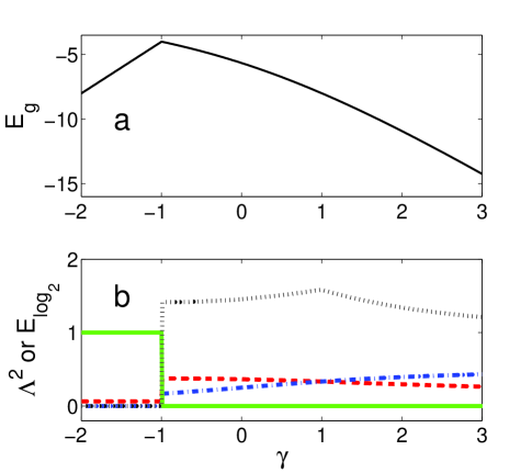
where $\alpha\in(-\pi/2,0)$ is given via $\tan(2\alpha)=-2\sqrt{2}/\gamma$, and $|\phi_{1}\rangle\equiv(|0101\rangle+|1010\rangle)/\sqrt{2}$, $|\phi_{2}\rangle\equiv(|1100\rangle+|0011\rangle+|1001\rangle+|0110\rangle)/2$. Fig. 1 (a) shows $E_{g}$ as a function of $\gamma$. One should note that $E_{g}$ is continuous at $\gamma=-1$ while the ground state $|g\rangle$ is discontinuous.

In order to obtain the ground-state GE, one needs to search for the closest product state $|\Psi^{*}\rangle$  OrusWei . In fact, we can choose the product states

$$|\Psi^{*}(\gamma)\rangle=\begin{cases}\,\,|\Psi_{1}\rangle\equiv|1111\rangle&(\gamma<-1)\\ \,\,|\Psi_{2}\rangle\equiv|+-+-\rangle&(-1<\gamma<1)\\ \,\,|\Psi_{3}\rangle\equiv|0101\rangle&(\gamma>1)\end{cases}$$ (4)

to obtain the corresponding entanglement in the respective range of $\gamma$. To anticipate the experimental procedure, we shall measure the ground-state overlap listed as

$$\Lambda_{1}(\gamma)=\langle\Psi_{1}|g\rangle=\begin{cases}1&(\gamma<-1)\\ 0&(\gamma>-1)\end{cases}$$ (5)

$$\Lambda_{2}(\gamma)=\langle\Psi_{2}|g\rangle=\begin{cases}\frac{1}{4}&(\gamma<-1)\\ \frac{\sqrt{2}}{4}\cos\alpha-\frac{1}{2}\sin\alpha&(\gamma>-1)\end{cases}$$ (6)

$$\Lambda_{3}(\gamma)=\langle\Psi_{3}|g\rangle=\begin{cases}0&(\gamma<-1)\\ \frac{1}{\sqrt{2}}\cos\alpha&(\gamma>-1)\end{cases}.$$ (7)

From Eqs. (6) and (7), one finds that $\Lambda_{2}(\gamma)$ and $\Lambda_{3}(\gamma)$ cross at $\gamma=1$. Fig. 1 (b) shows the theoretical prediction for $\Lambda^{2}_{i}(\gamma)$ ($i=1$, $2$, $3$) and the entanglement $E_{\log_{2}}$. The jump in the entanglement at $\gamma=-1$ and the cusp at $\gamma=1$ signify the two QPT points.

Figure 2: (Color online). Experimentally measured $\Lambda^{2}_{i}(\gamma)$ (a) and $E_{\log_{2}}$ (b) for various $\gamma$. In figure (a), the experimental data are shown as ”$\cdot$”, ”$\times$” and ”*” for $\Lambda^{2}_{i}=|\langle\Psi_{i}|g\rangle|^{2}$, corresponding to $|\Psi_{1}\rangle$, $|\Psi_{2}\rangle$ and $|\Psi_{3}\rangle$. The measured $\Lambda^{2}_{i}(\gamma)$ for $\gamma<-1$ are indicated as the dotted, dashed and dash-dotted lines. In the region $\gamma>-1$, $\Lambda^{2}_{1}(\gamma)$ can be fitted as the dotted line. Through fitting the points for $\Lambda^{2}_{2}(\gamma)$ and $\Lambda^{2}_{3}(\gamma)$ using polynomial functions, we obtain the two solid curves that cross at point $\gamma=0.92$, close to the theoretical point at $\gamma=1$. The thick dashed and dash-dotted curves show the fitting results using the theoretical $\Lambda^{2}_{2}(\gamma)$ and $\Lambda^{2}_{3}(\gamma)$ by introducing decay factors $0.69$ and $0.71$, respectively. In figure (b), in range $\gamma<-1$, $E_{\log_{2}}$ is shown as ”+”. For $\gamma>-1$, we rescale the measured $\Lambda^{2}_{2}(\gamma)$ and $\Lambda^{2}_{3}(\gamma)$ as $\Lambda^{2}_{2}(\gamma)/0.69$ and $\Lambda^{2}_{3}(\gamma)/0.71$, respectively. The dotted and dashed curves that cross at $\gamma=1.02$ show the fitting results of the rescaled data using polynomial functions. The expected $E_{\log_{2}}$ after rescaling is indicated by ”$\circ$”.

Figure 3: (Color online). Theoretical (a) and experimentally measured (b) $\Lambda^{2}$ for various product states created as $U_{p}(\beta)|0101\rangle$ [see Eq. (8)] . Three ground states for $\gamma=-0.9$, $1$ and $3$ are chosen and the corresponding $\Lambda^{2}$ are shown as the the solid, dash-dotted and dashed curves in figure (a), respectively. The experimental data are shown as ”*”, ”$\cdot$” and ”$\times$” for $\gamma=-0.9$, $1$ and $3$ in figure (b), respectively. In comparison with the theoretical values, they can be fitted as $0.66\Lambda^{2}$, $0.68\Lambda^{2}$ and $0.71\Lambda^{2}$, shown as the solid, dash-dotted and dashed curves.

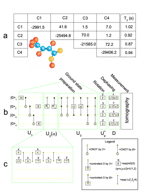
In experiment, we choose the four carbons in crotonic acid crot dissolved in d6-acetone as the four qubits. We generate the ground states using quantum networks and implement the quantum gates by GRAPE pulses GRAPE . Various ground-states can be created by varying the single spin rotations that can be easily implemented (see Supplemental Material). In principle, one can employ an iterative method to experimentally measure the GE of the ground state (see Supplemental Material). To demonstrate the proof-of-principle simulation of quantum entanglement, instead, we first measure the overlap of the ground state with several product states (4), which contain the closest product states. From the measurement with the already known closest product states, we can obtain the ground-state GE. Next, to show that the obtained results are the optimum, we vary the product states to test the optimality.

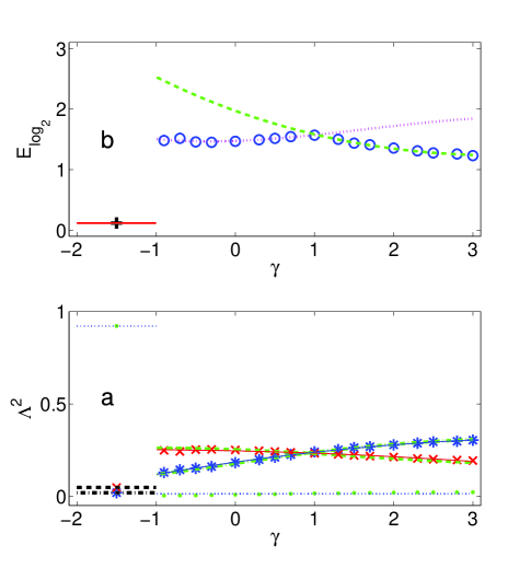
The experimentally measured $\Lambda_{i}^{2}(\gamma)$ for various $\gamma$ are shown in Fig. 2 (a). The measured $\Lambda^{2}_{i}(\gamma)$ for $\gamma<-1$ are $0.92$, $0.048$ and $0.019$, indicated as the dotted, dashed and dash-dotted lines. The corresponding theoretical values are $1$, $1/16$ and $0$, respectively. In the region $\gamma>-1$, $\Lambda^{2}_{1}(\gamma)$ can be fitted as $\Lambda^{2}_{1}(\gamma)=0.014$, shown as the dotted line, corresponding to $0$ in theory.

We perform polynomial fits to the measured $\Lambda^{2}_{2}(\gamma)$ and $\Lambda^{2}_{3}(\gamma)$, and obtain the two solid curves that cross at the point $\gamma=0.92$, which is very close to the theoretically predicted transition point at $\gamma=1$. The discrepancy between experiment and theory mainly comes from the different experimental errors in measuring $\Lambda^{2}_{2}(\gamma)$ and $\Lambda^{2}_{3}(\gamma)$. The jump at $\gamma=-1$ and the cusp at $\gamma=0.92$ reflect the different types of QPT points.

In order to faithfully estimate the performance of the experiment in measuring $\Lambda^{2}_{2}(\gamma)$ and $\Lambda^{2}_{3}(\gamma)$ in the range $\gamma>-1$, we introduce two decay factors $\alpha_{2}$ and $\alpha_{3}$ to fit the experimental data as $[\Lambda^{2}_{2,3}(\gamma)]_{{\rm exp}}=\alpha_{2,3}[\Lambda^{2}_{2,3}(\gamma)]_{{\rm theory}}$, shown as the thick dashed and dash-dotted curves in Fig. 2 (a) with the best scale-factors as $\alpha_{2}=0.69$ and $\alpha_{3}=0.71$, respectively. The difference between the decay factors comes from the different operations in measuring $\Lambda^{2}_{2}(\gamma)$ and $\Lambda^{2}_{3}(\gamma)$. In Fig. 2 (b), we exploit the decay factors to rescale experimental values of $[\Lambda^{2}_{2,3}]_{\rm exp}/\alpha_{2,3}$, from which we obtain the expected values of pseudo-entanglement shown as ”$\circ$”. The rescaled $-\log_{2}([\Lambda^{2}_{2,3}]_{\rm exp}/\alpha_{2,3})$ can be fitted as the dotted and dashed curves that cross at $\gamma=1.02$.

In principle, we do not need to know the closest product states in order to measure the entanglement. In the Supplemental Material, we describe an iterative procedure to search for them and this procedure can be implemented in experiment. For proof-of-principle demonstration of the optimality experimentally, we simplify the procedure and vary the product states $|\Psi(\beta)\rangle$ by

$$|\Psi(\beta)\rangle=U_{p}(\beta)|0101\rangle,$$ (8)

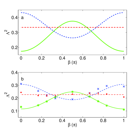
where $U_{p}(\beta)=\bigotimes_{j=1}^{4}e^{-i\beta Y_{j}/2}$, and experimentally measure $\Lambda^{2}=|\langle\Psi(\beta)|g\rangle|{{}^{2}}$ for various $\beta$ at three different locations of the phase diagram, corresponding to $\gamma=-0.9$, $1$, and $3$, respectively. The theoretical and experimental results are shown in Figs. 3(a) and (b), respectively. The experimental data are compared to the theoretical values of $0.66\Lambda^{2}$, $0.68\Lambda^{2}$ and $0.71\Lambda^{2}$, shown in Fig. 3 (b). One finds that the maximum of $\Lambda^{2}$ occurs at $\beta=\pi/2$ and $0$ for $\gamma=-0.9$ and $3$, respectively. These correspond to the respective closest product states, $|\Psi_{2}\rangle=|+-+-\rangle$ and $|\Psi_{3}\rangle=|0101\rangle$, predicted theoretically. Remarkably, for $\gamma=1$, where the $\infty$-order QPT occurs, $\Lambda^{2}$ is a constant independent of $\beta$, as we have expected and noted earlier. This also means that arbitrary states prepared by Eq. (8) can be chosen to measure the entanglement at $\gamma=1$, and this gives additional confirmation that the created state at the KT point is rotationally invariant.

The experiment duration of the preparation of the ground states for $\gamma>-1$ is about 160 ms, which is non-negligible (about 17%) compared to the coherence time $T_{2}$. Consequently the decay of the signals due to the limitation of coherence time is one of main sources of errors. Additionally the imperfection of pulses and inhomogeneities of magnetic fields also contribute to errors. The deviations of the experimental data from the theoretical fitting in Fig. 3 (b) represent the effects of the errors that depend on the rotation angles, or the product states. In particular the fluctuation of the data for $\gamma=1$ in Fig. 3 (b) confirms the explanation for the shift of the measured cusp in Fig. 2 (a).

In conclusion we demonstrate the non-analytic properties of many-body systems in a quantum simulator using NMR. The QPTs with first- and $\infty$-orders in the XXZ spin chain are detected by directly measuring the pseudo-entanglement of the ground states created by quantum gates. An alternative approach for creating ground states would be via adiabatic evolution Peng09 . Our preliminary numerical analysis indicates that ground states for $\gamma>-1$ can be approximately generated with high fidelity (e.g. $>0.998$) by the adiabatic evolution from the ground state at a large $\gamma$. The experimental implementation is a possible future direction.

We thank O. Moussa and R. Orús for helpful discussions. This work was supported by CIFAR (R.L.), NSERC (J.-F.Z., R.L. and T.-C.W.), MITACS (T.-C.W.), SHARCNET (R.L.), and QuantumWorks (R.L.).

Supplemental Material

Appendix A Method for computing and measuring the maximal overlap by iteration

Here we describe an iterative method to compute the maximal overlap, of which the motivation comes from the density-matrix-renormalization-group (DMRG) or matrix-product-state (MPS) variational method mps . This method can not only be implemented numerically, but can also be carried out experimentally. To compute the maximal overlap for the state $|g\rangle$ with respect to product states $|\Psi\rangle\equiv\bigotimes_{i=1}^{N}|\psi^{(i)}\rangle$, we use the Lagrange multiplier $\lambda$ to enforce the constraint $\langle\Psi|\Psi\rangle=1$,

$$f(\Psi)\equiv\langle\Psi|g\rangle\langle g|\Psi\rangle-\lambda\langle\Psi|\Psi\rangle.$$ (9)

Maximizing $f$ with respect to the local product state $|\psi^{(i)}\rangle$, we obtain the extremal condition

$${\cal H}_{\rm eff}^{(i)}|\psi^{(i)}\rangle=\lambda N^{(i)}|\psi^{(i)}\rangle,$$ (10)

where ${\cal H}_{\rm eff}^{(i)}\equiv(\bigotimes_{j\neq i}^{N}\langle\psi^{(j)}|)|g\rangle\langle g|(\bigotimes_{j\neq i}^{N}|\psi^{(j)}\rangle)$ is proportional to a local projector (labeled by $|\phi^{(i)}\rangle\langle\phi^{(i)}|$ at $i$-site), and the normalization $N^{(i)}\equiv\bigotimes_{j\neq i}^{N}\langle\psi^{(j)}|\psi^{(j)}\rangle$, is unity if all the local states are properly normalized. From the viewpoint of the variational MPS, one fixes all local states $|\psi^{(j)}\rangle$ but $|\psi^{(i)}\rangle$ and solves for the corresponding optimal $|\psi^{(i)}\rangle$ and repeats the same procedure for $i+1$, $i+2$, etc. until the $N$-th site and sweeps the procedure back and forth until the eigenvalue $\lambda$ converges. The converged value $|\lambda|^{2}$ is the square of the maximal overlap $\Lambda_{\max}^{2}$.

Experimentally, this procedure means that one chooses randomly the local measurement basis and picks arbitrarily one direction (i.e., rank-one projector) for each site, say, $|\psi^{(j)}\rangle$ for the $j$-th site and only varies the basis for one site, say, $i$-th at a time with all others fixed until one reaches a basis where the measurement outcome along one direction occurs with the most probability. Then one moves to the next site, say, $(i+1)$-th site, and finds the optimal direction and repeats this procedure by sweeping back and forth until the probability for the most likely outcome converges.

Numerically, it appears that one has to solve the above eigenvalue problem. But as the effective local Hamiltonian is a projector, one immediately sees that the optimal rank-one projector is exactly the one ($|\phi^{(i)}\rangle\langle\phi^{(i)}|$) given by ${\cal H}_{\rm eff}^{(i)}$. One thus replaces $|\psi^{(i)}\rangle$ by $|\phi^{(i)}\rangle$ and repeats the procedure at other sites until the overlap converges. Experimentally, the apparatus setting in line with the projector gives the local maximum output probability. The search for the optimal direction at the $i$-th site need not be a blind search, as a tomography (conditioned on all other sites being measured in their respective $|\psi^{(j)}\rangle$) will enable the determination of the optimal local direction $|\phi^{(i)}\rangle$. The whole procedure, either numerically or experimentally, thus becomes an iterative procedure, given an initial choice of $\{|\psi^{(j)}\rangle\}$. We have performed such a numerical procedure and have found that this procedure converges efficiently to the maximal overlap. The convergence for the ground state of four-spin chain is very fast and the result is accurate; see Fig. 4. In our experiment, we implement a simplified version to directly measure the ground-state entanglement.

Figure 4: (Color online). Numerical implementation of the iteration procedure for the maximal overlap in the 4-spin XXZ chain. The overlap square is shown as marked as ”*”, ”$\cdot$” and ”$\times$” for $\gamma=-0.9$, $1$ and $3$, respectively. An initial 4-spin product state is randomly chosen. One round of sweep starts from the first spin, reaches the forth spin, and sweeps back to the second spin. One round thus contains six steps. Eight iteration rounds are shown. The maximal overlap squares converge rapidly to their exact values, which are indicated by the thin lines, after just a few rounds. We have checked that the converged product states are $|+-+-\rangle$ (up to a relative phase), $|\phi\phi^{\perp}\phi\phi^{\perp}\rangle$ (with $\langle\phi^{\perp}|\phi\rangle=0$), and $|0101\rangle$, respectively.

Appendix B Method for solving the 4-spin XXZ chain

For $\gamma<-1$ the ground state is doubly degenerate with ground states being $|0000\rangle$ and $|1111\rangle$. To avoid the complication due to the degeneracy, we can introduce an additional small Zeeman term $H_{z}=B_{z}\sum_{i=1}^{N}Z_{i}$ with $0<B_{z}\ll 1$ into the Hamiltonian to lift the energy of $|0000\rangle$ so that the ground state $|g\rangle$ becomes $|1111\rangle$. The small Zeeman term does not affect the universality class of phase transition of the ground state, because it commutes with $H_{XXZ}$.

For $\gamma>-1$, the ground state is not a simple product state. Due to the absence of an external field, the conservation of z-component total angular momentum and the periodic translation invariance give rise to only two relevant “Bethe-ansatz” basis states for the ground states:

$$|\phi_{1}\rangle \equiv \frac{1}{\sqrt{2}}(|0101\rangle+|1010\rangle)$$ (11)

$$|\phi_{2}\rangle \equiv \frac{1}{2}(|1100\rangle+|0011\rangle+|1001\rangle+|0110\rangle).$$ (12)

By solving the effective Hamiltonian in the subspace spanned by $\{|\phi_{1}\rangle,|\phi_{2}\rangle\}$

$$H_{eff}=-4\left(\begin{array}[]{cc}\gamma&-\sqrt{2}\\ -\sqrt{2}&0\\ \end{array}\right)$$ (13)

we obtain that the ground state is

$$|g\rangle=|\phi_{1}\rangle\cos\alpha+|\phi_{2}\rangle\sin\alpha$$ (14)

where $\alpha\in(-\pi/2,0)$ is given via

$$\tan(2\alpha)=-2\sqrt{2}/\gamma,$$ (15)

and that the ground energy is

$$E_{g}(\gamma)=-2\gamma-2\sqrt{\gamma^{2}+8}.$$ (16)

Appendix C Method for experimental implementation

The experiment is performed in a Bruker DRX 700 MHz spectrometer. The structure of the molecule of crotonic acid and the parameters of the four spin qubits are shown in Fig. 5 (a). The protons are decoupled in the whole experiment. The initial pseudo-pure state $|0000\rangle$ is prepared by spatial averaging zhang09a ; pures , and chosen as the reference state for normalizing the signals in the following partial state tomography.

The quantum circuit shown as Fig. 5 (b) illustrates the experiment protocol for $\gamma>-1$. The ground state is created by $U_{3}U_{2}(\alpha)U_{1}$, indicated by the three dashed blocks, respectively. We optimize $U_{1}$ and $U_{3}$, which are independent of $\alpha$, as two long (40 ms duration) GRAPE pulses, respectively, where GRAPE stands for gradient ascent pulse engineering. The theoretical fidelity for $U_{1}$ and $U_{3}$ is larger than $99\%$. To save time in searching GRAPE pulses, we further decompose $U_{2}(\alpha)$ into simple gates shown as the sequence in Fig. 5 (c), where each gate is implemented by one GRAPE pulse. The duration of the pulse for the spin coupling evolution is 20 ms, and the duration of other pulses is 0.5 ms. The theoretical fidelity for each pulse in Fig. 5 (c) is larger than $99.5\%$. An arbitrary ground state for $\gamma>-1$ can be generated through varying $\alpha$ in the single spin operation, which is much easier to find than $U_{2}(\alpha)$ in the GRAPE algorithm. For the case of $\gamma<-1$, we replace $U_{3}U_{2}(\alpha)U_{1}$ by four NOT gates implemented by four $\pi$ pulses applied to the four qubits respectively to create the ground state $|1111\rangle$ from $|0000\rangle$.

To measure the overlap between $|g\rangle$ and an arbitrary product state $|\Psi\rangle$, we re-write the overlap $\Lambda\equiv\langle\Psi|g\rangle$ in form of

$$\Lambda=\langle b|U^{{\dagger}}_{p}|g\rangle$$ (17)

where $|b\rangle$ denotes a computational basis and $U_{p}|b\rangle=|\Psi\rangle$ zhang09a . Here we choose $U_{p}$ as

$$U_{p}(\beta)=\bigotimes_{j=1}^{4}e^{-i\beta Y_{j}/2}.$$ (18)

Since $|\Psi_{1}\rangle$ and $|\Psi_{3}\rangle$ are already the computational basis, we can simply choose $|b\rangle$ as $|\Psi_{1}\rangle$ and $|\Psi_{3}\rangle$, respectively, and take $U_{p}$ as the identity operation by setting $\beta=0$, for obtaining $\Lambda_{1}$ and $\Lambda_{3}$ from Eq. (17). $|\Psi_{2}\rangle$ is not a computational basis. We can choose $|b\rangle=|0101\rangle$ and $\beta=\pi/2$ for obtaining $\Lambda_{2}$, noting that $|\Psi_{2}\rangle=U_{p}(\pi/2)|0101\rangle$.

In the density-matrix form, Eq. (17) is represented as

$$\Lambda^{2}=Tr(|b\rangle\langle b|\rho)$$ (19)

where $\rho=U_{p}^{{\dagger}}(|g\rangle\langle g|)U_{p}$. From Eq. (19), one finds that $\Lambda^{2}$ is encoded as the diagonal element $|b\rangle\langle b|$ of $\rho$. We exploit phase cycling to remove all the non-diagonal elements, and then reconstruct all the diagonal terms of $\rho$ using partial state tomographgy through four $\pi/2$ readout pulses selective for C1-C4, respectively. $\Lambda^{2}$ is therefore extracted from the diagonal terms.

Figure 5: (Color online). Experimental protocol. (a) The molecule structure (inset) and the parameters of the four carbon-13 spins. The diagonal terms show the chemical shifts and the non-diagonal terms show the strength of $J$- couplings in Hz. The transversal relaxation times $T_{2}$ measured by a Hahn echo are listed in the rightmost column. (b) Quantum circuit for creating the ground state and measuring its overlap $\Lambda_{i}(\gamma)$ for $\gamma>-1$. Here $\mathbf{X}$ denotes a NOT gate. $R_{\pm\alpha}=\exp{(\pm i\alpha Y)}$, and $\mathbf{H}$ ( $\mathbf{H^{*}}$) denotes a gate transforming state $|0\rangle$ ($|1\rangle$) to $(|0\rangle$ + $|1\rangle)/\sqrt{2}$, and $|1\rangle$ ($|0\rangle$) to $(|0\rangle$ - $|1\rangle)/\sqrt{2}$, respectively. The other gates are illustrated in the legend box. $U_{2}$ is decomposed as the gate sequence shown in (c), for creating an arbitrary ground state for $\gamma>-1$ through varying $\alpha$ [see Eq. (15)]. $U_{p}$ denotes a rotation for obtaining the overlap of the ground-state with $U_{p}|b\rangle$, where $|b\rangle$ denotes a computational basis. In dephasing operation, $j$, $k$, $m$, $n$ are chosen as $0$ and $1$, respectively, to average out all non-diagonal terms in the density matrix to zero. Tomograhpy of the diagonal terms requires four $\pi/2$ pulses selective for C1 to C4, respectively.

References

- (1) A. Einstein, B. Podolsky, and N. Rosen, Phys. Rev. 47, 777 (1935).
- (2) M. Nielsen and I. Chuang, Quantum Computation and Quantum Information (Cambridge University Press, Cambridge, 2000).
- (3) R. Horodecki et al., Rev. Mod. Phys. 81, 865 (2009).
- (4) S. Sachdev, Quantum Phase Transitions (Cambridge University Press, Cambridge, England, 2000).
- (5) A. Osterloh et al., Nature (London) 416, 608 (2002).
- (6) S. Sachdev, Nature Phys. 4, 173 (2008).
- (7) L. Amico et al., Rev. Mod. Phys. 80, 517 (2008).
- (8) O. Gühne and G. Tóth, Physics Reports 474, 1 (2009).
- (9) P. Horodecki, Phys. Rev. Lett. 90, 167901 (2003); H. A. Carteret, ibid. 94, 040502 (2005).
- (10) S. P. Walborn et al., Nature 440, 1022 (2006); N. Kiesel et al., Phys. Rev. Lett. 101, 260505 (2008).
- (11) O. Gühne, M. Reimpell and R.F. Werner, Phys. Rev. Lett. 98, 110502 (2007).
- (12) R. P. Feynman, Int. J. Theor. Phys. 21, 467 (1982); S. Lloyd, Science 273, 1073 (1996); I. Buluta and F. Nori, ibid. 326, 108 (2009).
- (13) V. E. Korepin et al., Quantum Inverse Scattering Method and Correlation Functions (Cambridge University Press, Cambridge 1997).
- (14) L. M. K. Vandersypen and I. L. Chuang, Rev. Mod. Phys. 76, 1037 (2004); J. A. Jones, Prog. in NMR Spectrosc. 38, 325 (2001).
- (15) T.-C. Wei and P. M. Goldbart, Phys. Rev. A 68, 042307 (2003).
- (16) T.-C. Wei et al., Phys. Rev. A 71, 060305(R) (2005).
- (17) J. M. Kosterlitz and D. J. Thouless, J. of Phys. C 6, 1181-1203 (1973).
- (18) C. C. Rulli and M. S. Sarandy, Phys. Rev. A 81, 032334 (2010).
- (19) L.-A. Wu et al., Phys. Rev. Lett. 93, 250404 (2004); S.-J. Gu, Int. J. Mod. Phys. B 24, 4371(2010).
- (20) R. Orús and T.-C. Wei, Phys. Rev. B. 82, 155120 (2010).
- (21) R. Orús, Phys. Rev. Lett. 100, 130502 (2008); R. Orús et al., ibid. 101, 025701 (2008).
- (22) M. Hayashi et al., Phys. Rev. Lett. 96, 040501 (2006).
- (23) D. Gross et al., Phys. Rev. Lett. 102, 190501 (2009).
- (24) Here is equivalent to or more generally with due to the symmetry in the ground states. Similarly, is equivalent to .
- (25) E. Knill et al., Nature (London) 404, 368 (2000).
- (26) N. Khaneja et al., J. Magn. Reson. 172, 296 (2005); C. A. Ryan et al., Phys. Rev. A 78, 012328 (2008).
- (27) P. Krl, I. Thanopulos and M. Shapiro, Rev. Mod. Phys. 79, 53 (2007); X. Peng et al., Phys. Rev. Lett. 103, 140501 (2009).
- (1) F. Verstraete et al., Adv. Phys. 57, 143 (2008).
- (2) J. S. Hodges et al., Phys. Rev. A 75, 042320 (2007).
- (3) J. Zhang et al., Phys. Rev. A 79, 012305 (2009).