Linear Dependent Types and Relative Completeness*

Abstract.

A system of linear dependent types for the $\lambda$-calculus with full higher-order recursion, called $\mathsf{d}\ell\mathsf{PCF}$, is introduced and proved sound and relatively complete. Completeness holds in a strong sense: $\mathsf{d}\ell\mathsf{PCF}$ is not only able to precisely capture the functional behavior of $\mathsf{PCF}$ programs (i.e. how the output relates to the input) but also some of their intensional properties, namely the complexity of evaluating them with Krivine’s Machine. $\mathsf{d}\ell\mathsf{PCF}$ is designed around dependent types and linear logic and is parametrized on the underlying language of index terms, which can be tuned so as to sacrifice completeness for tractability.

1. Introduction

Type systems are powerful tools in the design of programming languages. While they have been employed traditionally to guarantee weak properties of programs (e.g. “well-typed programs cannot go wrong”), it is becoming more and more evident that they can be useful when stronger properties are needed, such as security [33, 32], termination [6], monadic temporal properties [26] or resource bounds [25, 11].

One key advantage of type systems seen as formal methods is their simplicity and their close relationship with programs — checking whether a program has a type or even inferring the (most general) type of a program is often decidable. The price to pay is the incompleteness of most type systems: there are programs satisfying the property at hand which cannot be given a type. This is in contrast with other formal methods, like program logics [2] where completeness is always a desirable feature, although it only holds relatively to an oracle. Graphically, the situation is similar to the one in Figure 1: type systems are bound to be in the lower left corner of the diagram, where both the degree of completeness and the complexity of the property under consideration is low; program logics, on the other hand, are confined to the upper-right corner, where checking for derivability is almost always undecidable.

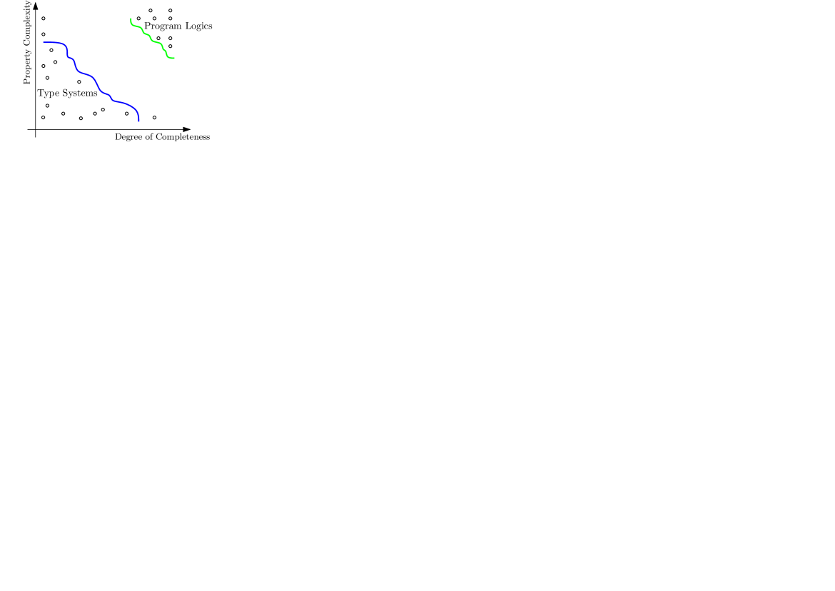
Figure 1. Type Systems and Program Logics

One specific research field in which the just-described scenario manifests itself is implicit computational complexity, in which one aims at defining characterizations of complexity classes by programming languages and logical systems. Many type systems have been introduced capturing, for instance, the polynomial time computable functions [23, 5, 4]. All of them, under mild assumptions, can be employed as tools to certify programs as asymptotically time efficient. However, a tiny slice of the polytime programs are generally typable, since the underlying complexity class $\mathbf{FP}$ is only characterized in a purely extensional sense — for every function in $\mathbf{FP}$ there is at least one typable program computing it.

The main contribution of this paper is a type system for the $\lambda$-calculus with full recursion, called $\mathsf{d}\ell\mathsf{PCF}$, which is sound and complete. Types of $\mathsf{d}\ell\mathsf{PCF}$ are obtained, in the spirit of $\mathsf{DML}$ [36, 35], by decorating types of ordinary $\mathsf{PCF}$ [31, 21] with index terms. These are first-order terms freely generated from variables, function symbols and a few more term constructs. They are indicated with metavariables like $\mathrm{I},\mathrm{J},\mathrm{K}$. Type decoration reflects the standard decomposition of types into linear types (as suggested by linear logic [18]), and is inspired by recent works on the expressivity of bounded logics [13].

Index terms and linear types permit to describe program properties with a fine granularity. More precisely, $\mathsf{d}\ell\mathsf{PCF}$ enjoys the following two properties:

• Soundness: if $t$ is a program and $\vdash_{\mathrm{K}}t:{\tt Nat}[\mathrm{I},\mathrm{J}]$, then $t$ evaluates to a natural number which lies between $\mathrm{I}$ and $\mathrm{J}$ and this evaluation takes at most $(\mathrm{K}+1)\cdot|t|$ steps;

• Completeness: if $t$ is typable in $\mathsf{PCF}$ and evaluates to a natural number $n$ in $m$ steps, then $\vdash_{\mathrm{I}}t:{\tt Nat}[\textbf{n},\textbf{n}]$, where $\mathrm{I}\leq m$.

Completeness of $\mathsf{d}\ell\mathsf{PCF}$ holds not only for programs (i.e. terms of ground types) but also for functions on the natural numbers (see Section 5.3 for further details). Moreover, typing judgments tell us something about the functional behavior of programs but also about their non-functional one, namely the number of steps needed to evaluate the term in Krivine’s Abstract Machine.

As the title of this paper suggests, completeness of $\mathsf{d}\ell\mathsf{PCF}$ holds in a relative sense. Indeed, the behavior of programs can be precisely captured only in presence of a complete oracle for the truth of certain assumptions in typing rules. This is exactly what happens in program logics such as Floyd-Hoare’s logic, where all true partial correctness assertions can be derived provided one is allowed to use all true sentences of first order arithmetic as axioms [10]. In $\mathsf{d}\ell\mathsf{PCF}$, those assumptions take the form of (in)equalities between index terms, to be verified when function symbols are interpreted as partial functions on natural numbers according to an equational program $\mathcal{E}$. Actually, the whole of $\mathsf{d}\ell\mathsf{PCF}$ is parametrized on such an $\mathcal{E}$, but while soundness holds independently of the specific $\mathcal{E}$, completeness, as is to be expected, holds only if $\mathcal{E}$ is sufficiently powerful to encode all total computable functions (i.e. if $\mathcal{E}$ is universal). In other words, $\mathsf{d}\ell\mathsf{PCF}$ can be claimed to be not a type system, but a family of type systems obtained by taking a specific $\mathcal{E}$ as the underlying “logic” of index terms. The simpler $\mathcal{E}$, the easier type checking and type inference are; the more complex $\mathcal{E}$, the larger the class of captured programs.

The design of $\mathsf{d}\ell\mathsf{PCF}$ has been very much influenced by linear logic [18], and in particular by systems of indexed and bounded linear logic [19, 13], which have been recently shown to subsume other ICC systems as for the class of programs they capture [13]. One of the many ways to “read” $\mathsf{d}\ell\mathsf{PCF}$ is as a variation on the theme of $\mathsf{BLL}$ [19] obtained by generalizing polynomials to arbitrary functions. The idea of going beyond a restricted, fixed class of bounds comes from Xi’s work on $\mathsf{DML}$ [36, 35]. Cost recurrences for first order $\mathsf{DML}$ programs have been studied [20]. No similar completeness results for dependent types are known, however.

2. Types and Program Properties: An Informal Account

Consider the following program:

$$\mathtt{dbl}={\tt fix}\ f.\lambda x.{\ \tt ifz\ }x{\ \tt then\ }\underline{\tt 0}{\ \tt else\ }{\tt s}({\tt s}(f({\tt p}(x)))).$$

In a monomorphic, traditionally designed type system like $\mathsf{PCF}$ [31, 21], the term $\mathtt{dbl}$ receives type ${\tt Nat}\rightarrow{\tt Nat}$. As a consequence, $\mathtt{dbl}$ computes a function on natural numbers without “going wrong”: it takes in input a natural number, and produces in output another natural number (if any). The type ${\tt Nat}\rightarrow{\tt Nat}$, however, does not give any information about which specific function on the natural numbers $\mathtt{dbl}$ computes. Indeed, in $\mathsf{PCF}$ (and in most real-world programming languages) any program computing a function on natural numbers, being it for instance the identity function or (a unary version of) the Ackermann function, can be typed by ${\tt Nat}\rightarrow{\tt Nat}$.

Some modern type systems allow one to construct and use types like $\tau={\tt Nat}[a]\rightarrow{\tt Nat}[\textbf{2}\times a]$, which tell not only what set or domain (the interpretation of) the term belongs to, but also which specific element of the domain the term actually denotes. The type $\tau$, for example, could be attributed only to those programs computing the function $n\mapsto 2\times n$, including $\mathtt{dbl}$. Types of this form can be constructed in dependent and sized type theories [36, 6]. The type system $\mathsf{d}\ell\mathsf{PCF}$ introduced in this paper offers this possibility, too. But, as a first contribution, it further allows to specify imprecise types, like ${\tt Nat}[\textbf{5},\textbf{8}]$, which stands for the type of those natural numbers between $5$ and $8$ (included).

A property of programs which is completely ignored by ordinary type systems is termination, at least if full recursion is in the underlying language. Typing a term $t$ with ${\tt Nat}\rightarrow{\tt Nat}$ does not guarantee that $t$, when applied to a natural number, terminates. In $\mathsf{PCF}$ this is even worse: $t$ could possibly diverge itself! Consider, as another example, a slight modification of $\mathtt{dbl}$, namely

$$\mathtt{omega}={\tt fix}\ f.\lambda x.{\ \tt ifz\ }x{\ \tt then\ }\underline{\tt 0}{\ \tt else\ }{\tt s}({\tt s}(f(x))).$$

It behaves as $\mathtt{dbl}$ when fed with $0$, but it diverges when it receives a positive natural number as an argument. But look: $\mathtt{omega}$ is not so different from $\mathtt{dbl}$. Indeed, the second can be obtained from the first by feeding not $x$ but ${\tt p}(x)$ to $f$. And any type systems in which $\mathtt{dbl}$ and $\mathtt{omega}$ are somehow recognized as being fundamentally different must be able to detect the presence of ${\tt p}$ in $\mathtt{dbl}$ and deduct termination from it. Indeed, sized types [6] and dependent types [34] are able to do so.

Going further, we could ask the type system to be able not only to guarantee termination, but also to somehow evaluate the time or space consumption of programs. For example, we could be interested in knowing that $\mathtt{dbl}$ takes a polynomial number of steps to be evaluated on any natural number. This cannot be achieved neither using classical type systems nor using systems of sized types, at least when traditionally formulated. However, some type systems able to control the complexity of programs exist. Good examples are type systems for amortized analysis [25, 22] or those using ideas from linear logic [5, 4]. In those type systems, typing judgements carry, besides the usual type information, some additional information about the resource consumption of the underlying program. As an example, $\mathtt{dbl}$ could be given a type as follows

$$\vdash_{\mathrm{I}}\mathtt{dbl}:{\tt Nat}\to{\tt Nat}$$

where $\mathrm{I}$ is some cost information for $\mathtt{dbl}$. This way, building a type derivation and inferring resource consumption can be done at the same time.

The type system $\mathsf{d}\ell\mathsf{PCF}$ we propose in this paper makes some further steps in this direction. First of all, it combines some of the ideas presented above with the ones of bounded linear logic. $\mathsf{BLL}$ allows one to explicitly count the number of times functions use their arguments (in rough notation, $!_{\textbf{m}}\sigma\multimap\tau$ says that the argument of type $\sigma$ is used $m$ times). This permits to extract natural cost functions from type derivations. The cost of evaluating a term will be measured by counting how many times function arguments need to be copied during evaluation. Making this information explicit in types permits to compute the cost step by step during the type derivation process. By the way, previous works by the first author [12] show that this way of attributing a cost to (proofs seen as) programs is sound and precise as a way to measure their time complexity. Intuitively, typing judgements in $\mathsf{d}\ell\mathsf{PCF}$ can be thought as:

$$\vdash_{\mathrm{J}}t\ :\ !_{\textbf{m}}\ {\tt Nat}[a]\multimap{\tt Nat}[\mathrm{I}].$$

where $\mathrm{I}$ and $\mathrm{J}$ can be derived while building a type derivation, exploiting the information carried by the modalities. In fact, the quantitative information in $!_{\textbf{m}}$ allows to statically determine the number of times any subterm will be copied during evaluation. But this is not sufficient: analogously to what happens in $\mathsf{BLL}$, $\mathsf{d}\ell\mathsf{PCF}$ makes types more parametric. A rough type as $!_{\textbf{n}}\sigma\multimap\tau$ is replaced by the more parametric type $[{a<\textbf{n}}]\cdot{\sigma}\multimap\tau$, which tells us that the argument will be used $n$ times, and each instance has type $\sigma$ where, however the variable $a$ is instantiated with a value less than $n$. This allows to type each copy of the argument differently but uniformly, since all instances of $\sigma$ have the same $\mathsf{PCF}$ skeleton. This form of uniform linear dependence is actually crucial in obtaining the result which makes $\mathsf{d}\ell\mathsf{PCF}$ different from similar type systems, namely completeness.

Finally, as already stressed in the Introduction, $\mathsf{d}\ell\mathsf{PCF}$ is also parametric in the class of functions (in the form of an equational program $\mathcal{E}$) that can be used to reason about types and costs. This permits to tune the type system, as described in Section 6 below.

Anticipating on the next section, we can say that $\mathtt{dbl}$ can be typed as follows in $\mathsf{d}\ell\mathsf{PCF}$:

$$\vdash_{a}^{\mathcal{E}}\mathtt{dbl}:[{b<a+\textbf{1}}]\cdot{{\tt Nat}}[a]\multimap{\tt Nat}[\textbf{2}\times a].$$

This tells us that the argument will be used $a+1$ times by $\mathtt{dbl}$, and that the cost of evaluation will be itself proportional to $a$.

3. $\mathsf{d}\ell\mathsf{PCF}$

In this section, the language of programs and the type system $\mathsf{d}\ell\mathsf{PCF}$ for it will be introduced formally. Some of their basic properties will be described. The type system $\mathsf{d}\ell\mathsf{PCF}$ is based on the notion of an index term whose semantics, in turn, is defined by an equational program. As a consequence, all these notions must be properly introduced and are the subject of Section 3.1 below.

3.1. Index Terms and Equational Programs

Syntactically, index terms are built either from function symbols from a given signature or by applying any of two special term constructs.

Formally, a signature $\Sigma$ is a pair $(\mathcal{S},\alpha)$ where $\mathcal{S}$ is a finite set of function symbols and $\alpha:\mathcal{S}\rightarrow\mathbb{N}$ assigns an arity to every function symbol. Index terms on a given signature $\Sigma=(\mathcal{S},\alpha)$ are generated by the following grammar:

$$\mathrm{I},\mathrm{J},\mathrm{K} ::=a\;\;\mbox{\Large{$\mid$}}\;\;\texttt{f}(\mathrm{I}_{1},\ldots,\mathrm{I}_{\alpha(\texttt{f})})\;\;\mbox{\Large{$\mid$}}\;\;\displaystyle{\sum_{a<\mathrm{I}}\mathrm{J}}\;\;\mbox{\Large{$\mid$}}\;\;\displaystyle{\bigotriangleup_{a}^{\mathrm{I},\mathrm{J}}\mathrm{K}},$$

where $\texttt{f}\in\mathcal{S}$ and $a$ is a variable drawn from a set $\mathcal{V}$ of index variables. We assume the symbols 0, 1 (with arity $0$) and $+$, $\dotdiv$ (with arity $2$) are always part of $\Sigma$. An index term in the form $\sum_{a<\mathrm{I}}\mathrm{J}$ is a bounded sum, while one in the form $\bigotriangleup_{a}^{\mathrm{I},\mathrm{J}}\mathrm{K}$ is a forest cardinality. For every natural number $n$, the index term n is just

$$\underbrace{\textbf{1}+\textbf{1}+\ldots+\textbf{1}}_{\mbox{$n$ times}}.$$

Index terms are meant to denote natural numbers, possibly depending on the (unknown) values of variables. Variables can be instantiated with other index terms, e.g. $\mathrm{I}\{\mathrm{J}/a\}$. So, index terms can also act as first order functions. What is the meaning of the function symbols from $\Sigma$? It is the one induced by an equational program $\mathcal{E}$. Formally, an equational program $\mathcal{E}$ over a signature $\Sigma$ and a set of variables $\mathcal{V}$ is a set of equations in the form $t=s$ where both $t$ and $s$ are terms in the free algebra $\mathcal{O}(\Sigma,\mathcal{V})$ over $\Sigma$ and $\mathcal{V}$. We are interested in equational programs guaranteeing that, whenever symbols in $\Sigma$ are interpreted as partial functions over $\mathbb{N}$ and 0, 1, $+$ and $\dotdiv$ are interpreted in the usual way, the semantics of any function symbol f can be uniquely determined from $\mathcal{E}$. This can be guaranteed by, for example, taking $\mathcal{E}$ as an Herbrand-Gödel scheme [30] or as an orthogonal constructor term rewriting system [3]. One may wonder why the definition of index terms is parametric on $\Sigma$ and $\mathcal{E}$. As we will see in Section 6, being parametric this way allows us to tune our concrete type system from a highly undecidable but truly powerful machinery down to a tractable but less expressive formal system. An example of an equational program over the signature $\Sigma$ consisting of three function symbols gt, add and mult of arity two is the following sequence of equations:

$$\texttt{gt}(\textbf{0},b) =\textbf{0};$$

$$\texttt{gt}(a+\textbf{1},\textbf{0}) =\textbf{1};$$

$$\texttt{gt}(a+\textbf{1},b+\textbf{1}) =\texttt{gt}(a,b);$$

$$\texttt{add}(\textbf{0},b) =b;$$

$$\texttt{add}(a+\textbf{1},b) =\texttt{add}(a,b)+\textbf{1};$$

$$\texttt{mult}(\textbf{0},b) =\textbf{0};$$

$$\texttt{mult}(a+\textbf{1},b) =\texttt{add}(b,\texttt{mult}(a,b)).$$

What about the meaning of bounded sums and forest cardinalities? The first is very intuitive: the value of $\sum_{a<\mathrm{I}}\mathrm{J}$ is simply the sum of all possible values of $\mathrm{J}$ with $a$ taking the values from $0$ up to $\mathrm{I}$, excluded. Forest cardinalities, on the other hand, require some more effort to be described. Informally, $\bigotriangleup_{a}^{\mathrm{I},\mathrm{J}}\mathrm{K}$ is an index term denoting the number of nodes in a forest composed of $\mathrm{J}$ trees described using $\mathrm{K}$. All the nodes in the forest are (uniquely) identified by natural numbers. These are obtained by consecutively visiting each tree in pre-order, starting from $\mathrm{I}$. The term $\mathrm{K}$ has the role of describing the number of children of each forest node $n$ by properly instantiating the variable $a$, e.g the number of children of the root (of the leftmost tree in the forest) is $\mathrm{K}\{\textbf{0}/a\}$. More formally, the meaning of a forest cardinality is defined by the following two equations:

$$\bigotriangleup_{a}^{\mathrm{I},\textbf{0}}\mathrm{K} =\textbf{0};$$ (1)

$$\bigotriangleup_{a}^{\mathrm{I},\mathrm{J}+\textbf{1}}\mathrm{K} =\left(\bigotriangleup_{a}^{\mathrm{I},\mathrm{J}}\mathrm{K}\right)+\textbf{1}+\left(\bigotriangleup_{a}^{\mathrm{I}+\textbf{1}+\bigotriangleup_{a}^{\mathrm{I},\mathrm{J}}\mathrm{K},\mathrm{K}\{\mathrm{I}+\bigotriangleup_{a}^{\mathrm{I},\mathrm{J}}\mathrm{K}/a\}}\mathrm{K}\right).$$ (2)

Equation (1) says that a forest of $0$ trees contains no nodes. Equation (2) tells us that a forest of $\mathrm{J}+1$ trees contains:

• the nodes in the first $\mathrm{J}$ trees;

• and the nodes in the last tree, which are just one plus the nodes in the immediate subtrees of the root, considered themselves as a forest.

To better understand forest cardinalities, consider the following forest comprising two trees:

and consider an index term $\mathrm{K}$ with a free index variable $a$ such that $\mathrm{K}\{\textbf{n}/a\}=3$ for $n=1$; $\mathrm{K}\{\textbf{n}/a\}=2$ for $n\in\{2,8\}$; $\mathrm{K}\{\textbf{n}/a\}=1$ when $n\in\{0,6,9,11\}$; and $\mathrm{K}\{\textbf{n}/a\}=0$ when $n\in\{3,4,7,10,12\}$. That is, $\mathrm{K}$ describes the number of children of each node in the forest. Then $\bigotriangleup_{a}^{\textbf{0},\textbf{2}}\mathrm{K}=\textbf{13}$ since it takes into account the entire forest; $\bigotriangleup_{a}^{\textbf{0},\textbf{1}}\mathrm{K}=\textbf{8}$ since it takes into account only the leftmost tree; $\bigotriangleup_{a}^{\textbf{8},\textbf{1}}\mathrm{K}=\textbf{5}$ since it takes into account only the second tree of the forest; finally, $\bigotriangleup_{a}^{\textbf{2},\textbf{3}}\mathrm{K}=\textbf{6}$ since it takes into account only the three trees (as a forest) in the dashed rectangle.

One may wonder what is the role of forest cardinalities in the type system. Actually, they play a crucial role in the treatment of recursive calls, where the unfolding of recursion produces a tree-like structure whose size is just the number of times the (recursively defined) function will be used globally. Note that the value of a forest cardinality could also be undefined. For instance, this happens when infinite trees, corresponding to diverging recursive computations, are considered.

The expression $\llbracket\mathrm{I}\rrbracket^{\mathcal{E}}_{\rho}$ denotes the meaning of $\mathrm{I}$, defined by induction along the lines of the previous discussion, where $\rho:\mathcal{V}\rightarrow\mathbb{N}$ is an assignment and $\mathcal{E}$ is an equational program giving meaning to the function symbols in $\mathrm{I}$. Since $\mathcal{E}$ does not necessarily interpret such symbols as total functions, and moreover, the value of a forest cardinality can be undefined, $\llbracket\mathrm{I}\rrbracket^{\mathcal{E}}_{\rho}$ can be undefined itself. A constraint is an inequality in the form $\mathrm{I}\leq\mathrm{J}$. A constraint is true in an assignment $\rho$ if $\llbracket\mathrm{I}\rrbracket^{\mathcal{E}}_{\rho}$ and $\llbracket\mathrm{J}\rrbracket^{\mathcal{E}}_{\rho}$ are both defined and the first is smaller or equal to the latter. Now, for a subset $\phi$ of $\mathcal{V}$, and for a set $\Phi$ of constraints involving variables in $\phi$, the expression

$$\phi;\Phi\models^{\mathcal{E}}\mathrm{I}\leq\mathrm{J}$$ (3)

denotes the fact that the truth of $\mathrm{I}\leq\mathrm{J}$ semantically follows from the truth of the constraints in $\Phi$. The expression $\phi;\Phi\models^{\mathcal{E}}\mathrm{I}\geq\textbf{0}$ indicates that (the semantics of) $\mathrm{I}$ is defined for the relevant values of the variables in $\phi$; this is usually written as $\phi;\Phi\models^{\mathcal{E}}\mathrm{I}\Downarrow$.

Similarly, one can define the meaning of expressions like $\phi;\Phi\models^{\mathcal{E}}\mathrm{I}=\mathrm{J}$ or $\phi;\Phi\models^{\mathcal{E}}\mathrm{I}\simeq\mathrm{J}$, the latter standing for the equality of $\mathrm{I}$ and $\mathrm{J}$ in the sense of Kleene, i.e. $\phi;\Phi\models^{\mathcal{E}}\mathrm{I}\Downarrow$ if and only if $\phi;\Phi\models^{\mathcal{E}}\mathrm{J}\Downarrow$, and if $\phi;\Phi\models^{\mathcal{E}}\mathrm{I}\Downarrow$ then $\phi;\Phi\models^{\mathcal{E}}\mathrm{I}=\mathrm{J}$. When both $\phi$ and $\Phi$ are empty, such expressions can be written in a much more concise form, e.g. $\mathrm{I}\simeq\mathrm{J}$ stands for $\emptyset;\emptyset\models^{\mathcal{E}}\mathrm{I}\simeq\mathrm{J}$.

The following two lemmas about forest cardinalities are useful, and will be crucial when proving the Substitution Lemma.

Lemma 1.

For every index terms $\mathrm{I},\mathrm{J},\mathrm{K},\mathrm{H}$, we have:

$$\bigotriangleup_{a}^{\mathrm{I}+\mathrm{J},\mathrm{K}}\mathrm{H}\simeq\bigotriangleup_{a}^{\mathrm{J},\mathrm{K}}\mathrm{H}\{a+\mathrm{I}/a\}.$$

Proof 3.1.

The proof is by coinduction on the definition of $\bigotriangleup_{a}^{\mathrm{I}+\mathrm{J},\mathrm{K}}\mathrm{H}$ by distinguishing the cases for the different values of $\mathrm{K}$. For $\mathrm{K}\simeq\textbf{0}$ we have both:

$$\bigotriangleup_{a}^{\mathrm{I}+\mathrm{J},\textbf{0}}\mathrm{H}\simeq\textbf{0};\qquad\bigotriangleup_{a}^{\mathrm{J},\textbf{0}}\mathrm{H}\{a+\mathrm{I}/a\}\simeq\textbf{0}.$$

For $\mathrm{K}\simeq\mathrm{L}+\textbf{1}$ we have:

$$\bigotriangleup_{a}^{\mathrm{I}+\mathrm{J},\mathrm{L}+\textbf{1}}\mathrm{H}\simeq\bigotriangleup_{a}^{\mathrm{I}+\mathrm{J},\mathrm{L}}\mathrm{H}+\textbf{1}+\bigotriangleup_{a}^{\mathrm{I}+\mathrm{J}+\textbf{1}+\bigotriangleup_{a}^{\mathrm{I}+\mathrm{J},\mathrm{L}}\mathrm{H},\mathrm{H}\{\mathrm{I}+\mathrm{J}+\bigotriangleup_{a}^{\mathrm{I}+\mathrm{J},\mathrm{L}}\mathrm{H}/a\}}\mathrm{H},$$

and analogously

$$\bigotriangleup_{a}^{\mathrm{J},\mathrm{L}+\textbf{1}}\mathrm{H}\{a+\mathrm{I}/a\}\simeq\bigotriangleup_{a}^{\mathrm{J},\mathrm{L}}\mathrm{H}\{a+\mathrm{I}/a\}+\textbf{1}+\bigotriangleup_{a}^{\mathrm{J}+1+\bigotriangleup_{a}^{\mathrm{J},\mathrm{L}}\mathrm{H}\{a+\mathrm{I}/a\},\mathrm{H}\{\mathrm{I}+\mathrm{J}+\bigotriangleup_{a}^{\mathrm{J},\mathrm{L}}\mathrm{H}\{a+\mathrm{I}/a\}/a\}}\mathrm{H}\{a+\mathrm{I}/a\}.$$

This concludes the proof.

Lemma 2.

For every index term of the shape $\bigotriangleup_{a}^{\textbf{1},\mathrm{J}}\mathrm{I}$ we have:

$$\bigotriangleup_{a}^{\textbf{1},\mathrm{J}}\mathrm{I}\simeq\sum_{b<\mathrm{J}}\bigotriangleup_{a}^{\textbf{0},\textbf{1}}\mathrm{I}\{a+\textbf{1}+\bigotriangleup_{a}^{\textbf{1},b}\mathrm{I}/a\}.$$

Proof 3.2.

The proof is by coinduction on the definition of $\bigotriangleup_{a}^{\textbf{1},\mathrm{J}}\mathrm{I}$ by distinguishing the cases for the different values of $\mathrm{J}$. For $\mathrm{J}\simeq\textbf{0}$, we have both:

$$\bigotriangleup_{a}^{\textbf{1},\textbf{0}}\mathrm{I}\simeq\textbf{0};\qquad\sum_{b<\textbf{0}}\bigotriangleup_{a}^{\textbf{0},\textbf{1}}\mathrm{I}\{a+\textbf{1}+\bigotriangleup_{a}^{\textbf{1},b}\mathrm{I}/a\}\simeq\textbf{0}.$$

For $\mathrm{J}\simeq\mathrm{L}+\textbf{1}$ we have

$$\bigotriangleup_{a}^{\textbf{1},\mathrm{L}+\textbf{1}}\mathrm{I}\simeq\mathrm{K}+\textbf{1}+\bigotriangleup_{a}^{\mathrm{K}+\textbf{2},\mathrm{I}\{\mathrm{K}+\textbf{1}/a\}}\mathrm{I}$$

and

$$\sum_{b<\mathrm{L}+\textbf{1}}\bigotriangleup_{a}^{\textbf{0},\textbf{1}}\mathrm{I}\{a+\textbf{1}+\bigotriangleup_{a}^{\textbf{1},b}\mathrm{I}/a\}\simeq\mathrm{H}+\bigotriangleup_{a}^{\textbf{0},\textbf{1}}\mathrm{I}\{a+\textbf{1}+\bigotriangleup_{a}^{\textbf{1},\mathrm{L}}\mathrm{I}/a\},$$

where $\mathrm{K}$ is $\bigotriangleup_{a}^{\textbf{1},\mathrm{L}}\mathrm{I}$ and $\mathrm{H}$ is $\sum_{b<\mathrm{L}}\bigotriangleup_{a}^{\textbf{0},\textbf{1}}\mathrm{I}\{a+\textbf{1}+\bigotriangleup_{a}^{\textbf{1},b}\mathrm{I}/a\}$. Now, by definition and by Lemma 1, we have

$$\bigotriangleup_{a}^{\textbf{0},\textbf{1}}\mathrm{I}\{a+\textbf{1}+\bigotriangleup_{a}^{\textbf{1},\mathrm{L}}\mathrm{I}/a\}\simeq\textbf{1}+\bigotriangleup_{a}^{\textbf{1},\mathrm{I}\{\mathrm{K}+\textbf{1}/a\}}\mathrm{I}\{a+\textbf{1}+\mathrm{K}/a\}\simeq\textbf{1}+\bigotriangleup_{a}^{\mathrm{K}+\textbf{2},\mathrm{I}\{\mathrm{K}+\textbf{1}/a\}}\mathrm{I}.$$

This concludes the proof.

Before embarking in the description of the type system, a further remark on the role of index terms could be useful. Index terms are not meant to be part of programs but of types. As a consequence, computation will not be carried out on index terms but on proper terms, which are the subject of Section 3.2 below.

3.2. The Type System

Terms are generated by the following grammar:

$$t::= x\;\;\mbox{\Large{$\mid$}}\;\;\underline{\tt n}\;\;\mbox{\Large{$\mid$}}\;\;{\tt s}(t)\;\;\mbox{\Large{$\mid$}}\;\;{\tt p}(t)\;\;\mbox{\Large{$\mid$}}\;\;\lambda x.t\;\;\mbox{\Large{$\mid$}}\;\;tu$$

$$\;\;\mbox{\Large{$\mid$}}\;\;{\ \tt ifz\ }t{\ \tt then\ }u{\ \tt else\ }v\;\;\mbox{\Large{$\mid$}}\;\;{\tt fix}\ x.t$$

where $\tt n$ ranges over natural numbers and $x$ ranges over a set of variables. As usual, terms which are equal modulo $\alpha$-conversion are considered equal. This, in turn, allows to define the notion of substitution in the standard way. The set of head subterms of any term $t$ can be defined easily by induction on the structure of $t$, e.g. the head subterms of $t=uv$ are $t$ itself and the head subterms of $u$ (but not those of $v$).

A notion of size $|t|$ for a term $t$ will be useful in the sequel. This can be defined as follows:

$$|x| =1; |\lambda x.t| =|t|+1;$$

$$|\underline{\tt n}| =1; |tu| =|t|+|u|+1;$$

$$|{\tt s}(t)| =|t|+2; |{\ \tt ifz\ }t{\ \tt then\ }u{\ \tt else\ }v| =|t|+|u|+|v|+1;$$

$$|{\tt p}(t)| =|t|+2; |{\tt fix}\ x.t| =|t|+1.$$

Notice that for technical reasons size is defined in a slightly nonstandard way: every integer constant has size $1$.

Lemma 3.

If $t$ is a term and $u$ is a subterm of $t$, then $|u|\leq|t|$.

Terms can be typed by a well-known type system called $\mathsf{PCF}$. Types are those generated by the basic type ${\tt Nat}$ and the binary type constructor $\rightarrow$. Typing rules are in Figure 2.

$$\begin{array}[]{ccccc}\Gamma,x:\sigma\vdash x:\sigma&&\Gamma\vdash\lambda x.t:\sigma\rightarrow\tau\Gamma,x:\sigma\vdash t:\tau&&\Gamma\vdash tu:\tau\lx@proof@logical@and\Gamma\vdash t:\sigma\rightarrow\tau\Gamma\vdash u:\sigma\end{array}$$ $$\begin{array}[]{ccccc}\Gamma\vdash\underline{\tt n}:{\tt Nat}&&\Gamma\vdash{\tt s}(t):{\tt Nat}\Gamma\vdash t:{\tt Nat}&&\Gamma\vdash{\tt p}(t):{\tt Nat}\Gamma\vdash t:{\tt Nat}\end{array}$$ $$\begin{array}[]{ccc}\Gamma\vdash{\ \tt ifz\ }t{\ \tt then\ }u{\ \tt else\ }v:\sigma\lx@proof@logical@and\Gamma\vdash t:{\tt Nat}\Gamma\vdash u:\sigma\Gamma\vdash v:\sigma&&\Gamma\vdash{\tt fix}\ x.t:\sigma\Gamma,x:\sigma\vdash t:\sigma\end{array}$$

Figure 2. The $\mathsf{PCF}$ Type System.

A notion of weak-head reduction $\to$ can be easily defined: see Figure 3.

$$\begin{array}[]{ccccccc}(\lambda x.t)u\to t\{u/x\}&&{\tt s}(\underline{\tt n})\to\underline{\tt n+1}&&{\tt p}(\underline{\tt n+1})\to\underline{\tt n}&&{\tt p}(\underline{\tt 0})\to\underline{\tt 0}\end{array}$$ $$\begin{array}[]{ccccc}{\ \tt ifz\ }\underline{\tt 0}{\ \tt then\ }u{\ \tt else\ }v\to u&&{\ \tt ifz\ }\underline{\tt n+1}{\ \tt then\ }u{\ \tt else\ }v\to v\end{array}$$ $$\begin{array}[]{ccccccc}{\tt fix}\ x.t\to t\{{\tt fix}\ x.t/x\}&&{\tt s}(t)\to{\tt s}(u)t\to u&&{\tt p}(t)\to{\tt p}(u)t\to u&&tu\to vut\to v\end{array}$$ $${\ \tt ifz\ }t{\ \tt then\ }u{\ \tt else\ }v\to{\ \tt ifz\ }w{\ \tt then\ }u{\ \tt else\ }vt\to w$$

Figure 3. Weak-head Reduction

A term $t$ is said to be a program if it can be given the $\mathsf{PCF}$ type ${\tt Nat}$ in the empty context.

Almost all the definitions about $\mathsf{d}\ell\mathsf{PCF}$ in this and the next sections should be understood as parametric on an equational program $\mathcal{E}$ over a signature $\Sigma$. For the sake of simplicity, however, we will often avoid to explicitly mention $\mathcal{E}$ and leave it implicit.

$\mathsf{d}\ell\mathsf{PCF}$ can be seen as a refinement of $\mathsf{PCF}$ obtained by a linear decoration of its type derivations. Basic and modal types are defined as follows:

$$\sigma,\tau ::={\tt Nat}[\mathrm{I},\mathrm{J}]\;\;\mbox{\Large{$\mid$}}\;\;A\multimap\sigma;$$ basic types

$$A,B ::=[{a<\mathrm{I}}]\cdot{\sigma};$$ modal types

where $\mathrm{I},\mathrm{J}$ range over index terms and $a$ ranges over index variables. ${\tt Nat}[\mathrm{I}]$ is syntactic sugar for ${\tt Nat}[\mathrm{I},\mathrm{I}]$. Modal types need some comments. As a first approximation, they can be thought of as quantifiers over type variables. So, a type like $A=[{a<\mathrm{I}}]\cdot{\sigma}$ acts as a binder for the index variable $a$ in the basic type $\sigma$. Moreover, the condition $a<\mathrm{I}$ says that $A$ consists of all the instances of the basic type $\sigma$ where the variable $a$ is successively instantiated with the values from 0 to (the value of) $\mathrm{I}\dotdiv\textbf{1}$, i.e. $\sigma\{\textbf{0}/a\},\ldots,\sigma\{\mathrm{I}\dotdiv\textbf{1}/a\}$ . For those readers who are familiar with linear logic, and in particular with $\mathsf{BLL}$, the modal type $[{a<\mathrm{I}}]\cdot{\sigma}$ is a generalization of the $\mathsf{BLL}$ formula $!_{a<p}\sigma$ to arbitrary index terms. As such it can be thought of as representing the type $\sigma\{\textbf{0}/a\}\otimes\cdots\otimes\sigma\{\mathrm{I}\dotdiv\textbf{1}/a\}$. In analogy to what happens in the standard linear logic decomposition of the intuitionistic arrow, i.e. $!A\multimap B=A\Rightarrow B$, it is sufficient to restrict to modal types appearing in negative position.Finally, for those readers with some knowledge of $\mathsf{DML}$, modal types are in a way similar to $\mathsf{DML}$’s subset sort constructions [35].

We always assume that index terms appearing inside types are defined for all the relevant values of the variables in $\phi$. This is captured by the judgement $\phi;\Phi\vdash^{\mathcal{E}}\sigma\Downarrow$, whose rules are in Figure 4.

$$\begin{array}[]{ccc}\phi;\Phi\vdash^{\mathcal{E}}{\tt Nat}[\mathrm{I},\mathrm{J}]\Downarrow\begin{array}[]{c}\phi;\Phi\models^{\mathcal{E}}\mathrm{I}\Downarrow\\ \phi;\Phi\models^{\mathcal{E}}\mathrm{J}\Downarrow\\ \end{array}&&\phi;\Phi\vdash^{\mathcal{E}}A\multimap\sigma\Downarrow\begin{array}[]{c}\phi;\Phi\vdash^{\mathcal{E}}A\Downarrow\\ \phi;\Phi\vdash^{\mathcal{E}}\sigma\Downarrow\end{array}\end{array}$$ $$\phi;\Phi\vdash^{\mathcal{E}}[{a<\mathrm{I}}]\cdot{\sigma}\Downarrow\begin{array}[]{c}\phi,a;\Phi,a<\mathrm{I}\vdash^{\mathcal{E}}\sigma\Downarrow\\ \phi;\Phi\models^{\mathcal{E}}\mathrm{I}\Downarrow\\ \end{array}$$

Figure 4. Well-defined Types

In the typing rules, modal types need to be manipulated in an algebraic way. For this reason, two operations on modal types need to be introduced. The first one is a binary operation $\uplus$ on modal types. Suppose that $A=[{a<\mathrm{I}}]\cdot{\mu\{a/c\}}$ and that $B=[{b<\mathrm{J}}]\cdot{\mu\{\mathrm{I}+b/c\}}$. In other words, $A$ consists of the first $\mathrm{I}$ instances of $\mu$, i.e. $\mu\{\textbf{0}/c\},\ldots,\mu\{\mathrm{I}\dotdiv\textbf{1}/c\}$ while $B$ consists of the next $\mathrm{J}$ instances of $\mu$, i.e. $\mu\{\mathrm{I}+\textbf{0}/c\},\ldots,\mu\{\mathrm{I}+\mathrm{J}\dotdiv\textbf{1}/c\}$. Their sum $A\uplus B$ is naturally defined as a modal type consisting of the first $\mathrm{I}+\mathrm{J}$ instances of $\mu$, i.e. $[{c<\mathrm{I}+\mathrm{J}}]\cdot{\mu}$. An operation of bounded sum on modal types can be defined by generalizing the idea above. Suppose that $A=[{b<\mathrm{J}}]\cdot{\sigma\{\sum_{d<a}\mathrm{J}\{d/a\}+b/c\}}$. Then its bounded sum $\sum_{a<\mathrm{I}}A$ is $[{c<\sum_{a<\mathrm{I}}\mathrm{J}}]\cdot{\sigma}$.

To every type $\sigma$ corresponds a type $(\!|\sigma|\!)$ of ordinary $\mathsf{PCF}$, namely a type built from the basic type ${\tt Nat}$ and the arrow operator $\rightarrow$:

$$(\!|{\tt Nat}[\mathrm{I},\mathrm{J}]|\!) ={\tt Nat};$$

$$(\!|[{a<\mathrm{I}}]\cdot{\sigma}\multimap\tau|\!) =(\!|\sigma|\!)\rightarrow(\!|\tau|\!).$$

Central to $\mathsf{d}\ell\mathsf{PCF}$ is the notion of subtyping. An inequality relation $\sqsubseteq$ between (basic and modal) types can be defined by way of the formal system in Figure 5. This relation corresponds to lifting index inequalities at the type level.

$$\begin{array}[]{ccccc}\phi;\Phi\vdash^{\mathcal{E}}{\tt Nat}[\mathrm{I},\mathrm{J}]\sqsubseteq{\tt Nat}[\mathrm{K},\mathrm{H}]\begin{array}[]{c}\phi;\Phi\models^{\mathcal{E}}\mathrm{K}\leq\mathrm{I}\\ \phi;\Phi\models^{\mathcal{E}}\mathrm{J}\leq\mathrm{H}\\ \end{array}&&\phi;\Phi\vdash^{\mathcal{E}}A\multimap\sigma\sqsubseteq B\multimap\tau\begin{array}[]{c}\phi;\Phi\vdash^{\mathcal{E}}B\sqsubseteq A\\ \phi;\Phi\vdash^{\mathcal{E}}\sigma\sqsubseteq\tau\end{array}&\end{array}$$ $$\phi;\Phi\vdash^{\mathcal{E}}[{a<\mathrm{I}}]\cdot{\sigma}\sqsubseteq[{a<\mathrm{J}}]\cdot{\tau}\begin{array}[]{c}\phi,a;\Phi,a<\mathrm{I}\vdash^{\mathcal{E}}\sigma\sqsubseteq\tau\\ \phi;\Phi\models^{\mathcal{E}}\mathrm{J}\leq\mathrm{I}\\ \end{array}$$

Figure 5. The Subtyping Relation

The equivalence $\phi;\Phi\vdash\sigma\cong\tau$ holds when both $\phi;\Phi\vdash\sigma\sqsubseteq\tau$ and $\phi;\Phi\vdash\tau\sqsubseteq\sigma$ can be derived from the rules in Figure 5. $\phi;\Phi\vdash\sigma\Downarrow$ is syntactic sugar for $\phi;\Phi\vdash\sigma\sqsubseteq\sigma$.

It is now time to introduce the main object of this paper, namely the type system $\mathsf{d}\ell\mathsf{PCF}$. Typing judgements of $\mathsf{d}\ell\mathsf{PCF}$ are expressions in the form

$$\phi;\Phi;\Gamma\vdash_{\mathrm{I}}^{\mathcal{E}}t:\sigma,$$ (4)

where $\Gamma$ is a typing context, that is, a set of term variable assignments of the shape $x:A$ where each variable $x$ occurs at most once. The expression (4) can be informally read as follows: for every values of the index variables in $\phi$ satisfying $\Phi$, $t$ can be given type $\sigma$ and cost $\mathrm{I}$ once its free term variables have types as in $\Gamma$. In proving this, equations from $\mathcal{E}$ can play a role.

Typing rules are in Figure 6, where binary and bounded sums are used in their natural generalization to contexts. A type derivation is nothing more than a tree built according to typing rules. A precise type derivation is a type derivation such that all premises in the form $\sigma\sqsubseteq\tau$ (respectively, in the form $\mathrm{I}\leq\mathrm{J}$) are required to be in the form $\sigma\cong\tau$ (respectively, $\mathrm{I}=\mathrm{J}$).

$$\begin{array}[]{ccc}\phi;\Phi;\Gamma,x:[{a<\mathrm{I}}]\cdot{\sigma}\vdash_{\mathrm{J}}^{\mathcal{E}}x:\tau\begin{array}[]{c}\phi;\Phi\models^{\mathcal{E}}\textbf{0}\leq\mathrm{J}\qquad\phi;\Phi\models^{\mathcal{E}}\textbf{1}\leq\mathrm{I}\\ \phi;\Phi\vdash^{\mathcal{E}}\sigma\{\textbf{0}/a\}\sqsubseteq{\tau}\\ \phi;\Phi\vdash^{\mathcal{E}}([{a<\mathrm{I}}]\cdot{\sigma})\Downarrow\qquad\phi;\Phi\vdash^{\mathcal{E}}\Gamma\Downarrow\end{array}&&\phi;\Phi;\Gamma\vdash^{\mathcal{E}}_{\mathrm{J}}\lambda x.t:[{a<\mathrm{I}}]\cdot{\sigma}\multimap\tau\phi;\Phi;\Gamma,x:[{a<\mathrm{I}}]\cdot{\sigma}\vdash^{\mathcal{E}}_{\mathrm{J}}t:\tau\end{array}$$ $$\begin{array}[]{ccc}\phi;\Phi;\Sigma\vdash^{\mathcal{E}}_{\mathrm{H}}tu:\tau\begin{array}[]{c}\phi;\Phi;\Gamma\vdash^{\mathcal{E}}_{\mathrm{J}}t:[{a<\mathrm{I}}]\cdot{\sigma}\multimap\tau\\ \phi,a;\Phi,a<\mathrm{I};\Delta\vdash^{\mathcal{E}}_{\mathrm{K}}u:\sigma\\ \phi;\Phi\vdash^{\mathcal{E}}\Sigma\sqsubseteq\Gamma\uplus\sum_{a<\mathrm{I}}{\Delta}\\ \phi;\Phi\models^{\mathcal{E}}\mathrm{H}\geq\mathrm{J}+\mathrm{I}+{\sum_{a<\mathrm{I}}\mathrm{K}}\end{array}&&\phi;\Phi;\Gamma\vdash^{\mathcal{E}}_{\mathrm{L}}{\tt s}(t):{\tt Nat}[\mathrm{K},\mathrm{H}]\begin{array}[]{c}\phi;\Phi\vdash^{\mathcal{E}}{\tt Nat}[\mathrm{I}+\textbf{1},\mathrm{J}+\textbf{1}]\sqsubseteq{\tt Nat}[\mathrm{K},\mathrm{H}]\\ \phi;\Phi;\Gamma\vdash^{\mathcal{E}}_{\mathrm{L}}t:{\tt Nat}[\mathrm{I},\mathrm{J}]\end{array}\end{array}$$ $$\begin{array}[]{ccc}\phi;\Phi;\Gamma\vdash^{\mathcal{E}}_{\mathrm{K}}\underline{\tt n}:{\tt Nat}[\mathrm{I},\mathrm{J}]\begin{array}[]{c}\phi;\Phi\models^{\mathcal{E}}\mathrm{K}\geq\textbf{0}\\ \phi;\Phi\models^{\mathcal{E}}\mathrm{I}\leq\textbf{n}\\ \phi;\Phi\models^{\mathcal{E}}\textbf{n}\leq\mathrm{J}\\ \phi;\Phi\vdash^{\mathcal{E}}\Gamma\Downarrow\end{array}&&\phi;\Phi;\Gamma\vdash^{\mathcal{E}}_{\mathrm{L}}{\tt p}(t):{\tt Nat}[\mathrm{K},\mathrm{H}]\begin{array}[]{c}\phi;\Phi\vdash^{\mathcal{E}}{\tt Nat}[\mathrm{I}\dotdiv\textbf{1},\mathrm{J}\dotdiv\textbf{1}]\sqsubseteq{\tt Nat}[\mathrm{K},\mathrm{H}]\\ \phi;\Phi;\Gamma\vdash^{\mathcal{E}}_{\mathrm{L}}t:{\tt Nat}[\mathrm{I},\mathrm{J}]\end{array}\end{array}$$ $$\phi;\Phi;\Sigma\vdash^{\mathcal{E}}_{\mathrm{L}}{\ \tt ifz\ }t{\ \tt then\ }u{\ \tt else\ }v:\sigma\begin{array}[]{c}\phi;\Phi;\Gamma\vdash^{\mathcal{E}}_{\mathrm{K}}t:{\tt Nat}[\mathrm{I},\mathrm{J}]\\ \phi;\Phi,\mathrm{I}\leq{\tt 0};\Delta\vdash^{\mathcal{E}}_{\mathrm{H}}u:\sigma\\ \phi;\Phi,\mathrm{J}\geq\textbf{1};\Delta\vdash^{\mathcal{E}}_{\mathrm{H}}v:\sigma\\ \phi;\Phi\vdash^{\mathcal{E}}\Sigma\sqsubseteq\Gamma\uplus\Delta\\ \phi;\Phi\models^{\mathcal{E}}\mathrm{L}\geq\mathrm{K}+\mathrm{H}\end{array}$$ $$\phi;\Phi;\Sigma\vdash^{\mathcal{E}}_{\mathrm{N}}{\tt fix}\ x.t:\mu\begin{array}[]{c}\phi,b;\Phi,b<\mathrm{L};\Gamma,x:[{a<\mathrm{I}}]\cdot{\sigma}\vdash^{\mathcal{E}}_{\mathrm{K}}t:\tau\\ \phi;\Phi\vdash^{\mathcal{E}}\tau\{\textbf{0}/b\}\sqsubseteq\mu\\ \phi,a,b;\Phi,a<\mathrm{I},b<\mathrm{L}\vdash^{\mathcal{E}}\tau\{\bigotriangleup_{b}^{b+\textbf{1},a}\mathrm{I}+b+\textbf{1}/b\}\sqsubseteq\sigma\\ \phi;\Phi\vdash^{\mathcal{E}}\Sigma\sqsubseteq\sum_{b<\mathrm{L}}\Gamma\\ \phi;\Phi\models^{\mathcal{E}}\bigotriangleup_{b}^{\textbf{0},\textbf{1}}\mathrm{I}\leq\mathrm{L},\mathrm{M}\\ \phi;\Phi\models^{\mathcal{E}}\mathrm{N}\geq\mathrm{M}\dotdiv\textbf{1}+\sum_{b<\mathrm{L}}\mathrm{K}\end{array}$$

Figure 6. Typing Rules

First of all, observe that the typing rules are syntax-directed: given a term $t$, all type derivations for $t$ end with the same typing rule, namely the one corresponding to the last syntax rule used in building $t$. In particular, no explicit subtyping rule exists, but subtyping is applied to the context in every rule. A syntax-directed type system offers a key advantage: it allows one to prove the statements about type derivations by induction on the structure of terms. This greatly simplifies the proof of crucial properties like subject reduction.

Typing rules have premises of three different kinds:

• Of course, typing a term requires typing its immediate subterms, so typing judgements can be rule premises.

• As just mentioned, typing rules allow to subtype the context $\Gamma$, so subtyping judgements can be themselves rule premises.

• The application of typing rules (and also of subtyping rules, see Figure 5) sometimes depends on the truth of some inequalities between index terms in the model induced by $\mathcal{E}$.

As a consequence, typing rules can only be applied if some relations between index terms are consequences of the constraints in $\Phi$. These assumptions have a semantic nature, but could of course be verified by any sound formal system. Completeness (see Section 5), however, only holds if all true inequalities can be used as assumptions. As a consequence, type inference but also type (derivation) checking are bound to be problematic from a computational point of view. See Section 6 for a more thorough discussion on this issue.

As a last remark, note that each rule can be seen as a decoration of a rule of ordinary $\mathsf{PCF}$. More: for every $\mathsf{d}\ell\mathsf{PCF}$ type derivation $\pi$ of $\phi;\Phi;\Gamma\vdash_{\mathrm{I}}^{\mathcal{E}}t:\sigma$ there is a structurally identical derivation in $\mathsf{PCF}$ for the same term, i.e. a derivation $(\!|\pi|\!)\mathrel{\rhd}(\!|\Gamma|\!)\vdash t:(\!|\sigma|\!)$.

3.3. An Example

In this section, we will show how $\mathsf{d}\ell\mathsf{PCF}$ can give a sensible type to the example we talked about in the Introduction, namely

$$\mathtt{dbl}={\tt fix}\ f.\lambda x.{\ \tt ifz\ }x{\ \tt then\ }\underline{\tt 0}{\ \tt else\ }{\tt s}({\tt s}(f({\tt p}(x)))).$$

First, let us take a look at a subterm of $\mathtt{dbl}$, namely $t={\ \tt ifz\ }x{\ \tt then\ }\underline{\tt 0}{\ \tt else\ }{\tt s}({\tt s}(f({\tt p}(x))))$. In plain $\mathsf{PCF}$, $t$ receives the type ${\tt Nat}$ in an environment where $x$ has type ${\tt Nat}$ and $f$ has type ${\tt Nat}\rightarrow{\tt Nat}$. Presumably, a $\mathsf{d}\ell\mathsf{PCF}$ type for $t$ can be obtained by decorating in an appropriate way the type above. In other words, we are looking for a type derivation with conclusion:

$$\phi;\Phi;x:[{a<\mathrm{I}}]\cdot{{\tt Nat}[\mathrm{J}]},f:[{b<\mathrm{K}}]\cdot{([{c<\mathrm{H}}]\cdot{{\tt Nat}}[\mathrm{L}]\multimap{\tt Nat}[\mathrm{M}])}\vdash^{\mathcal{E}}_{\mathrm{N}}t:{\tt Nat}[\mathrm{P}].$$

But how should we proceed? What we would like, at the end of the day, is being able to describe how the value of $t$ depends on the value of $x$, so we could look for a type derivation in this form:

$$d;\emptyset;x:[{\mathrm{I}}]\cdot{{\tt Nat}[d]},f:[{b<\mathrm{K}}]\cdot{([{\mathrm{H}}]\cdot{{\tt Nat}}[d\dotdiv\textbf{1}]\multimap{\tt Nat}[\textbf{2}(d\dotdiv\textbf{1})])}\vdash^{\mathcal{E}}_{\mathrm{N}}t:{\tt Nat}[\textbf{2}d],$$

where $[{a<\mathrm{I}}]$ (respectively, $[{c<\mathrm{H}}]$) has been abbreviated into $[{\mathrm{I}}]$ (respectively, $[{\mathrm{H}}]$) because the bound variable $a$ (respectively, $c$) does not appear free in the underlying type. But how to give values to $\mathrm{I}$, $\mathrm{K}$, and $\mathrm{H}$? One could be tempted to define $\mathrm{I}$ simply as 2, since there are two occurrences of $x$ in $t$. However, in view of the role played by $x$ and $f$ in $\mathtt{dbl}$, $\mathrm{I}$ should be rather defined taking into account the number of times $x$ will be copied along the computation of $\mathtt{dbl}$ on any input. A good guess could be, for example, $d+\textbf{1}$. Similarly, $\mathrm{H}$ could be $d$. But how about $\mathrm{K}$? How many times $f$ is used? If $d=0$, then $f$ is not called, while if $d>\textbf{0}$, the function is called once. In other words, a guess for $\mathrm{H}$ could be $\texttt{gt}(d,\textbf{0})$. Here we use the infix notation $>$ for the operator gt just to improve readability. Let us now try to build a derivation for

$$d;\emptyset;x:[{d+\textbf{1}}]\cdot{{\tt Nat}[d]},f:[{d>\textbf{0}}]\cdot{([{d}]\cdot{{\tt Nat}}[d\dotdiv\textbf{1}]\multimap{\tt Nat}[\textbf{2}(d\dotdiv\textbf{1})])}\vdash^{\mathcal{E}}_{\textbf{0}}t:{\tt Nat}[\textbf{2}d].$$

Actually, it has the following shape:

$$d;\emptyset;x:[{d+\textbf{1}}]\cdot{{\tt Nat}[d]},f:[{d>\textbf{0}}]\cdot{([{d}]\cdot{{\tt Nat}}[d\dotdiv\textbf{1}]\multimap{\tt Nat}[\textbf{2}(d\dotdiv\textbf{1})])}\vdash^{\mathcal{E}}_{\textbf{0}}t:{\tt Nat}[\textbf{2}d]\begin{array}[]{c}\pi\mathrel{\rhd}d;\emptyset;x:[{\textbf{1}}]\cdot{{\tt Nat}[d]}\vdash^{\mathcal{E}}_{\textbf{0}}x:{\tt Nat}[d]\\ \rho\mathrel{\rhd}d;d\leq\textbf{0};x:[{d}]\cdot{{\tt Nat}[d]},f:[{d>\textbf{0}}]\cdot{([{d}]\cdot{{\tt Nat}}[d\dotdiv\textbf{1}]\multimap{\tt Nat}[\textbf{2}(d\dotdiv\textbf{1})])}\vdash^{\mathcal{E}}_{\textbf{0}}\underline{\tt\textbf{0}}:{\tt Nat}[\textbf{2}d]\\ \nu\mathrel{\rhd}d;d>\textbf{0};x:[{d}]\cdot{{\tt Nat}[d]},f:[{d>\textbf{0}}]\cdot{([{d}]\cdot{{\tt Nat}}[d\dotdiv\textbf{1}]\multimap{\tt Nat}[\textbf{2}(d\dotdiv\textbf{1})])}\vdash^{\mathcal{E}}_{\textbf{0}}{\tt s}({\tt s}(f({\tt p}(x)))):{\tt Nat}[\textbf{2}d]\\ \end{array}$$

where assignments to types in the form $[{\textbf{0}}]\cdot{\sigma}$ have been omitted from contexts. Now, $\pi$ and $\rho$ can be easily built, while $\nu$ requires a little effort: it is the type derivation

$$d;d>\textbf{0};x:[{d}]\cdot{{\tt Nat}[d]},f:[{d>\textbf{0}}]\cdot{([{d}]\cdot{{\tt Nat}}[d\dotdiv\textbf{1}]\multimap{\tt Nat}[\textbf{2}(d\dotdiv\textbf{1})])}\vdash^{\mathcal{E}}_{\textbf{0}}{\tt s}({\tt s}(f({\tt p}(x)))):{\tt Nat}[\textbf{2}d]d;d>\textbf{0};x:[{d}]\cdot{{\tt Nat}[d]},f:[{d>\textbf{0}}]\cdot{([{d}]\cdot{{\tt Nat}}[d\dotdiv\textbf{1}]\multimap{\tt Nat}[\textbf{2}(d\dotdiv\textbf{1})])}\vdash^{\mathcal{E}}_{\textbf{0}}{\tt s}(f({\tt p}(x))):{\tt Nat}[\textbf{2}d\dotdiv\textbf{1}]d;d>\textbf{0};x:[{d}]\cdot{{\tt Nat}[d]},f:[{d>\textbf{0}}]\cdot{([{d}]\cdot{{\tt Nat}}[d\dotdiv\textbf{1}]\multimap{\tt Nat}[\textbf{2}(d\dotdiv\textbf{1})])}\vdash^{\mathcal{E}}_{\textbf{0}}f({\tt p}(x)):{\tt Nat}[\textbf{2}(d\dotdiv\textbf{1})]\begin{array}[]{c}\mu\mathrel{\rhd}d;d>\textbf{0};f:[{d>\textbf{0}}]\cdot{([{d}]\cdot{{\tt Nat}}[d\dotdiv\textbf{1}]\multimap{\tt Nat}[\textbf{2}(d\dotdiv\textbf{1})])}\vdash^{\mathcal{E}}_{\textbf{0}}f:[{d}]\cdot{{\tt Nat}[d\dotdiv\textbf{1}]}\multimap{\tt Nat}[\textbf{2}(d\dotdiv\textbf{1})]\\ \xi\mathrel{\rhd}d;d>\textbf{0};x:[{\textbf{1}}]\cdot{{\tt Nat}[d]}\vdash^{\mathcal{E}}_{\textbf{0}}{\tt p}(x):{\tt Nat}[d\dotdiv\textbf{1}]\end{array}$$

where $\mu$ and $\xi$ are themselves easily definable. Summing up, $t$ can indeed be given the type we wanted it to have. As a consequence, we can say that

$$d;\emptyset;f:[{d>\textbf{0}}]\cdot{([{d}]\cdot{{\tt Nat}}[d\dotdiv\textbf{1}]\multimap{\tt Nat}[\textbf{2}(d\dotdiv\textbf{1})])}\vdash^{\mathcal{E}}_{\textbf{0}}\lambda x.t:[{d+\textbf{1}}]\cdot{{\tt Nat}[d]}\multimap{\tt Nat}[\textbf{2}d].$$

However, we have only solved half of the problem, since the last step (namely typing the fixpoint) is definitely the most complicated. In particular, the rule $R$ requires an index variable $b$ which somehow ranges over all recursive calls. A different but related type can be given to $\lambda x.t$, namely

$$\begin{array}[]{c}a,b;b<a+\textbf{1};f:[{a>b}]\cdot{([{a\dotdiv b}]\cdot{{\tt Nat}}[a\dotdiv b\dotdiv\textbf{1}]\multimap{\tt Nat}[\textbf{2}(a\dotdiv b\dotdiv\textbf{1})])}\\ \vdash^{\mathcal{E}}_{\textbf{0}}\lambda x.t:[{a\dotdiv b+\textbf{1}}]\cdot{{\tt Nat}[a\dotdiv b]}\multimap{\tt Nat}[\textbf{2}(a\dotdiv b)].\end{array}$$

By the way, this does not require rebuilding the entire type derivation (see the properties in the forthcoming Section 3.4). Let us now check whether the judgement above can be the premise of the rule $R$. Following the notation in the typing rule $R$ we can stipulate that:

$$\mathrm{I} \equiv a>b;$$

$$\mathrm{J} \equiv a;$$

$$\mathrm{K} \equiv\textbf{0};$$

$$\mathrm{L} \equiv a+\textbf{1};$$

and

$$\sigma \equiv[{a\dotdiv b}]\cdot{{\tt Nat}[a\dotdiv b\dotdiv\textbf{1}]\multimap{\tt Nat}[\textbf{2}(a\dotdiv b\dotdiv\textbf{1})]};$$

$$\tau \equiv[{a\dotdiv b+\textbf{1}}]\cdot{{\tt Nat}[a\dotdiv b]\multimap{\tt Nat}[\textbf{2}(a\dotdiv b)]};$$

$$\mu \equiv\tau\{\textbf{0}/b\}\equiv[{a+\textbf{1}}]\cdot{{\tt Nat}[a]\multimap{\tt Nat}[\textbf{2}a]};$$

$$\Gamma \equiv\Sigma\equiv\emptyset.$$

We can then conclude that, since $a<(a>b)$ implies $a=\textbf{0}$:

$$a;\emptyset \models\bigotriangleup_{b}^{\textbf{0},\textbf{1}}\mathrm{I}=a+\textbf{1}=\mathrm{J};$$

$$a,b;a<(a>b) \models\bigotriangleup_{b}^{b+\textbf{1},a}\mathrm{I}=\textbf{0};$$

$$a;\emptyset \models\tau\{\bigotriangleup_{b}^{b+\textbf{1},a}\mathrm{I}+b+\textbf{1}/b\}=\tau\{b+\textbf{1}/b\}=\sigma;$$

and, ultimately, that $a;\emptyset;\emptyset\vdash^{\mathcal{E}}_{a}\mathtt{dbl}:\mu$.

3.4. Properties

This section is mainly concerned with Subject Reduction. Subject Reduction will only be proved for closed terms, since the language is endowed with a weak notion of reduction and, as a consequence, reduction cannot happen in the scope of lambda abstractions. The system $\mathsf{d}\ell\mathsf{PCF}$ enjoys some nice properties that are both necessary intermediate steps towards proving subject reduction and essential ingredients for proving soundness and relative completeness. These properties permit to manipulate judgements being sure that derivability is preserved.

First of all, the constraints $\Phi$ in a typing judgement can be made stronger without altering the rest:

Lemma 4 (Constraint Strenghtening).

Let $\phi;\Phi;\Gamma\vdash_{\mathrm{I}}t:\sigma$ and $\phi;\Psi\models^{\mathcal{E}}\Phi$. Then, $\phi;\Psi;\Gamma\vdash_{\mathrm{I}}t:\sigma$.

Proof 3.3.

It follows easily by definition of $\phi;\Psi\models^{\mathcal{E}}\Phi$.

Note that a sort of strengthening also holds for weights.

Lemma 5 (Weight Monotonicity).

Let $\phi;\Phi;\Gamma\vdash_{\mathrm{I}}t:\sigma$ and $\phi;\Phi\models^{\mathcal{E}}\mathrm{I}\leq\mathrm{J}$. Then, $\phi;\Phi;\Gamma\vdash_{\mathrm{J}}t:\sigma$.

Proof 3.4.

It follows easily by induction on the derivation proving $\phi;\Phi;\Gamma\vdash_{\mathrm{I}}t:\sigma$. In particular, observe that all rules altering the weight are designed in such a way as to allow the latter to be lifted up.

Whenever a parameter in a subtyping judgment needs to be specialized, we can simply substitute it with an index term.

Lemma 6 (Index Term Substitution Respects Subtyping).

Let $\phi,a;\Phi\vdash\theta\sqsubseteq\gamma$ and $\mathrm{I}$ be an index term. Then, $\phi;\Phi\{\mathrm{I}/a\},\Psi\vdash\theta\{\mathrm{I}/a\}\sqsubseteq\gamma\{\mathrm{I}/a\}$ whenever $\phi;\Psi\models\mathrm{I}\Downarrow$.

Proof 3.5.

Easy.

Subtyping can be freely applied both to the context $\Gamma$ (contravariantly) and to the type $\sigma$ (covariantly), leaving the rest of the judgement unchanged:

Lemma 7 (Subtyping).

Suppose $\phi;\Phi;x_{1}:A_{1},\ldots,x_{n}:A_{n}\vdash_{\mathrm{I}}t:\sigma$ and $\phi;\Phi\vdash B_{i}\sqsubseteq A_{i}$ for $1\leq i\leq n$ and $\phi;\Phi\vdash\sigma\sqsubseteq\tau$. Then, $\phi;\Phi;x_{1}:B_{1},\ldots,x_{n}:B_{n}\vdash_{\mathrm{I}}t:\tau$.

Proof 3.6.

By induction on the structure of a derivation $\pi$ for

$$\phi;\Phi;x_{1}:A_{1},\ldots,x_{n}:A_{n}\vdash_{\mathrm{I}}t:\sigma.$$

Let us examine some interesting cases:

• If $\pi$ is just

  $$\phi;\Phi;\Gamma,x:[{a<\mathrm{I}}]\cdot{\mu}\vdash_{\mathrm{J}}^{\mathcal{E}}x:\sigma\begin{array}[]{c}\phi;\Phi\models^{\mathcal{E}}\textbf{0}\leq\mathrm{J}\qquad\phi;\Phi\models^{\mathcal{E}}\textbf{1}\leq\mathrm{I}\\ \phi;\Phi\vdash^{\mathcal{E}}\mu\{\textbf{0}/a\}\sqsubseteq{\sigma}\\ \phi;\Phi\vdash^{\mathcal{E}}([{a<\mathrm{I}}]\cdot{\mu})\Downarrow\qquad\phi;\Phi\vdash^{\mathcal{E}}\Gamma\Downarrow\end{array}$$

  then, by assumption we have that $B\equiv[{a<\mathrm{K}}]\cdot{\gamma}$ and $\phi;\Phi\vdash[{a<\mathrm{K}}]\cdot{\gamma}\sqsubseteq[{a<\mathrm{I}}]\cdot{\mu}$. Moreover, by assumption we have $\phi;\Phi\vdash\sigma\sqsubseteq\tau$. From $\phi;\Phi\vdash[{a<\mathrm{K}}]\cdot{\gamma}\sqsubseteq[{a<\mathrm{I}}]\cdot{\mu}$, it follows that $\phi;\Phi,a<\mathrm{K}\vdash\gamma\sqsubseteq\mu$ and that $\phi;\Phi\models\mathrm{I}\leq\mathrm{K}$. By Lemma 6, $\phi;\Phi\vdash\gamma\{\textbf{0}/a\}\sqsubseteq\mu\{\textbf{0}/a\}$, which by transitivity of $\sqsubseteq$ implies $\phi;\Phi\vdash^{\mathcal{E}}\gamma\{\textbf{0}/a\}\sqsubseteq{\tau}$. Now, if $\Delta$ is a context such that (with a slight abuse of notation) $\phi;\Phi\vdash^{\mathcal{E}}\Delta\sqsubseteq\Gamma$, then $\phi;\Phi\vdash^{\mathcal{E}}\Delta\Downarrow$. Summing up,

  $$\phi;\Phi;\Delta,x:[{a<\mathrm{K}}]\cdot{\gamma}\vdash_{\mathrm{J}}^{\mathcal{E}}x:\tau\begin{array}[]{c}\phi;\Phi\models^{\mathcal{E}}\textbf{0}\leq\mathrm{J}\qquad\phi;\Phi\models^{\mathcal{E}}\textbf{1}\leq\mathrm{K}\\ \phi;\Phi\vdash^{\mathcal{E}}\gamma\{\textbf{0}/a\}\sqsubseteq{\tau}\\ \phi;\Phi\vdash^{\mathcal{E}}([{a<\mathrm{K}}]\cdot{\gamma})\Downarrow\qquad\phi;\Phi\vdash^{\mathcal{E}}\Delta\Downarrow\end{array}$$

• If $\pi$ is

  $$\phi;\Phi;\Sigma\vdash^{\mathcal{E}}_{\mathrm{H}}tu:\sigma\begin{array}[]{c}\phi;\Phi;\Gamma\vdash^{\mathcal{E}}_{\mathrm{J}}t:[{a<\mathrm{I}}]\cdot{\mu}\multimap\sigma\\ \phi,a;\Phi,a<\mathrm{I};\Delta\vdash^{\mathcal{E}}_{\mathrm{K}}u:\mu\\ \phi;\Phi\vdash^{\mathcal{E}}\Sigma\sqsubseteq\Gamma\uplus\sum_{a<\mathrm{I}}{\Delta}\\ \phi;\Phi\models^{\mathcal{E}}\mathrm{H}\geq\mathrm{J}+\mathrm{I}+{\sum_{a<\mathrm{I}}\mathrm{K}}\end{array}$$

  but we have $\phi;\Phi\vdash^{\mathcal{E}}\sigma\sqsubseteq\tau$ and $\phi;\Phi\vdash^{\mathcal{E}}\Theta\sqsubseteq\Sigma$, then by induction hypothesis we can easily conclude that $\phi;\Phi;\Gamma\vdash^{\mathcal{E}}_{\mathrm{J}}t:[{a<\mathrm{I}}]\cdot{\mu}\multimap\tau$ and, by transitivity of $\sqsubseteq$, that $\phi;\Phi\vdash^{\mathcal{E}}\Theta\sqsubseteq\Gamma\uplus\sum_{a<\mathrm{I}}{\Delta}$. As a consequence:

  $$\phi;\Phi;\Theta\vdash^{\mathcal{E}}_{\mathrm{H}}tu:\tau\begin{array}[]{c}\phi;\Phi;\Gamma\vdash^{\mathcal{E}}_{\mathrm{J}}t:[{a<\mathrm{I}}]\cdot{\mu}\multimap\tau\\ \phi,a;\Phi,a<\mathrm{I};\Delta\vdash^{\mathcal{E}}_{\mathrm{K}}u:\mu\\ \phi;\Phi\vdash^{\mathcal{E}}\Theta\sqsubseteq\Gamma\uplus\sum_{a<\mathrm{I}}{\Delta}\\ \phi;\Phi\models^{\mathcal{E}}\mathrm{H}\geq\mathrm{J}+\mathrm{I}+{\sum_{a<\mathrm{I}}\mathrm{K}}\end{array}$$

The other cases are similar.

Weakening holds for term contexts:

Lemma 8 (Context Weakening).

Let $\phi;\Phi;\Gamma\vdash_{\mathrm{I}}t:\sigma$. Then, $\phi;\Phi;\Gamma,\Delta\vdash_{\mathrm{I}}t:\sigma$ whenever $\phi;\Phi\vdash\Delta\Downarrow$.

Proof 3.7.

Easy, by induction on the derivation proving $\phi;\Phi;\Gamma\vdash_{\mathrm{I}}t:\sigma$.

Another useful transformation on type derivations is substitution of an index variable for an index term:

Lemma 9 (Index Term Substitution).

Let $\phi,a;\Phi;\Gamma\vdash_{\mathrm{I}}t:\sigma$. Then we have

$$\phi;\Phi\{\mathrm{J}/a\},\Psi;\Gamma\{\mathrm{J}/a\}\vdash_{\mathrm{I}\{\mathrm{J}/a\}}t:\sigma\{\mathrm{J}/a\}$$

for every $\mathrm{J}$ such that $\phi,\Psi\models^{\mathcal{E}}\mathrm{J}\Downarrow$.

Proof 3.8.

By induction on the structure of a derivation $\pi$ for

$$\phi,a;\Phi;\Gamma\vdash_{\mathrm{I}}t:\sigma.$$

Let us examine some cases:

• If $\pi$ is just

  $$\phi,a;\Phi;\Gamma,x:[{b<\mathrm{K}}]\cdot{\mu}\vdash_{\mathrm{I}}^{\mathcal{E}}x:\sigma\begin{array}[]{c}\phi,a;\Phi\models^{\mathcal{E}}\textbf{0}\leq\mathrm{I}\qquad\phi,a;\Phi\models^{\mathcal{E}}\textbf{1}\leq\mathrm{K}\\ \phi,a;\Phi\vdash^{\mathcal{E}}\mu\{\textbf{0}/b\}\sqsubseteq{\sigma}\\ \phi,a;\Phi\vdash^{\mathcal{E}}([{b<\mathrm{K}}]\cdot{\mu})\Downarrow\qquad\phi,a;\Phi\vdash^{\mathcal{E}}\Gamma\Downarrow\end{array}$$

  then of course we have that $\phi;\Phi\{\mathrm{J}/a\},\Psi\models^{\mathcal{E}}\textbf{0}\leq\mathrm{I}\{\mathrm{J}/a\}$ and that $\phi;\Phi\{\mathrm{J}/a\},\Psi\models^{\mathcal{E}}\textbf{1}\leq\mathrm{K}\{\mathrm{J}/a\}$. By Lemma 6, one obtains $\phi;\Phi\{\mathrm{J}/a\},\Psi\vdash^{\mathcal{E}}(\mu\{\textbf{0}/b\})\{\mathrm{J}/a\}\sqsubseteq\sigma\{\mathrm{J}/a\}$. Please observe that $b$ can be assumed not to occur free in $\mathrm{J}$, and as a consequence $(\mu\{\textbf{0}/b\})\{\mathrm{J}/a\}\equiv(\mu\{\mathrm{J}/a\})\{\textbf{0}/b\}$. Similarly, $\phi;\Phi\{\mathrm{J}/a\},\Psi\vdash^{\mathcal{E}}(([{b<\mathrm{K}}]\cdot{\mu})\{\mathrm{J}/a\})\Downarrow$ and $\phi;\Phi\{\mathrm{J}/a\},\Psi\vdash^{\mathcal{E}}\Gamma\{\mathrm{J}/a\}\Downarrow$. Again, $([{b<\mathrm{K}}]\cdot{\mu})\{\mathrm{J}/a\}$ is syntactically identical to $[{b<\mathrm{K}\{\mathrm{J}/a\}}]\cdot{\mu\{\mathrm{J}/a\}}$. As a consequence:

  $$\phi;\Phi\{\mathrm{J}/a\},\Psi;\Gamma\{\mathrm{J}/a\},x:[{b<\mathrm{K}\{\mathrm{J}/a\}}]\cdot{\mu\{\mathrm{J}/a\}}\vdash_{\mathrm{I}\{\mathrm{J}/a\}}^{\mathcal{E}}x:\sigma\{\mathrm{J}/a\}\begin{array}[]{c}\phi;\Phi\{\mathrm{J}/a\},\Psi\models^{\mathcal{E}}\textbf{0}\leq\mathrm{I}\{\mathrm{J}/a\}\qquad\phi;\Phi\{\mathrm{J}/a\},\Psi\models^{\mathcal{E}}\textbf{1}\leq\mathrm{K}\{\mathrm{J}/a\}\\ \phi;\Phi\{\mathrm{J}/a\},\Psi\vdash^{\mathcal{E}}(\mu\{\mathrm{J}/a\})\{\textbf{0}/b\}\sqsubseteq{\sigma\{\mathrm{J}/a\}}\\ \phi;\Phi\{\mathrm{J}/a\},\Psi\vdash^{\mathcal{E}}([{b<\mathrm{K}\{\mathrm{J}/a\}}]\cdot{\mu\{\mathrm{J}/a\}})\Downarrow\qquad\phi;\Phi\{\mathrm{J}/a\},\Psi\vdash^{\mathcal{E}}(\Gamma\{\mathrm{J}/a\})\Downarrow\end{array}$$

• If $\pi$ is

  $$\phi,a;\Phi;\Gamma\vdash_{\mathrm{I}}\lambda x.t:[{b<\mathrm{K}}]\cdot{\mu}\multimap\tau\phi,a;\Phi;\Gamma,x:[{b<\mathrm{K}}]\cdot{\mu}\vdash_{\mathrm{I}}t:\tau$$

  then, by the induction hypothesis we get

  $$\phi;\Phi\{\mathrm{J}/a\},\Psi;\Gamma\{\mathrm{J}/a\},x:[{b<\mathrm{K}\{\mathrm{J}/a\}}]\cdot{\mu\{\mathrm{J}/a\}}\vdash_{\mathrm{I}\{\mathrm{J}/a\}}t:\tau\{\mathrm{J}/a\}.$$

  As a consequence, we can conclude by

  $$\phi;\Phi\{\mathrm{J}/a\},\Psi;\Gamma\{\mathrm{J}/a\}\vdash_{\mathrm{I}\{\mathrm{J}/a\}}\lambda x.t:([{b<\mathrm{K}}]\cdot{\mu}\multimap\tau)\{\mathrm{J}/a\}\phi;\Phi\{\mathrm{J}/a\},\Psi;\Gamma\{\mathrm{J}/a\},x:[{b<\mathrm{K}\{\mathrm{J}/a\}}]\cdot{\mu\{\mathrm{J}/a\}}\vdash_{\mathrm{I}\{\mathrm{J}/a\}}t:\tau\{\mathrm{J}/a\}$$

  since $[{b<\mathrm{K}\{\mathrm{J}/a\}}]\cdot{\mu\{\mathrm{J}/a\}}\multimap\tau\{\mathrm{J}/a\}\equiv([{b<\mathrm{K}}]\cdot{\mu}\multimap\tau)\{\mathrm{J}/a\}$.

The other cases are similar.

A particularly useful instance of Lemma 9 is the following:

Lemma 10 (Instantiation).

Let $\phi,a;\Phi,a<\mathrm{I}\vdash_{\mathrm{K}}t:\sigma$. If $\phi;\Psi\models_{\mathcal{E}}\mathrm{J}<\mathrm{I}$, then, $\phi;\Phi\{\mathrm{J}/a\},\Psi\vdash_{\mathrm{K}\{\mathrm{J}/a\}}t:\sigma\{\mathrm{J}/a\}$.

Proof 3.9.

By Lemma 9 and Lemma 7.

Moreover a Generation Lemma will be useful.

Lemma 11 (Generation).

• Let $\phi;\Phi;\Gamma\vdash_{\mathrm{K}}\lambda x.t:\sigma$, then $\sigma=[{a<\mathrm{I}}]\cdot{\tau}\multimap\mu$ and $\phi;\Phi;\Gamma,x:[{a<\mathrm{I}}]\cdot{\tau}\vdash_{\mathrm{K}}t:\mu$;

• Let $\phi;\Phi;\Gamma\vdash_{\mathrm{K}}\underline{\tt 0}:{\tt Nat}[\mathrm{I},\mathrm{J}]$, then $\phi;\Phi\models^{\mathcal{E}}\mathrm{I}=\textbf{0}$;

• Let $\phi;\Phi;\Gamma\vdash_{\mathrm{K}}\underline{\tt n+1}:{\tt Nat}[\mathrm{I},\mathrm{J}]$, then $\phi;\Phi\models^{\mathcal{E}}\mathrm{J}\geq\textbf{1}$.

Proof 3.10.

All the points are immediate by an inspection of the rules.

We are now ready to embark on a proof of Subject Reduction. As usual, the first step is a Substitution Lemma:

Lemma 12 (Term Substitution).

Let $\phi,a;\Phi,a<\mathrm{I};\emptyset\vdash_{\mathrm{J}}t:\sigma$ and $\phi;\Phi;x:[{a<\mathrm{I}}]\cdot{\sigma},\Delta\vdash_{\mathrm{K}}u:\tau$. Then we have $\phi;\Phi;\Delta\vdash_{\mathrm{H}}u\{t/x\}:\tau$ for some $\mathrm{H}$ such that $\phi;\Phi\models^{\mathcal{E}}\mathrm{H}\leq{\mathrm{K}+\mathrm{I}+\sum_{a<\mathrm{I}}\mathrm{J}}$.

Proof 3.11.

As usual, this is an induction on the structure of a type derivation for $u$. All relevant inductive cases require some manipulation of the type derivation for $t$. The previous lemmas give exactly the right degree of “malleability”. Let $\pi$ be a derivation for

$$\phi;\Phi;x:[{a<\mathrm{I}}]\cdot{\sigma},\Delta\vdash_{\mathrm{K}}u:\tau.$$

Let us examine some interesting cases, dependently on the shape of $\pi$:

• Consider $\pi$ to be just

  $$\phi;\Phi;\Delta,x:[{a<\mathrm{I}}]\cdot{\sigma}\vdash_{\mathrm{K}}x:\tau\begin{array}[]{c}\phi;\Phi\models^{\mathcal{E}}\textbf{0}\leq\mathrm{K}\qquad\phi;\Phi\models^{\mathcal{E}}\textbf{1}\leq\mathrm{I}\\ \phi;\Phi\vdash^{\mathcal{E}}\sigma\{\textbf{0}/a\}\sqsubseteq{\tau}\\ \phi;\Phi\vdash^{\mathcal{E}}([{a<\mathrm{I}}]\cdot{\sigma})\Downarrow\qquad\phi;\Phi\vdash^{\mathcal{E}}\Delta\Downarrow\end{array}$$

  Since $\phi;\emptyset\models\textbf{0}\Downarrow$, applying Lemma 10 we have

  $$\phi;\Phi\{\textbf{0}/a\};\emptyset\vdash_{\mathrm{J}\{\textbf{0}/a\}}t:\sigma\{\textbf{0}/a\}$$

  and since $\Phi$ does not contain free occurrences of $a$ we obtain:

  $$\phi;\Phi;\emptyset\vdash_{\mathrm{J}\{\textbf{0}/a\}}t:\sigma\{\textbf{0}/a\}.$$

  Now, by applying Lemma 8, Lemma 5 and Lemma 7 we can conclude

  $$\phi;\Phi;\Delta\vdash_{\mathrm{K}+\mathrm{I}+\sum_{a<\mathrm{I}}\mathrm{J}}t:\tau$$

  since clearly

  $$\phi;\Phi\models\mathrm{J}\{\textbf{0}/a\}\leq\mathrm{K}+\mathrm{I}+\sum_{a<\mathrm{I}}\mathrm{J}.$$

• Let us consider the case $\pi$ ends by an instance of the $A$ rule. In particular, without loss of generality we can consider a situation as the following:

  $$\phi;\Phi;x:[{a<\mathrm{I}}]\cdot{\sigma}\vdash_{\mathrm{Q}}vu:\tau\begin{array}[]{c}\phi;\Phi;x:[{a<\mathrm{K}}]\cdot{\gamma}\vdash_{\mathrm{L}}v:[{b<\mathrm{N}}]\cdot{\mu}\multimap\tau\\ \phi,b;\Phi,b<\mathrm{N};x:[{a<\mathrm{H}}]\cdot{(\gamma\{\mathrm{K}+a+\sum_{d<b}{\mathrm{H}\{d/b\}}/a\})}\vdash_{\mathrm{M}}u:\mu\\ \phi;\Phi\vdash[{a<\mathrm{I}}]\cdot{\sigma}\sqsubseteq[{a<\mathrm{K}+\sum_{b<\mathrm{N}}{\mathrm{H}}}]\cdot{\gamma}\\ \phi;\Phi\models\mathrm{Q}\geq\mathrm{L}+\mathrm{N}+\sum_{b<\mathrm{N}}\mathrm{M}\end{array}$$

  By definition of subtyping, $\phi;\Phi,a<\mathrm{I}\vdash\sigma\sqsubseteq\gamma$, and $\phi;\Phi\models^{\mathcal{E}}\mathrm{K}+\mathrm{P}\leq\mathrm{I}$, where $\mathrm{P}\equiv\sum_{b<\mathrm{N}}{\mathrm{H}}$. So, by Lemma 4, we have

  $$\phi;\Phi,a<\mathrm{K}+\mathrm{P};\emptyset\vdash_{\mathrm{J}}t:\sigma$$

  and by Lemma 7 we have

  $$\phi;\Phi,a<\mathrm{K}+\mathrm{P};\emptyset\vdash_{\mathrm{J}}t:\gamma$$

  (since $\phi;\Phi,a<\mathrm{K}+\mathrm{P}\vdash\sigma\sqsubseteq\gamma$). Applying again Lemma 4 we obtain

  $$\phi;\Phi,a<\mathrm{K};\emptyset\vdash_{\mathrm{J}}t:\gamma$$

  and by induction hypothesis we get

  $$\phi;\Phi;\emptyset\vdash_{\mathrm{T}}v\{t/x\}:[{b<\mathrm{N}}]\cdot{\mu}\multimap\tau$$

  with $\phi;\Phi\models^{\mathcal{E}}\mathrm{T}\leq\mathrm{L}+\mathrm{K}+\sum_{a<\mathrm{K}}\mathrm{J}$. We observe that

  $$\phi,b,c;\Phi,a\leq\mathrm{K}+c+\sum_{d<b}\mathrm{H}\{d/b\},b<\mathrm{N},c<\mathrm{H}\models^{\mathcal{E}}a<\mathrm{K}+\mathrm{P}.$$

  By Lemma 4 we get

  $$\phi,b,c;\Phi,a\leq\mathrm{K}+c+\sum_{d<b}\mathrm{H}\{d/b\},b<\mathrm{N},c<\mathrm{H};\emptyset\vdash_{\mathrm{J}}t:\gamma$$

  and by Lemma 9 and Lemma 7 we obtain

  $$\phi;\Phi,a<\mathrm{H},b<\mathrm{N};\emptyset\vdash_{\mathrm{R}}t:\gamma\{\mathrm{K}+a+\sum_{d<b}{\mathrm{H}\{d/b\}}/a\},$$

  where $\mathrm{R}\equiv\mathrm{J}\{\mathrm{K}+a+\sum_{d<b}{\mathrm{H}\{d/b\}}/a\}$. By induction hypothesis, we get

  $$\phi;\Phi,b<\mathrm{N};\emptyset\vdash_{\mathrm{S}}u\{t/x\}:\mu$$

  with $\phi;\Phi\models^{\mathcal{E}}\mathrm{S}\leq\mathrm{M}+\mathrm{H}+\sum_{a<\mathrm{H}}\mathrm{R}$. And we can conclude as follows:

  $$\phi;\Phi;\emptyset\vdash_{\mathrm{T}+\mathrm{N}+\sum_{b<\mathrm{J}}\mathrm{S}}v\{t/x\}u\{t/x\}:\tau\begin{array}[]{c}\phi;\Phi;\emptyset\vdash_{\mathrm{T}}v\{t/x\}:[{b<\mathrm{N}}]\cdot{\mu}\multimap\tau\\ \phi;\Phi;\emptyset\vdash_{\mathrm{S}}u\{t/x\}:\mu\\ \end{array}$$

  Please observe that:

  $$\phi;\Phi\models^{\mathcal{E}}\mathrm{T}+\mathrm{N}+\sum_{b<\mathrm{J}}\mathrm{S} \leq(\mathrm{L}+\mathrm{K}+\sum_{a<\mathrm{K}}\mathrm{J})+\mathrm{N}+\sum_{b<\mathrm{N}}(\mathrm{M}+\mathrm{H}+\sum_{a<\mathrm{H}}\mathrm{R})$$

  $$\leq(\mathrm{L}+\mathrm{N}+\sum_{b<\mathrm{N}}\mathrm{M})+(\mathrm{K}+\sum_{b<\mathrm{N}}\mathrm{H})+(\sum_{a<\mathrm{K}}\mathrm{J}+\sum_{b<\mathrm{N}}\sum_{a<\mathrm{H}}\mathrm{R})$$

  $$\leq(\mathrm{L}+\mathrm{N}+\sum_{b<\mathrm{N}}\mathrm{M})+(\mathrm{K}+\sum_{b<\mathrm{N}}\mathrm{H})+\sum_{a<\mathrm{K}+\sum_{b<\mathrm{N}}\mathrm{H}}\mathrm{J}$$

  $$\leq\mathrm{Q}+\mathrm{I}+\sum_{a<\mathrm{I}}\mathrm{J}.$$

The other cases are similar.

Theorem 13 (Subject Reduction).

Let $\phi;\Phi;\emptyset\vdash_{\mathrm{I}}t:\sigma$ and $t\to u$. Then, $\phi;\Phi;\emptyset\vdash_{\mathrm{J}}u:\sigma$, where $\phi;\Phi\models\mathrm{J}\leq\mathrm{I}$.

Proof 3.12.

By induction on the structure of a derivation $\pi$ for $\phi;\Phi;\emptyset\vdash_{\mathrm{I}}t:\sigma$ Let us examine the distinct cases:

• Suppose $\pi$ is

  $$\phi;\Phi;\emptyset\vdash_{\mathrm{I}}(\lambda x.t)u:\sigma\begin{array}[]{c}\phi;\Phi;\emptyset\vdash_{\mathrm{K}}\lambda x.t:[{a<\mathrm{H}}]\cdot{\tau}\multimap\sigma\\ \phi;\Phi,a<\mathrm{H};\emptyset\vdash_{\mathrm{L}}u:\tau\\ \phi;\Phi\models\mathrm{K}+\mathrm{H}+\sum_{a<\mathrm{H}}\mathrm{L}\leq\mathrm{I}\end{array}$$

  By Lemma 11, Point 1, we have $\phi;\Phi;x:[{a<\mathrm{H}}]\cdot{\tau}\vdash_{\mathrm{K}}t:{\sigma}$. Then by Lemma 12 we can conclude:

  $$\phi;\Phi;\emptyset\vdash_{\mathrm{J}}t\{u/x\}:\sigma$$

  for $\phi;\Phi\models^{\mathcal{E}}\mathrm{J}\leq\mathrm{K}+\mathrm{H}+\sum_{a<\mathrm{H}}\mathrm{L}\leq\mathrm{I}$.

• Suppose $\pi$ is

  $$\phi;\Phi;\emptyset\vdash_{\mathrm{I}}{\ \tt ifz\ }\underline{\tt 0}{\ \tt then\ }v{\ \tt else\ }w:\sigma\begin{array}[]{c}\phi;\Phi;\emptyset\vdash_{\mathrm{K}}\underline{\tt 0}:{\tt Nat}[\mathrm{K},\mathrm{H}]\\ \phi;\Phi,\mathrm{H}\leq{\tt 0};\emptyset\vdash_{\mathrm{L}}v:\sigma\\ \phi;\Phi,\mathrm{K}\geq 1;\emptyset\vdash_{\mathrm{L}}w:\sigma\\ \phi;\Phi\models\mathrm{K}+\mathrm{L}\leq\mathrm{I}\end{array}$$

  By Lemma 11, Point 2, we have $\phi;\Phi\models^{\mathcal{E}}\mathrm{H}\leq{\tt 0}$. So, by Lemma 4 we can conclude $\phi;\Phi;\emptyset\vdash_{\mathrm{L}}v:\sigma$.

• Suppose $\pi$ is

  $$\phi;\Phi;\emptyset\vdash_{\mathrm{I}}{\ \tt ifz\ }\underline{\tt n+1}{\ \tt then\ }v{\ \tt else\ }w:\sigma\begin{array}[]{c}\phi;\Phi;\emptyset\vdash_{\mathrm{K}}\underline{\tt n+1}:{\tt Nat}[\mathrm{K},\mathrm{H}]\\ \phi;\Phi,\mathrm{H}\leq{\tt 0};\emptyset\vdash_{\mathrm{L}}v:\sigma\\ \phi;\Phi,\mathrm{K}\geq 1;\emptyset\vdash_{\mathrm{L}}w:\sigma\\ \phi;\Phi\models\mathrm{K}+\mathrm{L}\leq\mathrm{I}\end{array}$$

  By Lemma 11, Point 3, we have $\phi;\Phi\models^{\mathcal{E}}\mathrm{K}\geq 1$. So, by Lemma 4 we have $\phi;\Phi;\emptyset\vdash_{\mathrm{L}}w:\sigma$.

• Suppose $\pi$ is

  $$\phi;\Phi;\emptyset\vdash_{\mathrm{I}}{\tt fix}\ x.t:\sigma\begin{array}[]{c}\phi;\Phi\vdash\bigotriangleup_{b}^{\textbf{0},\textbf{1}}\mathrm{J}\leq\mathrm{L},\mathrm{P}\\ \phi,b;\Phi,b<\mathrm{L};x:[{a<\mathrm{J}}]\cdot{\mu}\vdash_{\mathrm{K}}t:\tau\\ \phi;\Phi\vdash\tau\{\textbf{0}/b\}\sqsubseteq\sigma\\ \phi,a,b;\Phi,a<\mathrm{J},b<\mathrm{L}\vdash\tau\{\bigotriangleup_{b}^{b+1,a}\mathrm{J}+b+1/b\}\sqsubseteq\mu\\ \phi,\Phi\models\mathrm{P}\dotdiv 1+\sum_{b<\mathrm{L}}\mathrm{K}\leq\mathrm{I}\end{array}$$

  The index term $\mathrm{J}$ describes a tree $\mathbb{T}_{\mathrm{J}}$ (in the sense of forest cardinalities, see Section 3.1) which in turn represents the tree of recursive calls. $\mathbb{T}_{\mathrm{J}}$ looks as follows:

  where $\mathbb{T}_{\mathrm{J}}^{i}$ represents the tree of recursive calls triggered by the $i$-th call to $x$ in $t$. We first proceed by giving a type to $t$ which somehow corresponds to the root of $\mathbb{T}_{\mathrm{J}}$. This will be done by substituting $b$ for 0 in the derivation we get as an hypothesis of $\pi$. Since $\phi;\Phi\models_{\mathcal{E}}\textbf{0}<\mathrm{L}$, by Lemma 10 we have

  $$\phi;\Phi;x:[{a<\mathrm{J}\{\textbf{0}/b\}}]\cdot{\sigma\{\textbf{0}/b\}}\vdash_{\mathrm{K}\{\textbf{0}/b\}}t:\tau\{\textbf{0}/b\}.$$

  From the hypothesis $\phi;\Phi\vdash\tau\{\textbf{0}/b\}\sqsubseteq\sigma$ and by the Subtyping Lemma, we obtain

  $$\phi;\Phi;x:[{a<\mathrm{J}\{\textbf{0}/b\}}]\cdot{\sigma\{\textbf{0}/b\}}\vdash_{\mathrm{K}\{\textbf{0}/b\}}t:\sigma.$$

  Our objective now is building one type derivation for ${\tt fix}\ x.t$ that somehow reflect the $\mathrm{J}\{\textbf{0}/b\}$ subtrees $\mathbb{T}_{\mathrm{J}}^{1},\ldots,\mathbb{T}_{\mathrm{J}}^{\mathrm{J}\{\textbf{0}/b\}}$. Speaking more formally, we want to prove that:

  $$\phi;\Phi,a<\mathrm{J}\{\textbf{0}/b\}\vdash_{\mathrm{R}}{\tt fix}\ x.t:\sigma\{\textbf{0}/b\}$$ (5)

  where

  $$\phi;\Phi\models\mathrm{K}\{\textbf{0}/b\}+\mathrm{J}\{\textbf{0}/b\}+\sum_{a<\mathrm{J}\{\textbf{0}/b\}}\mathrm{R}\leq\mathrm{I}.$$

  That would immediately lead to the thesis. To reach (5), we proceed by first defining two index terms with a quite intuitive informal semantics:

  • First of all, we define $\mathrm{M}$ to be $\bigotriangleup_{b}^{\textbf{0},\textbf{1}}\mathrm{J}\{b+\textbf{1}+\bigotriangleup_{b}^{\textbf{1},c}\mathrm{J}/b\}$. Observe that $c$ occurs free in $\mathrm{M}$; indeed, $\mathrm{M}$ counts the number of nodes in the tree $\mathbb{T}_{\mathrm{J}}^{c}$.

  • Another useful index term is $\mathrm{N}$, which is defined to be $\textbf{1}+b+\sum_{c<a}\mathrm{M}$. $\mathrm{N}$ is designed as to return the label of a node in $\mathbb{T}_{\mathrm{J}}^{a}$ given $a$ and the offset $b$. In other words, $\mathbb{T}_{\mathrm{J}\{\mathrm{N}/b\}}$ is a recursion tree isomorphic to $\mathbb{T}_{\mathrm{J}}^{a}$.

  Now, if we substitute $b$ for $\mathrm{N}$ in one of the premises of $\pi$, we get

  $$\qquad\phi,a,b;\Phi,a<\mathrm{J}\{\textbf{0}/b\},b<\mathrm{M}\{a/c\};x:[{d<\mathrm{J}\{\mathrm{N}/b\}}]\cdot{\mu\{d/a\}\{\mathrm{N}/b\}}\\ \vdash_{\mathrm{K}\{\mathrm{N}/b\}}t:\tau\{\mathrm{N}/b\}.$$ (6)

  Since by Lemma 2 we have $\sum_{c<e}\mathrm{M}\simeq\bigotriangleup_{b}^{\textbf{1},e}\mathrm{J}$ we know that

  $$\bigotriangleup_{b}^{\textbf{0},\textbf{1}}\mathrm{J}\{\mathrm{N}/b\}\simeq\bigotriangleup_{b}^{\textbf{0},\textbf{1}}\mathrm{J}\{\textbf{1}+b+\sum_{c<a}\mathrm{M}/b\}\simeq\bigotriangleup_{b}^{\textbf{0},\textbf{1}}\mathrm{J}\{\textbf{1}+b+\bigotriangleup_{b}^{\textbf{1},a}\mathrm{J}/b\}\simeq\mathrm{M}\{a/c\}.$$ (7)

  Now, consider the problem of determining the index (in $\mathbb{T}_{\mathrm{J}}$) of the $(d+1)$-th children of a node of index $b$ inside $\mathbb{T}_{\mathrm{J}}^{a}$. There are two equivalent ways to compute it:

  • either you start from $\mathrm{N}$, but then you substitute $b$ by $b+\textbf{1}+\bigotriangleup_{b}^{b+\textbf{1},d}\mathrm{J}\{\mathrm{N}/b\}$;

  • or you simply consider $\mathrm{N}+\textbf{1}+\bigotriangleup_{b}^{\mathrm{N}+\textbf{1},d}\mathrm{J}$.

  In the first case, you compute the desired index by merely instantiating $\mathrm{N}$ appropriately, while in the second case you use $\mathrm{N}$ without altering it. The observation above can be formalized as follows:

  $$\qquad\phi,a,b,d;\Phi,a<\mathrm{J}\{\textbf{0}/b\},b<\mathrm{M}\{a/c\},d<\mathrm{J}\{\mathrm{N}/b\}\vdash\\ \tau\{\mathrm{N}/b\}\{b+\textbf{1}+\bigotriangleup_{b}^{b+\textbf{1},d}\mathrm{J}\{\mathrm{N}/b\}/b\}\simeq\tau\{\mathrm{N}+\textbf{1}+\bigotriangleup_{b}^{\mathrm{N}+\textbf{1},d}\mathrm{J}/b\}.$$

  By Lemma 10, we also obtain:

  $$\qquad\phi,a,b,d;\Phi,a<\mathrm{J}\{\textbf{0}/b\},b<\mathrm{M}\{a/c\},d<\mathrm{J}\{\mathrm{N}/b\}\vdash\\ \tau\{\mathrm{N}/b\}\{b+\textbf{1}+\bigotriangleup_{b}^{b+\textbf{1},d}\mathrm{J}\{\mathrm{N}/b\}/b\}\sqsubseteq\sigma\{d/a\}\{\mathrm{N}/b\}.$$ (8)

  Now, (6), (7) and (8) can be put together by way of rule $R$, and one then conclude that

  $$\phi;\Phi,a<\mathrm{J}\{\textbf{0}/b\};\emptyset\vdash_{\mathrm{M}\{a/c\}\dotdiv\textbf{1}+\sum_{b<\mathrm{M}\{a/c\}}\mathrm{K}\{\mathrm{N}/b\}}{\tt fix}\ x.t:\tau\{\mathrm{N}\{\textbf{0}/b\}/b\}.$$

  But instantiating one of the hypothesis’ of $\pi$, we obtain

  $$\phi,a;\Phi,a<\mathrm{J}\{\textbf{0}/b\}\vdash\tau\{\bigotriangleup_{b}^{\textbf{1},a}\mathrm{J}+\textbf{1}/b\}\sqsubseteq\mu\{\textbf{0}/b\}.$$

  By Lemma 2, we can prove that $\bigotriangleup_{b}^{\textbf{1},a}\mathrm{J}+\textbf{1}=\mathrm{N}\{\textbf{0}/b\}$. Indeed, this is quite intuitive: the index of the root of $\mathbb{T}_{\mathrm{J}}^{a}$ can be computed in two equivalent ways through $\mathrm{J}$ or through $\mathrm{N}$. As a consequence,

  $$\phi;\Phi,a<\mathrm{J}\{\textbf{0}/b\};\emptyset\vdash_{\mathrm{R}}{\tt fix}\ x.t:\sigma\{\textbf{0}/b\},$$

  where $\mathrm{R}\equiv\mathrm{M}\{a/c\}\dotdiv\textbf{1}+\sum_{b<\mathrm{M}\{a/c\}}\mathrm{K}\{\mathrm{N}/b\}$. But we are done, since

  $$\phi;\Phi \models\mathrm{K}\{\textbf{0}/b\}+\mathrm{J}\{\textbf{0}/b\}+\sum_{a<\mathrm{J}\{\textbf{0}/b\}}\mathrm{R}$$

  $$\equiv\mathrm{K}\{\textbf{0}/b\}+\mathrm{J}\{\textbf{0}/b\}+\sum_{a<\mathrm{J}\{\textbf{0}/b\}}(\mathrm{M}\{a/c\}\dotdiv\textbf{1}+\sum_{b<\mathrm{M}\{a/c\}}\mathrm{K}\{\mathrm{N}/b\})$$

  $$=(\mathrm{J}\{\textbf{0}/b\}+\sum_{a<\mathrm{J}\{\textbf{0}/b\}}(\mathrm{M}\{a/c\}\dotdiv\textbf{1}))+\mathrm{K}\{\textbf{0}/b\}+\sum_{a<\mathrm{J}\{\textbf{0}/b\}}\sum_{b<\mathrm{M}\{a/c\}}\mathrm{K}\{\mathrm{N}/b\}$$

  $$\leq\bigotriangleup_{b}^{\textbf{1},\mathrm{J}\{\textbf{0}/b\}}\mathrm{J}+\mathrm{K}\{\textbf{0}/b\}+\sum_{a<\mathrm{J}\{\textbf{0}/b\}}\sum_{b<\mathrm{M}\{a/c\}}\mathrm{K}\{\mathrm{N}/b\}$$

  $$\leq\mathrm{P}\dotdiv\textbf{1}+\sum_{b<\mathrm{L}}\mathrm{K}\leq\mathrm{I}.$$

This concludes the proof.

4. Intensional Soundness

Subject Reduction already implies an extensional notion of soundness for programs: if a term $t$ can be typed with $\vdash_{\mathrm{K}}t:{\tt Nat}[\mathrm{I},\mathrm{J}]$, then its normal form (if any) is a natural number between $\llbracket\mathrm{I}\rrbracket$ and $\llbracket\mathrm{J}\rrbracket$. However, Subject Reduction does not tell us whether the evaluation of $t$ terminates, and in how much time. Has $\mathrm{K}$ anything to do with the complexity of evaluating $t$? The only information that can be extracted from the Subject Reduction Theorem is that $\mathrm{K}$ does not increase along reduction.

Term Environment Stack Term Environment Stack $tu$ $\rho$ $\xi$ $\rightarrow$ $t$ $\rho$ $(u,\rho)\cdot\xi$ $\lambda x.t$ $\rho$ $c\cdot\xi$ $\rightarrow$ $t$ $c\cdot\rho$ $\xi$ $x$ $(t_{0},\rho_{0})\cdots(t_{n},\rho_{n})$ $\xi$ $\rightarrow$ $t_{x}$ $\rho_{x}$ $\xi$ ${\ \tt ifz\ }t{\ \tt then\ }u{\ \tt else\ }v$ $\rho$ $\xi$ $\rightarrow$ $t$ $\rho$ $(u,v,\rho)\cdot\xi$ ${\tt fix}\ x.t$ $\rho$ $\xi$ $\rightarrow$ $t$ $({\tt fix}\ x.t,\rho)\cdot\rho$ $\xi$ $\underline{\tt n}$ $\rho$ ${\tt s}\cdot\xi$ $\rightarrow$ $\underline{\tt n+1}$ $\rho$ $\xi$ $\underline{\tt n}$ $\rho$ ${\tt p}\cdot\xi$ $\rightarrow$ $\underline{\tt n\dotdiv 1}$ $\rho$ $\xi$ $\underline{\tt 0}$ $\rho$ $(t,u,\mu)\cdot\xi$ $\rightarrow$ $t$ $\mu$ $\xi$ $\underline{\tt n+1}$ $\rho$ $(t,u,\mu)\cdot\xi$ $\rightarrow$ $u$ $\mu$ $\xi$ ${\tt s}(t)$ $\rho$ $\xi$ $\rightarrow$ $t$ $\rho$ ${\tt s}\cdot\xi$ ${\tt p}(t)$ $\rho$ $\xi$ $\rightarrow$ $t$ $\rho$ ${\tt p}\cdot\xi$

Figure 7. The $\mathsf{K}_{\mathsf{PCF}}$ Transition Steps.

In this section, Intensional Soundness (Theorem 19 below) for the type system $\mathsf{d}\ell\mathsf{PCF}$ will be proved. A Krivine’s Machine $\mathsf{K}_{\mathsf{PCF}}$ for $\mathsf{PCF}$ programs will be first defined in Section 4.1. Given a program (i.e. a closed term of base type), the machine $\mathsf{K}_{\mathsf{PCF}}$ either evaluates it to normal form or diverges. A formal connection between the machine $\mathsf{K}_{\mathsf{PCF}}$ and the type system $\mathsf{d}\ell\mathsf{PCF}$ will be established by means of a weighted typability notion for machine configurations, introduced in Section 4.2. This notion is the fundamental ingredient to keep track of the number of machine steps.

4.1. The $\mathsf{K}_{\mathsf{PCF}}$ Machine

The Krivine’s Machine has been introduced as a natural device to evaluate pure lambda-terms under a weak-head notion of reduction [27]. Here, the standard Krivine’s Machine is extended to a machine $\mathsf{K}_{\mathsf{PCF}}$ which handles not only abstractions and applications, but also constants, conditionals and fixpoints.

The configurations of the machine $\mathsf{K}_{\mathsf{PCF}}$, ranged over by $C,D,\ldots$, are triples $C=(t,\rho,\xi)$ where $\rho$ and $\xi$ are two additional constructions: $\rho$ is an environment, that is a (possibly empty) finite sequence of closures; while $\xi$ is a (possibly empty) stack of contexts. Stacks are ranged over by $\xi,\theta,\ldots$. A closure, as usual, is a pair $c=(t,\rho)$ where $t$ is a term and $\rho$ is an environment. A context is either a closure, a term ${\tt s}$, a term ${\tt p}$, or a triple $(u,v,\rho)$ where $u,v$ are terms and $\rho$ is an environment.

The transition steps between configurations of the $\mathsf{K}_{\mathsf{PCF}}$ machine are given in Figure 7. The transition rules require some comments. First of all, a naïve management of name variables is used. A more effective description however, could be given by using standard de Bruijn indexes. Note that the triple $(u,v,\rho)$ is used as a context for the conditional construction; moreover, in a recursion step, a copy of the recursive term is put in a closure on the top of the current environment. As usual, the symbol $\rightarrow^{*}$ denotes the reflexive and transitive closure of the transition relation $\rightarrow$. The relation $\rightarrow^{*}$ implements weak-head reduction. Weak-head normal form and the normal form coincide for programs. So the machine $\mathsf{K}_{\mathsf{PCF}}$ is a correct device to evaluate programs. For this reason, the notation $t\Downarrow\underline{\tt n}$ can be used as a shorthand for $(t,\varepsilon,\varepsilon)\rightarrow^{*}(\underline{\tt n},\rho,\varepsilon)$. Moreover, notations like $C\Downarrow^{n}$ could also be used to stress that $C$ reduces to an irreducible configuration in exactly $n$ steps. The proof of the formal correctness of the abstract machine is outside the scope of this paper, however it should be clear that it could be obtained as a simple extension of the original one [27].

Intensional Soundness will be proved by studying how the weight $\mathrm{I}$ of any program $t$ evolves during the evaluation of $t$ by $\mathsf{K}_{\mathsf{PCF}}$. This is possible because every reduction step in $t$ is decomposed into a number of transitions in $\mathsf{K}_{\mathsf{PCF}}$, and this decomposition highlights when, precisely, the weight changes. The same would be more difficult when performing plain reduction on terms. Proving Intensional Soundness this way requires, however, to keep track of the types and weights of all objects in a machine configuration. In other words, the type system should be somehow generalized to an assignment system on configurations.

4.2. Types and Weights for Configurations

Assigning types and weights to configurations amounts to somehow keeping track of the nature of all terms appearing in environments and stacks. This is captured by the rules in Figure 8.

Closures $$\phi;\Phi\vdash^{\mathcal{E}}_{\mathrm{J}}(t,c_{1}\cdots c_{n}):\sigma\begin{array}[]{c}\phi;\Phi;x_{1}:[{a<\mathrm{I}_{1}}]\cdot{\tau}_{1},\ldots,x_{n}:[{a<\mathrm{I}_{n}}]\cdot{\tau}_{n}\vdash_{\mathrm{K}}t:\sigma\\ \phi,a;\Phi,a<\mathrm{I}_{i}\vdash^{\mathcal{E}}_{\mathrm{H}_{i}}c_{i}:\tau_{i}\\ \phi;\Phi\models\mathrm{J}\geq\mathrm{K}+\mathrm{I}_{1}+\ldots+\mathrm{I}_{n}+\sum_{a<\mathrm{I}_{1}}\mathrm{H}_{1}+\ldots+\sum_{a<\mathrm{I}_{n}}\mathrm{H}_{n}.\end{array}$$ Stacks $$\begin{array}[]{ccc}\phi;\Phi\vdash^{\mathcal{E}}_{\mathrm{J}}\varepsilon:(\sigma,\tau)\begin{array}[]{c}\phi;\Phi\models^{\mathcal{E}}\mathrm{J}\geq\textbf{0}\\ \phi;\Phi\vdash^{\mathcal{E}}\sigma\sqsubseteq\tau\end{array}&&\phi;\Phi\vdash^{\mathcal{E}}_{\mathrm{J}}c\cdot\theta:([{a<\mathrm{I}}]\cdot{\gamma}\multimap\mu,\tau)\begin{array}[]{c}\phi;\Phi,a<\mathrm{I}\vdash^{\mathcal{E}}_{\mathrm{K}}c:\gamma\\ \phi;\Phi\vdash^{\mathcal{E}}_{\mathrm{H}}\theta:(\mu,\tau)\\ \phi;\Phi\models^{\mathcal{E}}\mathrm{J}\geq\mathrm{H}+\sum_{a<\mathrm{I}}\mathrm{K}+\mathrm{I}\end{array}\end{array}$$ $$\begin{array}[]{ccc}\phi;\Phi\vdash^{\mathcal{E}}_{\mathrm{J}}{\tt s}\cdot\theta:({\tt Nat}[\mathrm{I},\mathrm{L}],\tau)\begin{array}[]{c}\phi;\Phi\vdash^{\mathcal{E}}_{\mathrm{J}}\theta:({\tt Nat}[\mathrm{K},\mathrm{H}],\tau)\\ \phi;\Phi\vdash^{\mathcal{E}}{\tt Nat}[\mathrm{I}+1,\mathrm{L}+1]\sqsubseteq{\tt Nat}[\mathrm{K},\mathrm{H}]\\ \end{array}&&\phi;\Phi\vdash^{\mathcal{E}}_{\mathrm{J}}{\tt p}\cdot\theta:({\tt Nat}[\mathrm{I},\mathrm{L}],\tau)\begin{array}[]{c}\phi;\Phi\vdash^{\mathcal{E}}_{\mathrm{J}}\theta:({\tt Nat}[\mathrm{K},\mathrm{H}],\tau)\\ \phi;\Phi\vdash^{\mathcal{E}}{\tt Nat}[\mathrm{I}\dotdiv 1,\mathrm{L}\dotdiv 1]\sqsubseteq{\tt Nat}[\mathrm{K},\mathrm{H}]\\ \end{array}\end{array}$$ $$\phi;\Phi\vdash^{\mathcal{E}}_{\mathrm{J}}(t,u,\rho)\cdot\theta:({\tt Nat}[\mathrm{I},\mathrm{L}],\tau)\lx@proof@logical@and\begin{array}[]{c}\phi;\Phi,\mathrm{I}\leq 0\vdash^{\mathcal{E}}_{\mathrm{K}}(t,\rho):\mu\\ \phi;\Phi,\mathrm{L}\geq 1\vdash^{\mathcal{E}}_{\mathrm{K}}(u,\rho):\mu\end{array}\begin{array}[]{c}\phi;\Phi\vdash^{\mathcal{E}}_{\mathrm{H}}\theta:(\mu,\tau)\\ \phi;\Phi\models^{\mathcal{E}}\mathrm{J}\geq\mathrm{K}+\mathrm{H}\end{array}$$ Configurations $$\phi;\Phi\vdash^{\mathcal{E}}_{\mathrm{I}}(t,\rho,\xi):\tau\lx@proof@logical@and\phi;\Phi\vdash^{\mathcal{E}}_{\mathrm{K}}(t,\rho):\sigma\phi;\Phi\vdash^{\mathcal{E}}_{\mathrm{J}}\xi:(\sigma,\tau)\phi;\Phi\models^{\mathcal{E}}\mathrm{I}\geq\mathrm{K}+\mathrm{J}$$

Figure 8. Lifting $\mathsf{d}\ell\mathsf{PCF}$ Typing to Closures, Stacks and Configurations.

A formal connection between typed terms and typed configurations could be established as expected, and such connection could be shown to be preserved by reduction. However, the following lemma is everything we need in the sequel:

Lemma 14.

Let $t\in\mathcal{P}$. Then, $\phi;\Phi;\emptyset\vdash^{\mathcal{E}}_{\mathrm{I}}t:\sigma$ if and only if $\phi;\Phi\vdash^{\mathcal{E}}_{\mathrm{I}}(t,\varepsilon,\varepsilon):\sigma$.

Analogous notions of typability for closures, stacks and configurations can be given following the simpler type discipline of $\mathsf{PCF}$ proper. They can be obtained by simplifying those for $\mathsf{d}\ell\mathsf{PCF}$, see Figure 9.

Closures $$\vdash(t,c_{1}\cdots c_{n}):\sigma\lx@proof@logical@and x_{1}:\tau_{1},\ldots,x_{n}:\tau_{n}\vdash t:\sigma\vdash c_{i}:\tau_{i}$$ Stacks $$\begin{array}[]{ccc}\varepsilon:(\sigma,\sigma)&&\vdash c\cdot\theta:(\gamma\rightarrow\mu,\tau)\lx@proof@logical@and\vdash c:\gamma\vdash\theta:(\mu,\tau)\end{array}$$ $$\begin{array}[]{ccccc}\vdash{\tt s}\cdot\theta:({\tt Nat},\tau)\vdash\theta:({\tt Nat},\tau)&&\vdash{\tt p}\cdot\theta:({\tt Nat},\tau)\vdash\theta:({\tt Nat},\tau)&&\vdash(t,u,\rho)\cdot\theta:({\tt Nat},\tau)\lx@proof@logical@and\vdash(t,\rho):\mu\vdash(u,\rho):\mu\vdash\theta:(\mu,\tau)\end{array}$$ Configurations $$\vdash(t,\rho,\xi):\tau\lx@proof@logical@and\vdash(t,\rho):\sigma\vdash\xi:(\sigma,\tau)$$

Figure 9. Extending $\mathsf{PCF}$ Typing to Closures, Stacks and Configurations.

If $C\rightarrow D$ and $\pi$ is a derivation of $\vdash C:\sigma$, then a derivation $\rho$ of $\vdash D:\sigma$ can be easily obtained by manipulating $\pi$, and we write $\pi\rightarrow\rho$.

4.3. Measure Decreasing and Intensional Soundness

An important property of Krivine’s Machine says that during the evaluation of programs only subterms of the initial program are recorded in the environment. This justifies the notion of size for configurations, denoted $|C|$, that will be used in the sequel. This is defined as $|(t,\rho,\xi)|=|t|+|\xi|$. The size $|\xi|$ of a stack $\xi$ is defined as the sum of sizes of its elements, where $|(t,\rho)|=|t|$, $|{\tt s}|=|{\tt p}|=1$, and $|(t,u,\rho)|=|t|+|u|$. Moreover, another consequence of the same property is the following lemma.

Lemma 15.

Let $t\in\mathcal{P}$ and let $C=(t,\varepsilon,\varepsilon)$. Then, for each $D=(u,\rho,\xi)$ such that $C\rightarrow^{*}D$ and for each $v$ occurring in $\rho$ or $\xi$, $|v|\leq|t|$.

Proof 4.13.

Easy, by induction on the length of the reduction $C\rightarrow^{*}D$. In fact, a strengthening of the statement is needed for induction to work. In particular, not only $|v|\leq|t|$ for every $v$ in $\rho$ and $\xi$, but also for the non-head subterms of $u$.

Intensional Soundness (Theorem 19) expresses the fact that for a program $t\in\mathcal{P}$ such that $\emptyset;\emptyset;\emptyset\vdash_{\mathrm{I}}^{\mathcal{E}}t:{\tt Nat}[\mathrm{J},\mathrm{K}]$, the number $\llbracket\mathrm{I}\rrbracket^{\mathcal{E}}_{\rho}$ is a good estimate of the number of steps needed to evaluate $t$. Moreover, thanks to Subject Reduction, the numbers $\llbracket\mathrm{J}\rrbracket^{\mathcal{E}}_{\rho}$ and $\llbracket\mathrm{K}\rrbracket^{\mathcal{E}}_{\rho}$ give an upper and a lower bound, respectively, to the result of such an evaluation. This is proved by showing that during reduction a measure, expressed as the combination of the weight and the size of a configuration, decreases. In turn, this requires extending some of the properties in Section 3.4 from terms to configurations. As an example, substitution holds on configurations, too:

Lemma 16.

If $\phi,a;\Phi\vdash^{\mathcal{E}}_{\mathrm{H}}(t,\rho):\sigma$, then $\phi;\Phi\{\mathrm{J}/a\},\Psi\vdash^{\mathcal{E}}_{\mathrm{H}\{\mathrm{J}/a\}}(t,\rho):\sigma\{\mathrm{J}/a\}$ for every $\mathrm{J}$ such that $\phi,\Psi\models^{\mathcal{E}}\mathrm{J}\Downarrow$.

Proof 4.14.

By induction on the proof of $\phi,a;\Phi\vdash^{\mathcal{E}}_{\mathrm{H}}(t,\rho):\sigma$, using Lemma 9.

Moreover, type derivations for closures can be “split”, exactly as terms:

Lemma 17.

Let $\phi;\Phi\vdash^{\mathcal{E}}[{a<\mathrm{I}}]\cdot{\sigma}\sqsubseteq[{a<\mathrm{J}+\mathrm{K}}]\cdot{\tau}$ and let $\phi,a;\Phi,a<\mathrm{I}\vdash^{\mathcal{E}}_{\mathrm{H}}(t,\rho):\sigma$ Then, both $(\phi,a;\Phi,a<\mathrm{J})\vdash^{\mathcal{E}}_{\mathrm{H}}(t,\rho):\tau$ and $\phi,a;\Phi,a<\mathrm{K}\vdash^{\mathcal{E}}_{\mathrm{H}\{\mathrm{J}+a/a\}}(t,\rho):\tau\{\mathrm{J}+a/a\}$.

The key step towards Intensional Soundness is the following:

Lemma 18 (Weighted Subject Reduction).

Suppose that $(t,\varepsilon,\varepsilon)\rightarrow^{*}D\rightarrow E$ and let $D$ be such that $\phi;\Phi\vdash^{\mathcal{E}}_{\mathrm{I}}D:\sigma$. Then $\phi;\Phi\vdash^{\mathcal{E}}_{\mathrm{J}}E:\sigma$, and one of the following holds:

• $\phi;\Phi\models\mathrm{I}=\mathrm{J}$ but $|D|>|E|$;

• $\phi;\Phi\models\mathrm{I}>\mathrm{J}$ and $|E|<|D|+|t|$.

Proof 4.15.

The proof is by cases on the reduction $D\rightarrow E$. Condition $1$ can be shown to apply to all the cases but the one in which $D=(x,\rho,\xi)$. In that one, weight decreasing relies on the side condition in the typing rule for variables, while the bound on the size increasing comes from Lemma 15. We just present some cases, the others can be obtained analogously:

• Consider the case $D\equiv({\ \tt ifz\ }w{\ \tt then\ }u{\ \tt else\ }v,\rho,\xi)$. We want to prove Point 1, namely that $E\equiv(t,\rho,(u,v,\rho)\cdot\xi)$ is such that $\phi;\Phi\vdash_{\mathrm{J}}E:\sigma$ where $\phi;\Phi\models\mathrm{I}=\mathrm{J}$ and $|D|>|E|$. The latter is immediate:

  $$|D| =1+|w|+|u|+|v|+|\xi|>|w|+(|u|+|v|)+|\xi|$$

  $$=|w|+|(u,v,\rho)\cdot\xi|=|E|.$$

  Let us consider the former. By inspecting a proof of $\phi;\Phi\vdash^{\mathcal{E}}_{\mathrm{I}}D:\sigma$, we can easily derive the following judgments (where $\rho\equiv c_{1},\ldots,c_{n}$):

  $$\phi;\Phi;x_{1}:[{a<\mathrm{K}_{1}^{w}}]\cdot{\mu}_{1},\ldots,x_{n}:[{a<\mathrm{K}_{n}^{w}}]\cdot{\mu}_{n} \vdash_{\mathrm{I}_{w}}w:{\tt Nat}[\mathrm{H},\mathrm{L}];$$ (9)

  $$\phi;\Phi,\mathrm{L}\leq\textbf{0};x_{1}:[{a<\mathrm{K}_{1}^{uv}}]\cdot{\mu_{1}\{\mathrm{K}_{1}^{w}+a/a\}},\ldots,x_{n}:[{a<\mathrm{K}_{n}^{uv}}]\cdot{\mu_{n}\{\mathrm{K}_{n}^{w}+a/a\}} \vdash_{\mathrm{I}_{uv}}u:{\tau};$$ (10)

  $$\phi;\Phi,\mathrm{H}\geq\textbf{1};x_{1}:[{a<\mathrm{K}_{1}^{uv}}]\cdot{\mu_{1}\{\mathrm{K}_{1}^{w}+a/a\}},\ldots,x_{n}:[{a<\mathrm{K}_{n}^{uv}}]\cdot{\mu_{n}\{\mathrm{K}_{n}^{w}+a/a\}} \vdash_{\mathrm{I}_{uv}}v:{\tau};$$ (11)

  $$\phi,a;\Phi,a<\mathrm{K}_{i} \vdash_{\mathrm{I}_{c_{i}}}c_{i}:\mu_{i};$$ (12)

  $$\phi;\Phi \vdash_{\mathrm{I}_{\xi}}\xi:(\tau,\sigma).$$ (13)

  where

  $$\phi;\Phi \vdash[{a<\mathrm{K}_{i}}]\cdot{\tau}_{i}\sqsubseteq[{a<\mathrm{K}^{w}_{i}}]\cdot{\mu}_{i}\uplus[{a<\mathrm{K}^{uv}_{i}}]\cdot{\mu_{i}\{\mathrm{K}_{i}^{w}+a/a\}};$$ (14)

  $$\phi;\Phi \models\mathrm{I}\geq\mathrm{I}_{w}+\mathrm{I}_{uv}+\mathrm{K}_{1}+\ldots+\mathrm{K}_{n}+\sum_{a<\mathrm{K}_{1}}\mathrm{I}_{c_{1}}+\ldots+\sum_{a<\mathrm{K}_{n}}\mathrm{I}_{c_{n}}+\mathrm{I}_{\xi}.$$ (15)

  By Lemma 17 applied to (12) and exploiting (14), we obtain that

  $$\phi,a;\Phi,a<\mathrm{K}^{w}_{i} \vdash_{\mathrm{I}_{c_{i}}}c_{i}:\mu_{i};$$

  $$\phi,a;\Phi,a<\mathrm{K}^{uv}_{i} \vdash_{\mathrm{I}_{c_{i}}\{\mathrm{K}^{w}+a/a\}}c_{i}:\mu_{i}\{\mathrm{K}^{w}+a/a\}.$$

  By way of (9), (10) and (11), we obtain

  $$\phi;\Phi,\mathrm{L}\leq{\tt 0} \vdash_{\mathrm{I}_{(w,\rho)}}(w,\rho):{\tt Nat}[\mathrm{H},\mathrm{L}];$$

  $$\phi;\Phi,\mathrm{H}\geq\textbf{1} \vdash_{\mathrm{I}_{(uv,\rho)}}(u,\rho):\tau;$$

  $$\phi;\Phi \vdash_{\mathrm{I}_{(uv,\rho)}}(v,\rho):\tau;$$

  where

  $$\mathrm{I}_{(w,\rho)} \equiv\mathrm{I}_{w}+\mathrm{K}^{w}_{1}+\ldots+\mathrm{K}^{w}_{n}+\sum_{a<\mathrm{K}^{w}_{1}}\mathrm{I}_{c_{1}}+\ldots+\sum_{a<\mathrm{K}^{w}_{n}}\mathrm{I}_{c_{n}};$$

  $$\mathrm{I}_{(uv,\rho)} \equiv\mathrm{I}_{uv}+\mathrm{K}_{1}^{uv}+\ldots+\mathrm{K}_{n}^{uv}+\sum_{a<\mathrm{K}_{1}^{uv}}\mathrm{I}_{c_{1}}\{\mathrm{K}_{1}^{w}+a/a\}\sum_{a<\mathrm{K}_{n}^{uv}}\mathrm{I}_{c_{n}}\{\mathrm{K}_{n}^{w}+a/a\}.$$

  So, by definition and by (13) we have that $\phi;\Phi\vdash_{\mathrm{I}_{uv}+\mathrm{I}_{\xi}}(u,v,\rho)\cdot\xi:({\tt Nat}[\mathrm{H},\mathrm{L}],t)$. Thus, we can conclude that $\phi;\Phi\vdash_{\mathrm{I}}E:\sigma$ (since from (15), it easily follows that $\phi;\Phi\models\mathrm{I}\geq\mathrm{I}_{(w,\rho)}+\mathrm{I}_{(uv,\rho)}+\mathrm{I}_{\xi}$).

• Consider the case $D\equiv(\lambda x.u,\rho,c\cdot\xi)$. We want to prove Point 1, namely that $E=(u,c\cdot\rho,\xi)$ is such that $\phi;\Phi\vdash_{\mathrm{J}}E:\sigma$ where $\phi;\Phi\models\mathrm{I}=\mathrm{J}$ and $|D|>|E|$. The latter is immediate, so let us consider the former. By inspecting a proof of $\phi;\Phi\vdash^{\mathcal{E}}_{\mathrm{I}}D:\sigma$, we can easily derive the following judgments (where $\rho\equiv c_{1},\ldots,c_{n}$), in particular using the Generation Lemma:

  $$\phi;\Phi;x_{1}:[{a<\mathrm{K}_{1}}]\cdot{\mu}_{1},\ldots,x_{n}:[{a<\mathrm{K}_{n}}]\cdot{\mu}_{n},x:[{a<\mathrm{H}}]\cdot{\gamma} \vdash_{\mathrm{I}_{u}}u:\tau;$$ (16)

  $$\phi,a;\Phi,a<\mathrm{K}_{i} \vdash_{\mathrm{I}_{c_{i}}}c_{i}:\mu_{i};$$ (17)

  $$\phi,a;\Phi,a<\mathrm{H} \vdash_{\mathrm{I}_{c}}c:\gamma;$$ (18)

  $$\phi;\Phi \vdash_{\mathrm{I}_{\xi}}\xi:(\tau,\sigma).$$ (19)

  Moreover:

  $$\phi;\Phi\vdash\mathrm{I}\geq\mathrm{I}_{u}+\mathrm{K}_{1}+\ldots+\mathrm{K}_{n}+\sum_{a<\mathrm{K}_{1}}\mathrm{I}_{c_{1}}+\ldots+\sum_{a<\mathrm{K}_{n}}\mathrm{I}_{c_{n}}+\mathrm{H}+\sum_{a<\mathrm{H}}\mathrm{I}_{c}+\mathrm{I}_{\xi}.$$

  From (16), (17) and (18), we obtain $\phi;\Phi;\emptyset\vdash_{\mathrm{I}_{c\cdot\rho}}(u,c\cdot\rho):\tau$, where

  $$\mathrm{I}_{c\cdot\rho}\equiv\mathrm{I}_{u}+\mathrm{K}_{1}+\ldots+\mathrm{K}_{n}+\sum_{a<\mathrm{K}_{1}}\mathrm{I}_{c_{1}}+\ldots+\sum_{a<\mathrm{K}_{n}}\mathrm{I}_{c_{n}}+\mathrm{H}+\sum_{a<\mathrm{H}}\mathrm{I}_{c}.$$

  This, together with (19) easily yields the thesis.

• Consider the case $D\equiv(\underline{\tt n},\rho,{\tt s}\cdot\xi)$. Again, we want to prove Point 1, that is $E=(\underline{\tt n+1},\rho,\xi)$ is such that $\phi;\Phi\vdash_{\mathrm{J}}E:\sigma$, where $\phi;\Phi\models\mathrm{I}=\mathrm{J}$ and $|D|>|E|$. The latter is easy:

  $$|D|=|\underline{\tt n}|+|{\tt s}\cdot\xi|=2+|\xi|+1>1+|\xi|=|\underline{\tt n+1}|+|\xi|=|E|,$$

  so we consider the former. By inspecting a proof of $\phi;\Phi\vdash^{\mathcal{E}}_{\mathrm{I}}D:\sigma$, we can easily derive the following judgments (where $\rho\equiv c_{1},\ldots,c_{n}$) in particular using the Generation Lemma:

  $$\phi;\Phi;x_{1}:[{a<\mathrm{K}_{1}}]\cdot{\mu}_{1},\ldots,x_{n}:[{a<\mathrm{K}_{n}}]\cdot{\mu}_{n} \vdash_{\mathrm{I}_{\underline{\tt n}}}\underline{\tt n}:{\tt Nat}[\mathrm{H},\mathrm{L}];$$ (20)

  $$\phi,a;\Phi,a<\mathrm{K}_{i} \vdash_{\mathrm{I}_{c_{i}}}c_{i}:\mu_{i};$$ (21)

  $$\phi;\Phi \vdash_{\mathrm{I}_{\xi}}\xi:({\tt Nat}[\mathrm{M},\mathrm{N}],\sigma).$$ (22)

  Moreover:

  $$\phi;\Phi \models\mathrm{I}\geq\mathrm{I}_{\underline{\tt n}}+\mathrm{K}_{1}+\ldots+\mathrm{K}_{n}+\sum_{a<\mathrm{K}_{1}}\mathrm{I}_{c_{1}}+\ldots+\sum_{a<\mathrm{K}_{n}}\mathrm{I}_{c_{n}}+\mathrm{I}_{\xi};$$ (23)

  $$\phi;\Phi \vdash{\tt Nat}[\mathrm{H}+1,\mathrm{L}+1]\sqsubseteq{\tt Nat}[\mathrm{M},\mathrm{N}].$$ (24)

  From (20) and (24), we get

  $$\phi;\Phi;x_{1}:[{a<\mathrm{K}_{1}}]\cdot{\mu}_{1},\ldots,x_{n}:[{a<\mathrm{K}_{n}}]\cdot{\mu}_{n}\vdash_{\mathrm{I}_{\underline{\tt n}}}\underline{\tt n+1}:{\tt Nat}[\mathrm{M},\mathrm{N}].$$

  This, together with (21), allows us to reach $\phi;\Phi\vdash_{\mathrm{I}_{(\underline{\tt n+1},\rho)}}(\underline{\tt n+1},\rho):{\tt Nat}[\mathrm{M},\mathrm{N}]$, where

  $$\mathrm{I}_{(\underline{\tt n+1},\rho)}\equiv\mathrm{I}_{\underline{\tt n}}+\mathrm{K}_{1}+\ldots+\mathrm{K}_{n}+\sum_{a<\mathrm{K}_{1}}\mathrm{I}_{c_{1}}+\ldots+\sum_{a<\mathrm{K}_{n}}\mathrm{I}_{c_{n}}.$$

  By (22), the thesis can be easily reached.

• Consider the case $D=({\tt fix}\ x.u,\rho,\xi)$. Yet another time, we want to prove Point 1, that is $E=(u,({\tt fix}\ x.u,\rho)\cdot\rho,\xi)$ is such that $\phi;\Phi\vdash_{\mathrm{J}}E:\sigma$, where $\phi;\Phi\models\mathrm{I}=\mathrm{J}$ and $|D|>|E|$. The latter is easy, as usual:

  $$|D|=|{\tt fix}\ x.u|+|\xi|>|u|+|\xi|=|E|,$$

  so we consider the former. By inspecting a proof of $\phi;\Phi\vdash^{\mathcal{E}}_{\mathrm{I}}D:\sigma$, we can easily derive the following judgments (where $\rho\equiv c_{1},\ldots,c_{n}$):

  $$\phi,b;\Phi,b<\mathrm{H};x_{1}:[{a<\mathrm{K}_{1}}]\cdot{\mu}_{1},\ldots,x_{n}:[{a<\mathrm{K}_{n}}]\cdot{\mu}_{n},x:[{a<\mathrm{L}}]\cdot{\gamma} \vdash_{\mathrm{I}_{u}}u:\tau;$$ (25)

  $$\phi,a;\Phi,a<\mathrm{M}_{i} \vdash_{\mathrm{I}_{c_{i}}}c_{i}:\eta_{i};$$ (26)

  $$\phi;\Phi \vdash_{\mathrm{I}_{\xi}}\xi:(\delta,\sigma).$$ (27)

  Moreover:

  $$\phi;\Phi \vdash\tau\{\textbf{0}/b\}\sqsubseteq\delta;$$

  $$\phi,a,b;\Phi,a<\mathrm{L},b<\mathrm{H} \vdash\tau\{\bigotriangleup_{b}^{b+\textbf{1},a}\mathrm{L}+b+\textbf{1}/b\}\sqsubseteq\gamma;$$

  $$\phi;\Phi \vdash[{a<\mathrm{M}_{i}}]\cdot{\eta}_{i}\sqsubseteq\sum_{b<\mathrm{H}}[{a<\mathrm{K}_{i}}]\cdot{\mu}_{i};$$

  $$\phi;\Phi \models\bigotriangleup_{b}^{\textbf{0},\textbf{1}}\mathrm{L}\leq\mathrm{H},\mathrm{N};$$

  $$\phi;\Phi \models\mathrm{I}\geq\mathrm{N}\dotdiv\textbf{1}+\sum_{b<\mathrm{H}}\mathrm{I}_{u}+\mathrm{M}_{1}+\ldots+\mathrm{M}_{n}+\sum_{a<\mathrm{M}_{1}}\mathrm{I}_{c_{1}}+\ldots+\sum_{a<\mathrm{M}_{n}}\mathrm{I}_{c_{n}}+\mathrm{I}_{\xi}.$$

  By manipulations of the indices similar to the one used in the proof of Subject Reduction, we can derive the following from (25), given the judgments above:

  $$\phi;\Phi;\Gamma,x:[{a<\mathrm{L}\{\textbf{0}/b\}}]\cdot{\gamma\{\textbf{0}/b\}} \vdash_{\mathrm{I}_{u}\{\textbf{0}/b\}}u:\delta;$$

  $$\phi;\Phi,a<\mathrm{L}\{\textbf{0}/b\};\Delta \vdash_{\mathrm{P}\{a/c\}\dotdiv\textbf{1}+\sum_{b<\mathrm{P}\{a/c\}}\mathrm{I}_{u}\{\mathrm{R}/b\}}{\tt fix}\ x.u:\gamma\{\textbf{0}/b\}.$$

  In the equations above,

  $$\mathrm{P} \equiv\bigotriangleup_{b}^{\textbf{0},\textbf{1}}\mathrm{L}\{b+\textbf{1}+\bigotriangleup_{b}^{\textbf{0},c}\mathrm{L}/b\};$$

  $$\mathrm{R} \equiv\textbf{1}+b+\sum_{c<a}\mathrm{P};$$

  and $\Gamma,\Delta$ can be chosen in such a way as to guarantee:

  $$\phi;\Phi\vdash x_{1}:[{a<\mathrm{M}_{1}}]\cdot{\eta}_{1},\ldots,x_{n}:[{a<\mathrm{M}_{n}}]\cdot{\eta}_{n}\cong\sum_{a<\mathrm{L}\{\textbf{0}/b\}}\Delta\uplus\Gamma$$

  $$\sqsubseteq x_{1}:\sum_{b<\mathrm{H}}[{a<\mathrm{K}_{1}}]\cdot{\mu}_{1},\ldots,x_{n}:\sum_{b<\mathrm{H}}[{a<\mathrm{K}_{n}}]\cdot{\mu}_{n}.$$

  So we have that

  $$\phi;\Phi\vdash_{\mathrm{I}_{(u,({\tt fix}\ x.u,\rho)\cdot\rho)}}(u,({\tt fix}\ x.u,\rho)\cdot\rho):\delta,$$

  where

  $$\mathrm{I}_{(u,({\tt fix}\ x.u,\rho)\cdot\rho)}\equiv \;\mathrm{I}_{u}\{\textbf{0}/b\}+\mathrm{L}\{\textbf{0}/b\}+\sum_{a<\mathrm{L}\{\textbf{0}/b\}}(\mathrm{P}\{a/c\}\dotdiv\textbf{1}+\sum_{b<\mathrm{P}\{a/c\}}\mathrm{I}_{u}\{\mathrm{N}/b\})$$

  $$\qquad+\mathrm{M}_{1}+\ldots+\mathrm{M}_{n}+\sum_{a<\mathrm{M}_{1}}\mathrm{I}_{c_{1}}+\ldots+\sum_{a<\mathrm{M}_{n}}\mathrm{I}_{c_{n}}.$$

  The value of $\mathrm{I}_{(u,({\tt fix}\ x.u,\rho)\cdot\rho)}$ can then be proved to be equal or smaller than

  $$\mathrm{N}\dotdiv\textbf{1}+\sum_{b<\mathrm{H}}\mathrm{I}_{u}+\mathrm{M}_{1}+\ldots+\mathrm{M}_{n}+\sum_{a<\mathrm{M}_{1}}\mathrm{I}_{c_{1}}+\ldots+\sum_{a<\mathrm{M}_{n}}\mathrm{I}_{c_{n}},$$

  under the hypotheses in $\phi$. This immediately yields the thesis, given (27).

• Consider the case $D=(x_{m},((t_{0},\rho_{0}),\ldots,(t_{n},\rho_{n})),\xi)$. We want to prove Point 2, that is $E=(t_{m},\rho_{m},\xi)$ is such that $\phi;\Phi\vdash_{\mathrm{J}}E:\sigma$, where $\phi;\Phi\models\mathrm{I}>\mathrm{J}$ and $|E|<|D|+|t|$. The latter is immediate by Lemma 15, so we consider the former. By inspecting a proof of $\phi;\Phi\vdash^{\mathcal{E}}_{\mathrm{I}}D:\sigma$, we can easily derive the following judgments

  $$\phi;\Phi;x_{1}:[{a<\mathrm{K}_{1}}]\cdot{\mu}_{1},\ldots,x_{n}:[{a<\mathrm{K}_{n}}]\cdot{\mu}_{n} \vdash_{\mathrm{I}_{x_{m}}}x_{m}:\tau;$$ (28)

  $$\phi,a;\Phi,a<\mathrm{K}_{i} \vdash_{\mathrm{I}_{(t_{i},\rho_{i})}}(t_{i},\rho_{i}):\mu_{i};$$ (29)

  $$\phi;\Phi \vdash_{\mathrm{I}_{\xi}}\xi:(\tau,\sigma).$$ (30)

  Moreover:

  $$\phi;\Phi \models\mathrm{K}_{m}\geq\textbf{1};$$ (31)

  $$\phi;\Phi \vdash\mu_{m}\{\textbf{0}/a\}\sqsubseteq\tau;$$ (32)

  $$\phi;\Phi \vdash\mathrm{I}\geq\mathrm{I}_{x_{m}}+\mathrm{K}_{1}+\ldots+\mathrm{K}_{n}+\sum_{a<\mathrm{K}_{1}}\mathrm{I}_{(t_{1},\rho_{1})}+\ldots+\sum_{a<\mathrm{K}_{n}}\mathrm{I}_{(t_{n},\rho_{n})}+\mathrm{I}_{\xi}.$$ (33)

  From (29) where $i=m$, (31), and (32), one obtains that $\phi;\Phi\vdash_{\mathrm{I}_{(t_{m},\rho_{m})}\{\textbf{0}/a\}}(t_{m},\rho_{m}):\tau$ and, by (30), that

  $$\phi;\Phi\vdash_{\mathrm{I}_{(t_{m},\rho_{m})}\{\textbf{0}/a\}+\mathrm{I}_{\xi}}E:\sigma.$$

  But from (33) and (31) one easily infer that

  $$\phi;\Phi\models\mathrm{I}>\mathrm{I}_{(t_{m},\rho_{m})}\{\textbf{0}/a\}+\mathrm{I}_{\xi},$$

  that is the thesis.

This concludes the proof.

It is worth noticing that if $\Phi$ is inconsistent, the inequality $\phi;\Phi\models\mathrm{I}>\mathrm{J}$ in Lemma 18, Point 2, does not necessary imply that weight strictly decreases. Indeed, Intensional Soundness only holds in presence of a consistent set of constraints:

Theorem 19 (Intensional Soundness).

Let $\vdash_{\mathrm{I}}t:{\tt Nat}[\mathrm{J},\mathrm{K}]$ and $t\Downarrow^{n}\underline{\tt m}$. Then, $n\leq|t|\cdot(\llbracket\mathrm{I}\rrbracket+1)$.

Proof 4.16.

By induction on $n$, making essential use of Lemma 18 and Lemma 15.

Please observe that an easy consequence of Theorem 19 is intensional soundness for functions. As an example, if $a;\emptyset;\emptyset\vdash_{\mathrm{I}}t:[{b<\mathrm{J}}]\cdot{{\tt Nat}}[a]\multimap{\tt Nat}[\mathrm{K},\mathrm{H}]$, then the complexity of evaluating $t\;\underline{\tt n}$ is at most $(|t\;\underline{\tt n}|)\cdot(\llbracket\mathrm{I}\{\textbf{n}/a\}\rrbracket+1)$. Observe, however, that $|t\;\underline{\tt n}|$ does not depend on $n$, since $|\underline{\tt n}|=1$.

5. Relative Completeness

This section is devoted to proving relative completeness for the type system $\mathsf{d}\ell\mathsf{PCF}$. In fact, two relative completeness theorems will be presented. The first one (Theorem 25) states relative completeness for programs: for each $\mathsf{PCF}$ program $t$ that evaluates to a numeral $\underline{\tt{\tt n}}$ there is a type derivation in $\mathsf{d}\ell\mathsf{PCF}$ whose index terms capture both the number of reduction steps and the value of $\underline{\tt{\tt n}}$. The second one (Theorem 31) states relative completeness for functions: for each $\mathsf{PCF}$ term $t:{\tt Nat}\rightarrow{\tt Nat}$ computing a total function $f$ in time expressed by a function $g$ there exists a type derivation in $\mathsf{d}\ell\mathsf{PCF}$ whose index terms capture both the extensional behavior $f$ and the intensional property embedded into $g$.

Relative completeness does not hold in general. Indeed, it holds only when the underlying equational program $\mathcal{E}$ is universal, i.e. when it is sufficiently expressive as to encode all total computable functions. A universal equational program is introduced in Section 5.1.

Relative completeness for programs will be proved using a weighted form of Subject Expansion (Theorem 24) similar to the one holding in intersection type theories. This will be proved in Section 5.2. The proof of relative completeness for functions needs a further step: a uniformization result (Lemma 30) relying on the properties of the universal model. This is the subject of Section 5.3.

5.1. Universal Equational Program

Since the class of equational programs is clearly recursively enumerable, it can be put in one-to-one correspondence with natural numbers, using a coding scheme $\ulcorner\cdot\urcorner$ à la Gödel. Such a coding, as usual, can be used to define a universal equational program $\mathcal{U}$ that is able to simulate all equational programs (including itself).

Let $\ulcorner\mathcal{E},\texttt{f}\urcorner$ be the natural number coding an equational program $\mathcal{E}$ and a function symbol f among the ones defined in it. This can be easily computed from (a description of) $\mathcal{E}$ and f. A signature $\Sigma_{\mathcal{U}}$ containing just the symbol empty of arity $0$ and the symbols pair and eval of arity $2$ (plus some auxiliary symbols) is sufficient to define the universal program $\mathcal{U}$. For each f of arity $n$, the equational program $\mathcal{U}$ satisfies

$$\llbracket\texttt{eval}(\ulcorner\mathcal{E},\texttt{f}\urcorner,\mathit{pairing}_{n}(x_{1},\ldots,x_{n}))\rrbracket^{\mathcal{U}}_{\rho}=\llbracket\texttt{f}(x_{1},\ldots,x_{n})\rrbracket^{\mathcal{E}}_{\rho},$$

where $\mathit{pairing}_{n}(t_{1},\ldots,t_{n})$ is defined by induction on $n$:

$$\mathit{pairing}_{0} \equiv\texttt{empty};$$

$$\mathit{pairing}_{n+1}(t_{1},\ldots,t_{n+1}) \equiv\texttt{pair}(\mathit{pairing}_{n}(t_{1},\ldots,t_{n}),t_{n+1}).$$

This way, $\mathcal{U}$ acts as an interpreter for any equational program. Such a universal program $\mathcal{U}$ can be defined as a finite sequence of equations, similarly to what happens in the construction of, e.g., universal Turing machines.

The universal equational program $\mathcal{U}$ enjoys some nice properties which are crucial when proving Subject Expansion. The following lemma says, for example, that sums and bounded sums can always be formed (modulo $\cong$) whenever index terms are built and reasoned about using the universal program:

Lemma 20.

• For every $A$ and $B$ such that $\phi;\Phi\vdash^{\mathcal{U}}A\Downarrow$, $\phi;\Phi\vdash^{\mathcal{U}}B\Downarrow$, and $(\!|A|\!)=(\!|B|\!)$, there are $C$ and $D$ such that $\phi;\Phi\vdash^{\mathcal{U}}C\cong A$, $\phi;\Phi\vdash^{\mathcal{U}}D\cong B$ and $C\uplus D$ is defined.

• For every $A$ and $\mathrm{I}$ such that $\phi,a;\Phi,a<\mathrm{I}\vdash^{\mathcal{U}}A\Downarrow$ and $\phi;\Phi\vdash^{\mathcal{U}}\mathrm{I}\Downarrow$, there is $B$ such that $\phi,a;\Phi,a<\mathrm{I}\vdash^{\mathcal{U}}B\cong A$ and $\sum_{a<\mathrm{I}}B$ is defined.

Proof 5.17.

These are inductions on the structure of the involved formulas. Actually, it is convenient to enrich the statements above (which only deals with modal types) with similar statements involving basic types, this way facilitating the inductive argument.

5.2. Subject Expansion and Relative Completeness for Programs

Weighted Subject Expansion (Theorem 24 below) says that typing is preserved while weights increase by at most one along any $\mathsf{K}_{\mathsf{PCF}}$ expansion step. This is somehow the converse of Weighted Subject Reduction. Weighted Subject Expansion, however, does not hold in general but only when the underlying equational program is universal.

In order to prove Weighted Subject Expansion, only typing that carry precise information should be considered. As an example, we write $\phi;\Phi\Vdash_{\mathrm{I}}C:\sigma$ if we can derive $\phi;\Phi\vdash_{\mathrm{I}}C:\sigma$ by precise type derivations. The type of a precisely-typable configuration, in other words, carries exact information about the value of the objects at hand. One can easily extend the above notation to type derivations for closures and stacks. Recall that a precise type derivation is a type derivation such that all premises in the form $\sigma\sqsubseteq\tau$ (respectively, in the form $\mathrm{I}\leq\mathrm{J}$) are actually required to be in the form $\sigma\cong\tau$ (respectively, $\mathrm{I}=\mathrm{J}$).

Furthermore, only specific typing transformations should be considered, namely those that leave the weight information unaltered. In order to achieve this, some properties of precise typability for the $\mathsf{K}_{\mathsf{PCF}}$ machine should be exploited. As an example, if a closure $\phi;\Phi\Vdash_{\mathrm{I}}(t,\rho):\sigma$, then $\phi;\Phi\Vdash_{\mathrm{J}}(t,\rho):\tau$ whenever $\tau$ and $\mathrm{J}$ such that $\phi;\Phi\vdash\sigma\cong\tau$ and $\phi;\Phi\models\mathrm{I}=\mathrm{J}$. This is a natural variation on the Subtyping Lemma for terms (Lemma 7).

Finally, it is worth noticing that by considering an inconsistent set of constraints $\Phi$, it is possible to make any closure $(t,\rho)$ typable with type $\sigma$ (in the sense of $\mathsf{PCF}$) to be also typable in the sense of $\mathsf{d}\ell\mathsf{PCF}$: $\phi;\Phi\Vdash_{\mathrm{I}}(t,\rho):\tau$ whenever $(\!|\tau|\!)=\sigma$ and for every index term $\mathrm{I}$. This says that inconsistent sets cover a role similar to the $\omega$-rule in intersection type systems.

The following two lemmas will be useful in the sequel, and allow to “join” apparently uncorrelated typing judgements into one:

Lemma 21.

Let $\theta$ be the substitution $\{a+\mathrm{I}/a\}$. Suppose that $\pi\mathrel{\rhd}\phi,a;\Phi,a<\mathrm{I}\Vdash_{\mathrm{H}}c:\sigma$, that $\rho\mathrel{\rhd}\phi,a;\Phi\theta,a<\mathrm{J}\Vdash_{\mathrm{H}\theta}c:\sigma\theta$, and that $(\!|\pi|\!)=(\!|\rho|\!)$. Then, $\phi,a;\Phi,a<\mathrm{I}+\mathrm{J}\Vdash_{\mathrm{H}}c:\sigma$.

Proof 5.18.

By simultaneous induction on $\pi$ and $\rho$. We make essential use of the implicit assumption about the universality of the underlying equational program.

Lemma 22.

Let $\theta$ be the substitution $\{\sum_{c<a}\mathrm{J}\{c/a\}+b/c\}$. Suppose that $\pi\mathrel{\rhd}\phi,a,b;\Phi\theta,a<\mathrm{I},b<\mathrm{J}\Vdash_{\mathrm{H}\theta}c:\sigma\theta$. Then, $\phi,a;\Phi,c<\sum_{a<\mathrm{I}}\mathrm{J}\Vdash_{\mathrm{H}}c:\sigma$.

Proof 5.19.

By induction on the derivation $\pi$, again using the properties of a universal equational program.

But there are even other ways to turn two typing derivations into a more general one, again relying on the semantic nature of $\mathsf{d}\ell\mathsf{PCF}$:

Lemma 23.

Suppose that $\pi\mathrel{\rhd}\phi;\Phi,\mathrm{I}\leq\mathrm{J}\Vdash_{\mathrm{K}}c:\sigma$, that $\rho\mathrel{\rhd}\phi;\Phi,\mathrm{I}>\mathrm{J}\Vdash_{\mathrm{K}}c:\sigma$, and that $(\!|\pi|\!)=(\!|\rho|\!)$. Then, $\phi;\Phi\Vdash_{\mathrm{K}}c:\sigma$.

It is now time to state Weighted Subject Expansion, since all the necessary ingredients have been introduced:

Theorem 24 (Weighted Subject Expansion).

Suppose that $\pi\mathrel{\rhd}\phi;\Phi\Vdash_{\mathrm{I}}D:\sigma$ and that $\rho\rightarrow(\!|\pi|\!)$, where $\rho\mathrel{\rhd}\vdash C:(\!|\sigma|\!)$. Then $\nu\mathrel{\rhd}\phi;\Phi\Vdash_{\mathrm{J}}C:\sigma$, where $\phi;\Phi\models\mathrm{J}\leq\mathrm{I}+\textbf{1}$ and $(\!|\nu|\!)=\rho$. Moreover, $\nu$ can be effectively computed from $\pi$ and $\rho$.

Proof 5.20.

The proof is by cases on the shape of the reduction $C\to D$. We just present some cases, the others can be obtained analogously.

• Consider the case

  $$C\equiv(\underline{\tt 0},\rho,(t,u,\mu)\cdot\xi)\to(t,\mu,\xi)\equiv D.$$

  By assumption we have that $C$ is typable in $\mathsf{PCF}$ and that $\phi;\Phi\Vdash_{\mathrm{I}}D:\sigma$. So, we have that

  $$\phi;\Phi \Vdash_{\mathrm{I}_{(t,\mu)}}(t,\mu):\tau;$$

  $$\phi;\Phi \Vdash_{\mathrm{I}_{\xi}}\xi:(\tau,\sigma);$$

  $$\phi;\Phi \models\mathrm{I}=\mathrm{I}_{(t,\mu)}+\mathrm{I}_{\xi};$$

  for some $\mathrm{I}_{(t,\mu)}$ and $\mathrm{I}_{\xi}$. We clearly also have that $\phi;\Phi,\textbf{0}\leq\textbf{0}\Vdash_{\mathrm{I}_{(t,\mu)}}(t,\mu):\tau$. $\Phi,\textbf{1}\leq\textbf{0}$ is an inconsistent set of constraints, and since $C$ is typable in $\mathsf{PCF}$ (as remarked above), we also have that $\phi;\Phi,\textbf{1}\leq\textbf{0}\Vdash_{\mathrm{I}_{(t,\mu)}}(u,\mu):\tau$. This implies, in particular, that $\phi,\Phi\Vdash_{\mathrm{I}}(t,u,\mu)\cdot\xi:({\tt Nat}[\textbf{0}],\sigma)$. Now, assume that $\rho=(t_{1},\rho_{1})\cdot\ldots\cdot(t_{n},\rho_{n})$ where for every $1\leq i\leq n$, $(t_{i},\rho_{i})$ is typable in $\mathsf{PCF}$. Since $\Phi,a<\textbf{0}$ is inconsistent, we have that

  $$\phi,a;\Phi,a<\textbf{0}\Vdash_{\textbf{0}}(t_{i},\rho_{i}):\mu_{i}$$

  for some $\mu_{i}$. By Lemma 8 we can build a derivation for

  $$\phi;\Phi;x_{1}:[{a<\textbf{0}}]\cdot{\mu_{1}},\ldots,x_{n}:[{a<\textbf{0}}]\cdot{\mu_{n}}\Vdash_{\textbf{0}}\underline{\tt 0}:{\tt Nat}[\textbf{0}].$$

  So, we have that

  $$\phi;\Phi\Vdash_{\textbf{0}}(\underline{\tt 0},\rho):{\tt Nat}[\textbf{0}].$$

  Summing up, we obtain that

  $$\phi;\Phi\Vdash_{\mathrm{I}}C:\sigma,$$

  from which the thesis easily follows, since $\phi;\Phi\models\mathrm{I}\leq\mathrm{I}+\textbf{1}$.

• Consider the case

  $$C\equiv(\lambda x.t,\rho,c\cdot\xi)\to(t,c\cdot\rho,\xi)\equiv D.$$

  By assumption we have that $C$ is typable in $\mathsf{PCF}$ and that $\phi;\Phi\Vdash_{\mathrm{I}}D:\sigma$. So, we have that

  $$\phi;\Phi;x_{1}:[{a<\mathrm{K}_{1}}]\cdot{\tau_{1}},\ldots,x_{n}:[{a<\mathrm{K}_{n}}]\cdot{\tau_{n}} \Vdash_{\mathrm{I}_{t}}t:\mu;$$

  $$\phi,a;\Phi,a<\mathrm{K}_{i} \Vdash_{\mathrm{I}_{c_{i}}}c_{i}:\tau_{i};$$

  $$\phi;\Phi \Vdash_{\mathrm{I}_{\xi}}\xi:(\mu,\sigma);$$

  where:

  $$\phi;\Phi\models\mathrm{I}=\mathrm{I}_{t}+\mathrm{K}_{1}+\ldots+\mathrm{K}_{n}+\sum_{a<\mathrm{K}_{1}}\mathrm{I}_{c_{1}}+\ldots+\sum_{a<\mathrm{K}_{n}}\mathrm{I}_{c_{n}}+\mathrm{I}_{\xi}.$$

  For simplicity and without loosing any generality, we can consider the case where $c\cdot\rho\equiv c_{1}\ldots c_{n}$ with $x\equiv x_{1}$ and $c\equiv c_{1}$. So, in particular we can build a derivation ending as follows:

  $$\phi;\Phi;x_{2}:[{a<\mathrm{K}_{2}}]\cdot{\tau_{2}},\ldots,x_{n}:[{a<\mathrm{K}_{n}}]\cdot{\tau_{n}}\Vdash_{\mathrm{I}_{t}}\lambda x_{1}.t:[{a<\mathrm{K}_{1}}]\cdot{\tau_{1}}\multimap\mu\phi;\Phi;x_{1}:[{a<\mathrm{K}_{1}}]\cdot{\tau_{1}},\ldots,x_{n}:[{a<\mathrm{K}_{n}}]\cdot{\tau_{n}}\Vdash_{\mathrm{I}_{t}}t:\mu$$

  and thus we have that $\phi;\Phi\Vdash_{\mathrm{I}_{(\lambda x.t,\rho)}}(\lambda x.t,\rho):[{a<\mathrm{K}_{1}}]\cdot{\tau_{1}}\multimap\mu$, where

  $$\mathrm{I}_{(\lambda x.t,\rho)}\equiv\mathrm{I}_{t}+\mathrm{K}_{2}+\ldots+\mathrm{K}_{n}+\sum_{a<\mathrm{K}_{2}}\mathrm{I}_{c_{2}}+\ldots+\sum_{a<\mathrm{K}_{n}}\mathrm{I}_{c_{n}}.$$

  Further, we have that

  $$\phi;\Phi\Vdash_{\mathrm{I}_{\xi}+\mathrm{K}_{1}+\sum_{a<\mathrm{K}_{1}}\mathrm{I}_{c_{1}}}c_{1}\cdot\xi:([{a<\mathrm{K}_{1}}]\cdot{\tau_{1}}\multimap\mu,\sigma)$$

  and, as an easy consequence, that

  $$\phi;\Phi\Vdash_{\mathrm{I}_{(\lambda x.t,\rho)}+\mathrm{I}_{\xi}+\mathrm{K}_{1}+\sum_{a<\mathrm{K}_{1}}\mathrm{I}_{c_{1}}}C:\sigma.$$

  This easily leads to the conclusion, since

  $$\phi;\Phi\models\mathrm{I} =\mathrm{I}_{t}+\mathrm{K}_{1}+\ldots+\mathrm{K}_{n}+\sum_{a<\mathrm{K}_{1}}\mathrm{I}_{c_{1}}+\ldots+\sum_{a<\mathrm{K}_{n}}\mathrm{I}_{c_{n}}+\mathrm{I}_{\xi}$$

  $$=\mathrm{I}_{(\lambda x.t,\rho)}+\mathrm{I}_{\xi}+\mathrm{K}_{1}+\sum_{a<\mathrm{K}_{1}}\mathrm{I}_{c_{1}}.$$

• Consider the case

  $$C\equiv({\tt fix}\ x.t,\rho,\xi)\to(t,({\tt fix}\ x.t,\rho)\cdot\rho,\xi)\equiv D.$$

  By assumption we have that $C$ is typable in $\mathsf{PCF}$ and that $\phi;\Phi\Vdash_{\mathrm{I}}D:\sigma$. So, we have that

  $$\phi;\Phi;x_{1}:[{a<\mathrm{K}_{1}}]\cdot{\tau_{1}},\ldots,x_{n}:[{a<\mathrm{K}_{n}}]\cdot{\tau_{n}} \Vdash_{\mathrm{I}_{t}}t:\mu;$$ (34)

  $$\phi,a;\Phi,a<\mathrm{K}_{i} \Vdash_{\mathrm{I}_{c_{i}}}c_{i}:\tau_{i};$$ (35)

  $$\phi;\Phi \Vdash_{\mathrm{I}_{\xi}}\xi:(\mu,\sigma);$$ (36)

  where:

  $$\phi;\Phi\models\mathrm{I}=\mathrm{I}_{t}+\mathrm{K}_{1}+\ldots+\mathrm{K}_{n}+\sum_{a<\mathrm{K}_{1}}\mathrm{I}_{c_{1}}+\ldots+\sum_{a<\mathrm{K}_{n}}\mathrm{I}_{c_{n}}+\mathrm{I}_{\xi}.$$ (37)

  For simplicity and without losing any generality, we can consider the case where $({\tt fix}\ x.t,\rho)\cdot\rho\equiv c_{1}\ldots c_{n}$ with $x\equiv x_{1}$ and $({\tt fix}\ x.t,\rho)\equiv c_{1}$. As a consequence, we can conclude that:

  $$\phi,a;\Phi,a<\mathrm{K}_{1};\Gamma \Vdash_{\mathrm{I}_{{\tt fix}\ x.t}}{\tt fix}\ x.t:\tau_{1};$$ (38)

  $$\phi,a,b;\Phi,a<\mathrm{K}_{1},b<\mathrm{H}_{i} \Vdash_{\mathrm{J}_{c_{i}}}c_{i}:\mu_{i};$$ (39)

  where $\Gamma\equiv x_{2}:[{b<\mathrm{H}_{2}}]\cdot{\mu_{2}},\ldots,x_{n}:[{b<\mathrm{H}_{n}}]\cdot{\mu_{n}}$, and

  $$\phi,a;\Phi,a<\mathrm{K}_{1}\models\mathrm{I}_{c_{1}}=\mathrm{I}_{{\tt fix}\ x.t}+\mathrm{H}_{2}+\ldots+\mathrm{H}_{n}+\sum_{b<\mathrm{H}_{2}}\mathrm{J}_{c_{2}}+\ldots+\sum_{b<\mathrm{H}_{n}}\mathrm{J}_{c_{n}}.$$ (40)

  Our objective now is to prove that

  $$\phi,\Phi\Vdash_{\mathrm{I}_{({\tt fix}\ x.t,\rho)}}({\tt fix}\ x.t,\rho):\mu,$$ (41)

  where $\phi,\Phi\models\mathrm{I}_{({\tt fix}\ x.t,\rho)}=\mathrm{I}\dotdiv\mathrm{I}_{\xi}$. The thesis easily follows from (41). To do that, we proceed by spelling out what the premises of (38) are. They are:

  $$\phi,a,b;\Phi,a<\mathrm{K}_{1},b<\bigotriangleup_{b}^{\textbf{0},\textbf{1}}\mathrm{P};x:[{c<\mathrm{P}}]\cdot{\gamma\{\bigotriangleup_{b}^{b+1,c}\mathrm{P}+b+\textbf{1}/b\}},\Delta\Vdash_{\mathrm{J}_{t}}t:\gamma,$$ (42)

  and the following two:

  $$\phi,a;\Phi,a<\mathrm{K}_{1} \Vdash\tau_{1}\cong\gamma\{\textbf{{0}}/b\};$$

  $$\phi,a;\Phi,a<\mathrm{K}_{1} \Vdash\Gamma\cong\sum_{b<\bigotriangleup_{b}^{\textbf{0},\textbf{1}}\mathrm{P}}\Delta;$$

  where $\mathrm{P}$ and $\mathrm{J}_{t}$ are index terms such that

  $$\phi,a;\Phi,a<\mathrm{K}_{1}\models\mathrm{I}_{{\tt fix}\ x.t}=\bigotriangleup_{b}^{\textbf{0},\textbf{1}}\mathrm{P}\dotdiv\textbf{1}+\sum_{b<\bigotriangleup_{b}^{\textbf{0},\textbf{1}}\mathrm{P}}\mathrm{J}_{t}.$$ (43)

  Now, consider an index term $\mathrm{N}$ such that

  $$\phi;\Phi\models\bigotriangleup_{b}^{\textbf{0},\textbf{1}}\mathrm{N}=\textbf{1}+\sum_{a<\mathrm{K}_{1}}\bigotriangleup_{b}^{\textbf{0},\textbf{1}}\mathrm{P}$$

  Such an index term can be easily defined from $\mathrm{P}$ and $\mathrm{K}_{1}$, given that the underlying equational program is assumed to be universal. For the same reasons, one can define types $\delta$ and $\eta$, a type context $\Sigma$ and an index term $\mathrm{R}$ such that the following holds (where $\theta$ is $\{\textbf{1}+\sum_{a<a}\bigotriangleup_{b}^{\textbf{0},\textbf{1}}\mathrm{P}+b/b\}$):

  $$\phi;\Phi \Vdash\eta\{\textbf{0}/b\}=\mu; \phi,a,b;\Phi,a<\mathrm{K}_{1},b<\bigotriangleup_{b}^{\textbf{0},\textbf{1}}\mathrm{P} \Vdash\eta\theta=\gamma;$$

  $$\phi;\Phi \Vdash\delta\{\textbf{0}/b\}=\tau_{1}; \phi,a,b,c;\Phi,a<\mathrm{K}_{1},b<\bigotriangleup_{b}^{\textbf{0},\textbf{1}}\mathrm{P},c<\mathrm{P}, \Vdash\delta\theta=\gamma\{\bigotriangleup_{b}^{b+1,c}\mathrm{P}+b+\textbf{1}/b\};$$

  $$\phi;\Phi \Vdash\mathrm{R}\{\textbf{0}/b\}=\mathrm{I}_{t}; \phi,a,b;\Phi,a<\mathrm{K}_{1},b<\bigotriangleup_{b}^{\textbf{0},\textbf{1}}\mathrm{P} \models\mathrm{R}\theta=\mathrm{J}_{t};$$

  $$\phi;\Phi \Vdash\Sigma\{\textbf{0}/b\}\cong\Gamma; \phi,a,b;\Phi,a<\mathrm{K}_{1},b<\bigotriangleup_{b}^{\textbf{0},\textbf{1}}\mathrm{P} \Vdash\Sigma\theta\cong\Delta.$$

  This is possible since the type derivations for (34) and (42) have exactly the same $\mathsf{PCF}$ skeleton. By transforming them according to the equations above, one can merge them into one with conclusion:

  $$\phi,b;\Phi,b<\bigotriangleup_{b}^{\textbf{0},\textbf{1}}\mathrm{N};x:[{a<\mathrm{N}}]\cdot{\delta},\Sigma\Vdash_{\mathrm{R}}t:\eta.$$

  So, by using again the $R$ rule we obtain:

  $$\phi;\Phi;\sum_{b<\bigotriangleup_{b}^{\textbf{0},\textbf{1}}\mathrm{N}}\Sigma\Vdash_{\bigotriangleup_{b}^{\textbf{0},\textbf{1}}\mathrm{N}\dotdiv\textbf{1}+\sum_{b<\bigotriangleup_{b}^{\textbf{0},\textbf{1}}\mathrm{N}}\mathrm{R}}{\tt fix}\ x.t:\mu.$$

  We are not at (41), however: it is still necessary to type $\rho$ appropriately. But note that we have:

  $$\phi,\Phi\Vdash\sum_{b<\bigotriangleup_{b}^{\textbf{0},\textbf{1}}\mathrm{N}}\Sigma=\Gamma\uplus\sum_{b<\bigotriangleup_{b}^{\textbf{0},\textbf{1}}\mathrm{N}\dotdiv 1}\Delta=\Gamma\uplus\sum_{a<\mathrm{K}_{1}}\sum_{b<\bigotriangleup_{b}^{\textbf{0},\textbf{1}}\mathrm{P}}\Delta=\Gamma\uplus\sum_{a<\mathrm{K}_{1}}\Gamma.$$

  So we can find types $\beta_{2},\ldots,\beta_{n}$ such that

  $$\sum_{b<\bigotriangleup_{b}^{\textbf{0},\textbf{1}}\mathrm{N}}\Sigma=x_{2}:[{a<\mathrm{K}_{2}+\sum_{a<\mathrm{K}_{1}}\mathrm{H}_{2}}]\cdot{\beta_{2}},\ldots,x_{n}:[{a<\mathrm{K}_{n}+\sum_{a<\mathrm{K}_{1}}\mathrm{H}_{n}}]\cdot{\beta_{n}},$$

  where for every $2\leq i\leq n$,

  $$\phi,a;\Phi,a<\mathrm{K}_{i} \Vdash\beta_{i}\cong\tau_{i};$$

  $$\phi,a;\Phi,a<\mathrm{K}_{1},b<\mathrm{H}_{i} \Vdash\beta_{i}\{\mathrm{K}_{i}+b+\sum_{a<a}\mathrm{H}_{i}/a\}\cong\mu_{i}.$$

  Similarly, one can define index terms $\mathrm{Q}_{2},\ldots,\mathrm{Q}_{n}$ such that

  $$\phi,a;\Phi,a<\mathrm{K}_{i} \models\mathrm{Q}_{i}=\mathrm{I}_{c_{i}};$$

  $$\phi,a;\Phi,a<\mathrm{K}_{1},b<\mathrm{H}_{i} \models\mathrm{Q}_{i}\{\mathrm{K}_{i}+b+\sum_{a<a}\mathrm{H}_{i}/a\}=\mathrm{J}_{c_{i}}.$$

  By relabelling the type derivations of (35) and (39) (which are structurally equal) according to the types and index terms introduced above, one obtains:

  $$\phi,a;\Phi,a<\mathrm{K}_{1}+\sum_{a<\mathrm{K}_{1}}\mathrm{H}_{i}\Vdash_{\mathrm{Q}_{i}}c_{i}:\beta_{i};$$

  From this it follows that $\phi;\Phi\Vdash_{\mathrm{I}_{({\tt fix}\ x.t,\rho)}}({\tt fix}\ x.t,\rho):\mu$, where

  $$\mathrm{I}_{({\tt fix}\ x.t,\rho)} \equiv\Big{(}\bigotriangleup_{b}^{\textbf{0},\textbf{1}}\mathrm{N}\dotdiv\textbf{1}+\sum_{b<\bigotriangleup_{b}^{\textbf{0},\textbf{1}}\mathrm{N}}\mathrm{R}\Big{)}+\Big{(}\mathrm{K}_{2}+\sum_{a<\mathrm{K}_{1}}\mathrm{H}_{2}+\cdots+\mathrm{K}_{n}+\sum_{a<\mathrm{K}_{1}}\mathrm{H}_{n}+$$

  $$\qquad\sum_{a<(\mathrm{K}_{2}+\sum_{a<\mathrm{K}_{1}}\mathrm{H}_{2})}\mathrm{Q}_{2}+\cdots+\sum_{a<(\mathrm{K}_{n}+\sum_{a<\mathrm{K}_{1}}\mathrm{H}_{n})}\mathrm{Q}_{n}\Big{)}.$$

  Let us separately analyze the two thunks in which the expression above can be decomposed. On the one hand we have that:

  $$\phi;\Phi\models \bigotriangleup_{b}^{\textbf{0},\textbf{1}}\mathrm{N}\dotdiv\textbf{1}+\sum_{b<\bigotriangleup_{b}^{\textbf{0},\textbf{1}}\mathrm{N}}\mathrm{R}=\sum_{a<\mathrm{K}_{1}}\bigotriangleup_{b}^{\textbf{0},\textbf{1}}\mathrm{P}+\mathrm{I}_{t}+\sum_{a<\mathrm{K}_{1}}\sum_{b<\bigotriangleup_{b}^{\textbf{0},\textbf{1}}\mathrm{P}}\mathrm{J}_{t}$$

  $$\qquad=\sum_{a<\mathrm{K}_{1}}\mathrm{I}_{{\tt fix}\ x.t}+\mathrm{K}_{1}+\mathrm{I}_{t}.$$

  On the other hand, let us observe that

  $$\phi;\Phi\models \sum_{a<(\mathrm{K}_{2}+\sum_{a<\mathrm{K}_{1}}\mathrm{H}_{2})}\mathrm{Q}_{2}+\cdots+\sum_{a<(\mathrm{K}_{n}+\sum_{a<\mathrm{K}_{1}}\mathrm{H}_{n})}\mathrm{Q}_{n}$$

  $$=\sum_{a<\mathrm{K}_{2}}\mathrm{I}_{c_{2}}+\sum_{a<\mathrm{K}_{2}}\sum_{b<\mathrm{H}_{2}}\mathrm{J}_{c_{2}}+\ldots+\sum_{a<\mathrm{K}_{n}}\mathrm{I}_{c_{n}}+\sum_{a<\mathrm{K}_{n}}\sum_{b<\mathrm{H}_{n}}\mathrm{J}_{c_{n}}.$$

  Combining the equations above with (37), (40) and (43), one easily reaches $\phi;\Phi\models\mathrm{I}_{({\tt fix}\ x.t,\rho)}=\mathrm{I}\dotdiv\mathrm{I}_{\xi}$, which is the thesis.

• Consider the case

  $$C\equiv({\ \tt ifz\ }w{\ \tt then\ }u{\ \tt else\ }v,\rho,\xi)\to(w,\rho,(u,v,\rho)\cdot\xi)\equiv D.$$

  By assumption we have that $C$ is typable in $\mathsf{PCF}$ and that $\phi;\Phi\Vdash_{\mathrm{I}}D:\sigma$. So, we have that

  $$\phi;\Phi;x_{1}:[{a<\mathrm{K}_{1}}]\cdot{\tau_{1}},\ldots,x_{n}:[{a<\mathrm{K}_{n}}]\cdot{\tau_{n}} \Vdash_{\mathrm{I}_{w}}w:{\tt Nat}[\mathrm{H}];$$ (44)

  $$\phi,a;\Phi,a<\mathrm{K}_{i} \Vdash_{\mathrm{I}_{c_{i}}}c_{i}:\tau_{i};$$ (45)

  $$\phi;\Phi,\mathrm{H}\leq\textbf{0} \Vdash_{\mathrm{I}_{(u,v,\rho)}}(u,\rho):\mu;$$ (46)

  $$\phi;\Phi,\textbf{1}\leq\mathrm{H} \Vdash_{\mathrm{I}_{(u,v,\rho)}}(v,\rho):\mu;$$ (47)

  $$\phi;\Phi \Vdash_{\mathrm{I}_{\xi}}\xi:(\mu,\sigma);$$ (48)

  where $\rho\equiv c_{1}\ldots c_{n}$. Moreover:

  $$\phi;\Phi\models\mathrm{I}=\mathrm{I}_{w}+\mathrm{K}_{1}+\ldots+\mathrm{K}_{n}+\sum_{a<\mathrm{K}_{1}}\mathrm{I}_{c_{1}}+\ldots+\sum_{a<\mathrm{K}_{n}}\mathrm{I}_{c_{n}}+\mathrm{I}_{(u,v,\rho)}+\mathrm{I}_{\xi}.$$ (49)

  By further spelling out (46) and (47), we obtain the following:

  $$\phi;\Phi,\mathrm{H}\leq\textbf{0};x_{1}:[{a<\mathrm{H}_{1}}]\cdot{\gamma_{1}},\ldots,x_{n}:[{a<\mathrm{H}_{n}}]\cdot{\gamma_{n}} \Vdash_{\mathrm{I}_{u}}u:\mu;$$ (50)

  $$\phi,a;\Phi,\mathrm{H}\leq\textbf{0},a<\mathrm{H}_{i} \Vdash_{\mathrm{J}_{c_{i}}}c_{i}:\gamma_{i};$$ (51)

  $$\phi;\Phi,\textbf{1}\leq\mathrm{H};x_{1}:[{a<\mathrm{L}_{1}}]\cdot{\delta_{1}},\ldots,x_{n}:[{a<\mathrm{L}_{n}}]\cdot{\delta_{n}} \Vdash_{\mathrm{I}_{v}}v:\mu;$$ (52)

  $$\phi,a;\Phi,\textbf{1}\leq\mathrm{H},a<\mathrm{L}_{i} \Vdash_{\mathrm{M}_{c_{i}}}c_{i}:\delta_{i};$$ (53)

  where

  $$\phi;\Phi,\mathrm{H}\leq\textbf{0} \models\mathrm{I}_{(u,v,\rho)}=\mathrm{I}_{u}+\mathrm{H}_{1}+\ldots+\mathrm{H}_{n}+\sum_{a<\mathrm{H}_{1}}\mathrm{J}_{c_{1}}+\ldots+\sum_{a<\mathrm{H}_{n}}\mathrm{J}_{c_{n}};$$

  $$\phi;\Phi,\textbf{1}\leq\mathrm{H} \models\mathrm{I}_{(u,v,\rho)}=\mathrm{I}_{v}+\mathrm{L}_{1}+\ldots+\mathrm{L}_{n}+\sum_{a<\mathrm{L}_{1}}\mathrm{M}_{c_{1}}+\ldots+\sum_{a<\mathrm{L}_{n}}\mathrm{M}_{c_{n}}.$$

  Please notice how the type derivations for (45), (51) and (53) are structurally identical, i.e., their $\mathsf{PCF}$ counterparts are the same. Now, let us build index terms $\mathrm{N}_{1},\ldots,\mathrm{N}_{n}$, $\mathrm{P}_{c_{1}},\ldots,\mathrm{P}_{c_{n}}$, $\mathrm{I}_{uv}$ and types $\eta_{1},\ldots,\eta_{n}$ such that:

  $$\phi;\Phi,\mathrm{H}\leq\textbf{0} \models\mathrm{N}_{i}=\mathrm{H}_{i};$$

  $$\phi;\Phi,\textbf{1}\leq\mathrm{H} \models\mathrm{N}_{i}=\mathrm{L}_{i};$$

  $$\phi;\Phi,\mathrm{H}\leq\textbf{0} \models\mathrm{I}_{uv}=\mathrm{I}_{u};$$

  $$\phi;\Phi,\textbf{1}\leq\mathrm{H} \models\mathrm{I}_{uv}=\mathrm{I}_{v};$$

  $$\phi;\Phi,a<\mathrm{K}_{i} \models\mathrm{P}_{c_{i}}=\mathrm{I}_{c_{i}};$$

  $$\phi;\Phi,\mathrm{H}\leq\textbf{0},a<\mathrm{H}_{i} \models\mathrm{P}_{c_{i}}\{a+\mathrm{K}_{i}/a\}=\mathrm{J}_{c_{i}};$$

  $$\phi;\Phi,\textbf{1}\leq\mathrm{H},a<\mathrm{L}_{i} \models\mathrm{P}_{c_{i}}\{a+\mathrm{K}_{i}/a\}=\mathrm{M}_{c_{i}};$$

  $$\phi;\Phi,a<\mathrm{K}_{i} \Vdash\eta_{i}\cong\tau_{i};$$

  $$\phi;\Phi,\mathrm{H}\leq\textbf{0},a<\mathrm{H}_{i} \Vdash\eta_{i}\{a+\mathrm{K}_{i}/a\}\cong\gamma_{i};$$

  $$\phi;\Phi,\textbf{1}\leq\mathrm{H},a<\mathrm{L}_{i} \Vdash\eta_{i}\{a+\mathrm{K}_{i}/a\}\cong\delta_{i}.$$

  As a consequence, one can rewrite (44), (50) and (52) as follows:

  $$\phi;\Phi;x_{1}:[{a<\mathrm{K}_{1}}]\cdot{\eta_{1}},\ldots,x_{n}:[{a<\mathrm{K}_{n}}]\cdot{\eta_{n}} \Vdash_{\mathrm{I}_{w}}w:{\tt Nat}[\mathrm{H}];$$

  $$\phi;\Phi,\mathrm{H}\leq\textbf{0};x_{1}:[{a<\mathrm{N}_{1}}]\cdot{\eta_{1}\{a+\mathrm{K}_{1}/a\}},\ldots,x_{n}:[{a<\mathrm{N}_{n}}]\cdot{\eta_{n}\{a+\mathrm{K}_{n}/a\}} \Vdash_{\mathrm{I}_{uv}}u:\mu;$$

  $$\phi;\Phi,\textbf{1}\leq\mathrm{H};x_{1}:[{a<\mathrm{N}_{1}}]\cdot{\eta_{1}\{a+\mathrm{K}_{1}/a\}},\ldots,x_{n}:[{a<\mathrm{N}_{n}}]\cdot{\eta_{n}\{a+\mathrm{K}_{n}/a\}} \Vdash_{\mathrm{I}_{uv}}v:\mu;$$

  from which one obtains

  $$\phi;\Phi;x_{1}:[{a<\mathrm{K}_{1}+\mathrm{N}_{1}}]\cdot{\eta_{1}},\ldots,x_{n}:[{a<\mathrm{K}_{n}+\mathrm{N}_{n}}]\cdot{\eta_{n}}\Vdash_{\mathrm{I}_{w}+\mathrm{I}_{uv}}{\ \tt ifz\ }w{\ \tt then\ }u{\ \tt else\ }v:\mu.$$

  Similarly, one obtains that

  $$\phi,a;\Phi,a<\mathrm{K}_{i}+\mathrm{N}_{i}\Vdash_{\mathrm{P}_{c_{i}}}c_{i}:\eta_{i};$$

  and, as a consequence, that $\phi;\Phi\Vdash_{\mathrm{I}_{C}}C:\sigma$, where

  $$\mathrm{I}_{C}\equiv\mathrm{I}_{w}+\mathrm{I}_{uv}+\mathrm{K}_{1}+\mathrm{N}_{1}+\ldots+\mathrm{K}_{n}+\mathrm{N}_{n}+\sum_{a<\mathrm{K}_{1}+\mathrm{N}_{1}}\mathrm{P}_{c_{1}}+\ldots+\sum_{a<\mathrm{K}_{n}+\mathrm{N}_{n}}\mathrm{P}_{c_{n}}.$$

  But observe that

  $$\phi;\Phi,\mathrm{H}\leq\textbf{0}\models \;\mathrm{I}_{C}=\mathrm{I}_{w}+\mathrm{I}_{u}+\mathrm{K}_{1}+\ldots+\mathrm{K}_{n}+\sum_{a<\mathrm{K}_{1}}\mathrm{P}_{c_{1}}+\ldots+\sum_{a<\mathrm{K}_{n}}\mathrm{P}_{c_{n}}$$

  $$\qquad\qquad+\mathrm{N}_{1}+\ldots+\mathrm{N}_{n}+\sum_{a<\mathrm{N}_{1}}\mathrm{P}\{a+\mathrm{K}_{1}/a\}+\cdots+\sum_{a<\mathrm{N}_{n}}\mathrm{P}\{a+\mathrm{K}_{n}/a\}$$

  $$\hskip 16.0pt=\mathrm{I}_{w}+\mathrm{I}_{u}+\mathrm{K}_{1}+\ldots+\mathrm{K}_{n}+\sum_{a<\mathrm{K}_{1}}\mathrm{I}_{c_{1}}+\ldots+\sum_{a<\mathrm{K}_{n}}\mathrm{I}_{c_{n}}$$

  $$\qquad\qquad+\mathrm{H}_{1}+\ldots+\mathrm{H}_{n}+\sum_{a<\mathrm{H}_{1}}\mathrm{J}_{c_{1}}+\cdots+\sum_{a<\mathrm{H}_{n}}\mathrm{J}_{c_{n}}$$

  $$\hskip 16.0pt=\mathrm{I}_{w}+\mathrm{K}_{1}+\ldots+\mathrm{K}_{n}+\sum_{a<\mathrm{K}_{1}}\mathrm{I}_{c_{1}}+\ldots+\sum_{a<\mathrm{K}_{n}}\mathrm{I}_{c_{n}}+\mathrm{I}_{(u,v,\rho)}=\mathrm{I}.$$

  Similarly, one can prove that $\phi;\Phi,\textbf{1}\leq\mathrm{H}\models\mathrm{I}_{C}=\mathrm{I}$. Summing up, we get $\phi;\Phi\models\mathrm{I}_{C}=\mathrm{I}$, which is the thesis.

• Consider the case

  $$C\equiv(x_{m},((t_{0},\rho_{0}),\ldots,(t_{n},\rho_{n})),\xi)\to(t_{m},\rho_{m},\xi)\equiv D.$$

  By assumption we have that $C$ is typable in $\mathsf{PCF}$ and that $\phi;\Phi\Vdash_{\mathrm{I}}D:\sigma$. So, we have that

  $$\phi;\Phi \Vdash_{\mathrm{I}_{(t_{m},\rho_{m})}}(t_{m},\rho_{m}):\tau;$$ (54)

  $$\phi;\Phi \Vdash_{\mathrm{I}_{\xi}}\xi:(\tau,\sigma);$$ (55)

  where $\phi;\Phi\models\mathrm{I}={\mathrm{I}_{(t_{m},\rho_{m})}}+\mathrm{I}_{\xi}$. Any closure $(t_{i},\rho_{i})$ (where $1\leq i\leq n$ but $i\neq m$) can be typed as follows:

  $$\phi;\Phi,a<\textbf{0}\Vdash_{\textbf{0}}(t_{i},\rho_{i}):\mu_{i}$$

  for some type $\mu_{i}$. This is because all these closures are by hypothesis typable in $\mathsf{PCF}$ and, moreover, $\Phi,a<\textbf{0}$ is inconsistent. For obvious reasons,

  $$\phi;\Phi,a<\textbf{1}\Vdash_{\mathrm{I}_{(t_{m},\rho_{m})}}(t_{m},\rho_{m}):\tau.$$

  Finally, we can build the following type derivation

  $$\phi;\Phi;x_{1}:[{a_{1}<\textbf{0}}]\cdot{\mu_{1}},\ldots,x_{m}:[{a<\textbf{1}}]\cdot{\tau},\ldots,x_{n}:[{a_{n}<\textbf{0}}]\cdot{\mu_{n}}\Vdash_{{\tt 0}}x_{m}:\tau\phi;\Phi\Vdash\tau\{\textbf{0}/b\}\sqsubseteq\tau$$

  But all this implies that $\phi;\Phi\Vdash_{\mathrm{I}_{C}}C:\sigma$ where $\phi;\Phi\models\mathrm{I}_{C}=\mathrm{I}+\textbf{1}$, which implies the thesis.

This concludes the proof.

Relative completeness for programs is a direct consequence of Weighted Subject Expansion:

Theorem 25 (Relative Completeness for Programs).

Let $t$ be a $\mathsf{PCF}$ program such that $t\Downarrow^{n}\underline{\tt m}$. Then, there exist two index terms $\mathrm{I}$ and $\mathrm{J}$ such that $\llbracket\mathrm{I}\rrbracket^{\mathcal{U}}\leq n$ and $\llbracket\mathrm{J}\rrbracket^{\mathcal{U}}=m$ and such that the term $t$ is typable in $\mathsf{d}\ell\mathsf{PCF}$ as $\vdash_{\mathrm{I}}^{\mathcal{U}}t:{\tt Nat}[\mathrm{J}]$.

Proof 5.21.

By induction on $n$ using Weighted Subject Expansion and Lemma 14.

5.3. Uniformization and Relative Completeness for Functions

It is useful to recall that by relative completeness for functions we mean the following: for each $\mathsf{PCF}$ term $t$ computing a total function $f$ in time expressed by a function $g$ there exists a type derivation in $\mathsf{d}\ell\mathsf{PCF}$ whose index terms capture both the extensional functional behavior $f$ and the intensional property $g$. Anticipating on what follows, and using an intuitive notation, this can be expressed by a typing judgement like

$$a;\emptyset;x:{\tt Nat}[a]\vdash_{\texttt{g}(a)}t:{\tt Nat}[\texttt{f}(a)].$$

In order to show this form of relative completeness, a uniformization result for type derivations needs to be proved.

Suppose that $\{\pi\}_{n\in\mathbb{N}}$ is a sufficiently “regular” (i.e. recursively enumerable) family of type derivations such that any $\pi_{n}$ is mapped by $(\!|\cdot|\!)$ to the same $\mathsf{PCF}$ type derivation. Uniformization tells us that with the hypothesis above, there is a single type derivation $\pi$ which captures the whole family $\{\pi_{n}\}_{n\in\mathbb{N}}$. In other words, uniformization is an extreme form of polymorphism. Note that, for instance, uniformization does not hold in intersection types, where uniform typing permits only to define small classes of functions [28, 8, 9].

More formally, a family $\{\pi_{n}\}_{n\in\mathbb{N}}$ of type derivations is said to be recursively enumerable if there is a computable function $f$ which, on input $n$, returns (an encoding of) $\pi_{n}$. Similarly, recursively enumerable families of index terms, types and modal types can be defined.

It is easy to turn “uniform families” of semantic entailments into one compact form:

Lemma 26.

• If for every $n\in\mathbb{N}$ it holds that $\phi;\Phi\{\textbf{n}/a\}\models^{\mathcal{E}}\mathrm{I}\{\textbf{n}/a\}\simeq\mathrm{J}\{\textbf{n}/a\}$, then $\phi,a;\Phi\models^{\mathcal{E}}\mathrm{I}\simeq\mathrm{J}$.

• If for every $n\in\mathbb{N}$ it holds that $\phi;\Phi\{\textbf{n}/a\}\models^{\mathcal{E}}\mathrm{I}\{\textbf{n}/a\}\leq\mathrm{J}\{\textbf{n}/a\}$, then $\phi,a;\Phi\models^{\mathcal{E}}\mathrm{I}\leq\mathrm{J}$.

Proof 5.22.

This is just an trivial consequence of the way semantic entailment is defined. Suppose, for example, that for every $n\in\mathbb{N}$ the following holds $\phi;\Phi\{\textbf{n}/a\}\models^{\mathcal{E}}\mathrm{I}\{\textbf{n}/a\}\simeq\mathrm{J}\{\textbf{n}/a\}$. Now, what should we do to prove $\phi,a;\Phi\models^{\mathcal{E}}\mathrm{I}\simeq\mathrm{J}$? We should prove that for every value of the variables in $\phi,a$ satisfying $\Phi$, $\mathrm{I}$ and $\mathrm{J}$ are equal in the sense of Kleene. But this is just what the hypothesis ensures.

Before embarking on the proof of uniformization for type derivations, it makes sense to prove the same result for index terms and types, respectively.

Lemma 27 (Uniformizing Index Terms).

Suppose that:

• $\{\mathrm{I}_{n}\}_{n\in\mathbb{N}}$ is recursively enumerable, where for every $n\in\mathbb{N}$, $\mathrm{I}_{n}$ is an index term on a signature $\Sigma_{\mathcal{U}}$;

• There is a finite set of variables $\phi=a_{1},\ldots,a_{m}$ such that any variables appearing in any $\mathrm{I}_{n}$ is in $\phi$

Then there is a term $\mathrm{I}$ on the signature $\Sigma_{\mathcal{U}}$ such that $\phi;\emptyset\vdash^{\mathcal{U}}\mathrm{I}\{\textbf{n}/a\}\simeq\mathrm{I}_{n}$ for every $n$.

Proof 5.23.

Consider the function $f:\mathbb{N}^{m+1}\rightarrow\mathbb{N}$ defined as follows:

$$(x_{0},x_{1},\ldots,x_{m})\mapsto\llbracket\mathrm{I}_{x_{0}}\rrbracket^{\mathcal{U}}_{[a_{1}\leftarrow x_{1},\ldots,a_{n}\leftarrow x_{m}]}.$$

An algorithm computing $f$ can be defined as follows:

• From $x_{0}$, compute $\mathrm{I}_{x_{0}}$. Again, this can be done effectively.

• Evaluate $\mathrm{I}_{x_{0}}$ where the variables $a_{1},\ldots,a_{n}$ takes values $x_{1},\ldots,x_{n}$, respectively.

In other words, $f$ is computable. Thus, the existence of a term $\mathrm{I}$ like the one required is a consequence of the universality of the equational program $\mathcal{U}$.

Observe how the index terms in $\{\mathrm{I}_{n}\}_{n\in\mathbb{N}}$ need not be defined for all values of the variables occurring in them. More: their domains of definition can all be different. The way $\mathrm{I}$ is defined, however, ensures that $\llbracket\mathrm{I}\{\textbf{n}/a\}\rrbracket$ is defined iff $\llbracket\mathrm{I}_{n}\rrbracket$ is defined. Uniformizing types requires a little more care:

Lemma 28 (Uniformizing Types and Modal Types).

Suppose that $\{\pi_{n}\}_{n\in\mathbb{N}}$ is recursively enumerable and that:

• for every $n\in\mathbb{N}$, $\pi_{n}\mathrel{\rhd}\phi;\Phi_{n}\vdash^{\mathcal{U}}\sigma_{n}\Downarrow$;

• for every $n,m\in\mathbb{N}$, $(\!|\sigma_{n}|\!)=(\!|\sigma_{m}|\!)$;

• every $\Phi_{n}$ have the form $\mathrm{I}^{n}_{1}\leq\mathrm{J}^{n}_{1},\ldots,\mathrm{I}^{n}_{m}\leq\mathrm{J}^{n}_{m}$, where $m$ does not depend on $n$.

Then there is one type $\sigma$ such that:

• $\phi,a;\Phi\vdash^{\mathcal{U}}\sigma\Downarrow$;

• $\Phi=\mathrm{I}_{1}\leq\mathrm{J}_{1},\ldots,\mathrm{I}_{m}\leq\mathrm{J}_{m}$;

• for every $1\leq p\leq m$, both $\phi;\emptyset\vdash^{\mathcal{U}}\mathrm{I}_{p}\{\textbf{n}/a\}\simeq\mathrm{I}_{p}^{n}$ and $\phi;\emptyset\vdash^{\mathcal{U}}\mathrm{J}_{p}\{\textbf{n}/a\}\simeq\mathrm{J}_{p}^{n}$;

• for every $n\in\mathbb{N}$, it holds that $\phi;\Phi\{\textbf{n}/a\}\vdash^{\mathcal{U}}\sigma\{\textbf{n}/a\}\cong\sigma_{n}$.

Moreover, the same statement holds for modal types.

Proof 5.24.

The proof goes by induction on the structure of the type $(\!|\sigma_{0}|\!)$ and of the modal type $(\!|A_{0}|\!)$. An essential ingredient in the proof is, of course, Lemma 27. Suppose, as an example, that $(\!|\sigma_{0}|\!)\equiv{\tt Nat}$. This implies that there are index terms $\mathrm{K}_{n},\mathrm{H}_{n}$ such that, for every $n\in\mathbb{N}$,

$$\sigma_{n}\equiv{\tt Nat}[\mathrm{K}_{n},\mathrm{H}_{n}].$$

Now, let $\mathrm{I}_{1},\mathrm{J}_{1},\ldots,\mathrm{I}_{m},\mathrm{J}_{m},\mathrm{K},\mathrm{H}$ be the index terms obtained from the families

$$\{\mathrm{I}_{1}^{n}\}_{n\in\mathbb{N}},\{\mathrm{J}_{1}^{n}\}_{n\in\mathbb{N}},\ldots,\{\mathrm{I}_{m}^{n}\}_{n\in\mathbb{N}},\{\mathrm{J}_{m}^{n}\}_{n\in\mathbb{N}},\{\mathrm{K}_{n}\}_{n\in\mathbb{N}},\{\mathrm{H}_{n}\}_{n\in\mathbb{N}}$$

through Lemma 27. Let $\Phi$ be just $\mathrm{I}_{1}\leq\mathrm{J}_{1},\ldots,\mathrm{I}_{m}\leq\mathrm{J}_{m}$ and let $\sigma$ be ${\tt Nat}[\mathrm{K},\mathrm{H}]$. From $\pi_{n}\mathrel{\rhd}\phi;\Phi_{n}\vdash^{\mathcal{U}}\sigma_{n}\Downarrow$, it follows that

$$\phi;\Phi\{\textbf{n}/a\} \models^{\mathcal{U}}\mathrm{K}\{\textbf{n}/a\}\Downarrow;$$ (56)

$$\phi;\Phi\{\textbf{n}/a\} \models^{\mathcal{U}}\mathrm{H}\{\textbf{n}/a\}\Downarrow.$$ (57)

By Lemma 26, it follows that

$$\phi,a;\Phi \models^{\mathcal{U}}\mathrm{K}\Downarrow;$$

$$\phi,a;\Phi \models^{\mathcal{U}}\mathrm{H}\Downarrow;$$

which implies $\phi,a;\Phi\vdash^{\mathcal{U}}\sigma\Downarrow$. From (56) and $\phi;\emptyset\vdash^{\mathcal{U}}\mathrm{K}\{\textbf{n}/a\}\simeq\mathrm{K}_{n}$, it follows that

$$\phi;\Phi\{\textbf{n}/a\}\models^{\mathcal{U}}\mathrm{K}\{\textbf{n}/a\}=\mathrm{K}_{n}.$$

Similarly, from  57 one obtains

$$\phi;\Phi\{\textbf{n}/a\}\models^{\mathcal{U}}\mathrm{H}\{\textbf{n}/a\}=\mathrm{H}_{n}.$$

As a consequence, $\phi;\Phi\{\textbf{n}/a\}\vdash^{\mathcal{U}}\sigma\{\textbf{n}/a\}\cong\sigma_{n}$.

Now that we are able to unify a denumerable family of types into one, we have all the necessary tools to turn a family of judgements into one. For subtyping judgments, the task is relatively simple, because types and index terms occurring inside any subtyping derivation also occur in its conclusion:

Lemma 29 (Uniformizing Subtyping Judgments).

If for every $n\in\mathbb{N}$ it holds that $\phi;\Phi\{\textbf{n}/a\}\vdash^{\mathcal{E}}\sigma\{\textbf{n}/a\}\sqsubseteq\tau\{\textbf{n}/a\}$, then $\phi,a;\Phi\vdash^{\mathcal{E}}\sigma\sqsubseteq\tau$.

Proof 5.25.

This is an induction on the structure of a proof of $\sigma$. If, as an example, $\sigma\equiv{\tt Nat}[\mathrm{I},\mathrm{J}]$, then $\tau\equiv{\tt Nat}[\mathrm{K},\mathrm{H}]$. From the hypothesis, we know that

$$\phi;\Phi\{\textbf{n}/a\} \vdash^{\mathcal{E}}\mathrm{K}\{\textbf{n}/a\}\leq\mathrm{I}\{\textbf{n}/a\};$$

$$\phi;\Phi\{\textbf{n}/a\} \vdash^{\mathcal{E}}\mathrm{J}\{\textbf{n}/a\}\leq\mathrm{H}\{\textbf{n}/a\}.$$

By Lemma 26, we can conclude that

$$\phi;\Phi \vdash^{\mathcal{E}}\mathrm{K}\leq\mathrm{I};$$

$$\phi;\Phi \vdash^{\mathcal{E}}\mathrm{J}\leq\mathrm{H};$$

which immediately yields the thesis.

In typing judgments, on the other hand, there can be types and index terms which occur in the derivation, but not in its conclusion — think about how applications are typed. We then need to impose some further constraints on the kind of (type derivation) families which we can unify:

Lemma 30 (Uniformizing Typing Judgments).

If for every $n\in\mathbb{N}$ it holds that $\pi_{n}\mathrel{\rhd}\phi;\Phi\{\textbf{n}/a\};\Gamma\{\textbf{n}/a\}\vdash^{\mathcal{U}}_{\mathrm{I}\{\textbf{n}/a\}}t:\sigma\{\textbf{n}/a\}$, where $\{\pi_{n}\}_{n\in\mathbb{N}}$ is recursively enumerable and such that $(\!|\pi_{n}|\!)=(\!|\pi_{m}|\!)$ for every $n,m\in\mathbb{N}$, then $\phi,a;\Phi;\Gamma\vdash^{\mathcal{U}}_{\mathrm{I}}t:\sigma$.

Proof 5.26.

The proof goes by induction on the structure of $t$. Some interesting cases:

• Suppose that $t$ is a variable $x$. Then $\pi_{n}$ has the following shape:

  $$\phi;\Phi\{\textbf{n}/a\};\Delta\{\textbf{n}/a\},x:[{b<\mathrm{I}\{\textbf{n}/a\}}]\cdot{\sigma\{\textbf{n}/a\}}\vdash_{\mathrm{J}\{\textbf{n}/a\}}^{\mathcal{U}}x:\tau\{\textbf{n}/a\}\begin{array}[]{c}\phi;\Phi\{\textbf{n}/a\}\models^{\mathcal{U}}\textbf{0}\leq\mathrm{J}\{\textbf{n}/a\}\qquad\phi;\Phi\{\textbf{n}/a\}\models^{\mathcal{U}}\textbf{1}\leq\mathrm{I}\{\textbf{n}/a\}\\ \phi;\Phi\{\textbf{n}/a\}\vdash^{\mathcal{U}}\sigma\{\textbf{n}/a\}\{\textbf{0}/b\}\sqsubseteq{\tau\{\textbf{n}/a\}}\\ \phi;\Phi\{\textbf{n}/a\}\vdash^{\mathcal{U}}([{a<\mathrm{I}\{\textbf{n}/a\}}]\cdot{\sigma})\Downarrow\qquad\phi;\Phi\{\textbf{n}/a\}\vdash^{\mathcal{U}}\Delta\{\textbf{n}/a\}\Downarrow\end{array}$$

  Notice that $\sigma\{\textbf{n}/a\}\{\textbf{0}/b\}$ is literally the same as $\sigma\{\textbf{0}/b\}\{\textbf{n}/a\}$. Lemma 26 and Lemma 30 allow us to derive the following

  $$\phi,a;\Phi \models^{\mathcal{U}}\textbf{0}\leq\mathrm{J};$$

  $$\phi,a;\Phi \models^{\mathcal{U}}\textbf{1}\leq\mathrm{I};$$

  $$\phi,a;\Phi \vdash^{\mathcal{U}}\sigma\{\textbf{0}/b\}\sqsubseteq\tau;$$

  $$\phi,a;\Phi \vdash^{\mathcal{U}}([{a<\mathrm{I}}]\cdot{\sigma})\Downarrow;$$

  $$\phi,a;\Phi \vdash^{\mathcal{U}}\Delta\Downarrow;$$

  from which the thesis easily follows.

• Suppose that $t$ is $uv$. Then the derivations in $\{\pi_{n}\}_{n\in\mathbb{N}}$ have the following shape:

  $$\phi;\Phi\{\textbf{n}/a\};\Sigma\{\textbf{n}/a\}\vdash^{\mathcal{U}}_{\mathrm{H}\{\textbf{n}/a\}}tu:\tau\{\textbf{n}/a\}\begin{array}[]{c}\phi;\Phi\{\textbf{n}/a\};\Gamma_{n}\vdash^{\mathcal{U}}_{\mathrm{J}_{n}}t:[{b<\mathrm{I}_{n}}]\cdot{\sigma_{n}}\multimap\tau\{\textbf{n}/a\}\\ \phi,b;\Phi\{\textbf{n}/a\},b<\mathrm{I}_{n};\Delta_{n}\vdash^{\mathcal{U}}_{\mathrm{K}_{n}}u:\sigma_{n}\\ \phi;\Phi\{\textbf{n}/a\}\vdash^{\mathcal{U}}\Sigma\{\textbf{n}/a\}\sqsubseteq\Gamma_{n}\uplus\sum_{b<\mathrm{I}_{n}}{\Delta_{n}}\\ \phi;\Phi\{\textbf{n}/a\}\models^{\mathcal{U}}\mathrm{H}\{\textbf{n}/a\}\geq\mathrm{J}_{n}+\mathrm{I}_{n}+\sum_{b<\mathrm{I}_{n}}\mathrm{K}_{n}\end{array}$$

  By Lemma 27 and Lemma 28, there are index terms $\mathrm{I},\mathrm{J},\mathrm{K}$ and a type $\sigma$, and typing contexts $\Gamma$ and $\Delta$ such that the following holds:

  $$\phi;\emptyset \models^{\mathcal{U}}\mathrm{I}\{\textbf{n}/a\}\simeq\mathrm{I}_{n};$$

  $$\phi;\emptyset \models^{\mathcal{U}}\mathrm{J}\{\textbf{n}/a\}\simeq\mathrm{J}_{n};$$

  $$\phi,b;b<\mathrm{I}\{\textbf{n}/a\} \models^{\mathcal{U}}\mathrm{K}\{\textbf{n}/a\}\simeq\mathrm{K}_{n};$$

  $$\phi,b;\Phi,b<\mathrm{I} \vdash^{\mathcal{U}}\sigma\Downarrow;$$

  $$\phi,b;\Phi\{\textbf{n}/a\},b<\mathrm{I}\{\textbf{n}/a\} \vdash^{\mathcal{U}}\sigma\{\textbf{n}/a\}\cong\sigma_{n};$$

  $$\phi,b;\Phi,b<\mathrm{I} \vdash^{\mathcal{U}}\Gamma\Downarrow;$$

  $$\phi,b;\Phi\{\textbf{n}/a\},b<\mathrm{I}\{\textbf{n}/a\} \vdash^{\mathcal{U}}\Gamma\{\textbf{n}/a\}\cong\Gamma_{n};$$

  $$\phi,b;\Phi,b<\mathrm{I} \vdash^{\mathcal{U}}\Delta\Downarrow;$$

  $$\phi,b;\Phi\{\textbf{n}/a\},b<\mathrm{I}\{\textbf{n}/a\} \vdash^{\mathcal{U}}\Delta\{\textbf{n}/a\}\cong\Delta_{n}.$$

  From the above, we first of all obtain

  $$\phi;\Phi\{\textbf{n}/a\}\models^{\mathcal{U}}\mathrm{H}\{\textbf{n}/a\}\geq\mathrm{J}\{\textbf{n}/a\}+\mathrm{I}\{\textbf{n}/a\}+\sum_{b<\mathrm{I}\{\textbf{n}/a\}}\mathrm{K}\{\textbf{n}/a\},$$

  that by Lemma 26 becomes

  $$\phi,a;\Phi\models^{\mathcal{U}}\mathrm{H}\geq\mathrm{J}+\mathrm{I}+\sum_{b<\mathrm{I}}\mathrm{K}.$$

  Analogously, this time through Lemma 29, one easily reach

  $$\phi,a;\Phi\vdash^{\mathcal{U}}\Sigma\sqsubseteq\Gamma\uplus\sum_{b<\mathrm{I}}\Delta.$$

  Again, one can reach

  $$\phi;\Phi\{\textbf{n}/a\};\Gamma\{\textbf{n}/a\} \vdash^{\mathcal{U}}_{\mathrm{J}\{\textbf{n}/a\}}t:[{b<\mathrm{I}\{\textbf{n}/a\}}]\cdot{\sigma\{\textbf{n}/a\}}\multimap\tau\{\textbf{n}/a\};$$

  $$\phi,b;\Phi\{\textbf{n}/a\},b<\mathrm{I}\{\textbf{n}/a\};\Delta\{\textbf{n}/a\} \vdash^{\mathcal{U}}_{\mathrm{K}\{\textbf{n}/a\}}u:\sigma\{\textbf{n}/a\};$$

  to which one can apply the induction hypothesis. The thesis easily follows.

This concludes the proof.

Uniformization is the key to prove relative completeness for functions from relative completeness for programs:

Theorem 31 (Relative Completeness for Functions).

Suppose that $t$ is a $\mathsf{PCF}$ term such that $\vdash t:{\tt Nat}\rightarrow{\tt Nat}$. Moreover, suppose that there are two (total and computable) functions $f,g:\mathbb{N}\rightarrow\mathbb{N}$ such that $t\;\underline{\tt n}\Downarrow^{g(n)}\underline{\tt f(n)}$. Then there are terms $\mathrm{I},\mathrm{J},\mathrm{K}$ with $\llbracket\mathrm{I}+\mathrm{J}\rrbracket\leq g$ and $\llbracket\mathrm{K}\rrbracket=f$, such that

$$a;\emptyset;\emptyset\vdash_{\mathrm{I}}^{\mathcal{U}}t:[{b<\mathrm{J}}]\cdot{{\tt Nat}}[a]\multimap{\tt Nat}[\mathrm{K}].$$

Proof 5.27.

A consequence of relative completeness for programs (Theorem 25) and Lemma 30. Indeed, a type derivation for $a;\emptyset;\emptyset\vdash_{\mathrm{I}}t:[{b<\mathrm{J}}]\cdot{{\tt Nat}}[a]\multimap{\tt Nat}[\mathrm{K}]$ can be obtained simply by uniformizing all type derivations $\pi_{n}$ for programs in the form $t\underline{\tt n}$. In turn, those type derivations can be built effectively by way of Subject Expansion.

6. On the Undecidability of Type Checking

As we have seen in the last two sections, $\mathsf{d}\ell\mathsf{PCF}$ is not only sound, but complete: all true typing judgements involving programs can be derived, and this can be indeed lifted to first-order functions, as explained in Section 5.3.

There is a price to pay, however. Checking a type derivation for correctness is undecidable in general, simply because it can rely on semantic assumptions in the form of inequalities between index terms, or on subtyping judgements, which themselves rely on the properties of the underlying equational program $\mathcal{E}$. If $\mathcal{E}$ is sufficiently involved, e.g. if we work with $\mathcal{U}$, there is no hope to find a decidable complete type checking procedure. In this sense, $\mathsf{d}\ell\mathsf{PCF}$ is a non-standard type system.

Indeed, $\mathsf{d}\ell\mathsf{PCF}$ is not actually a type system, but rather a framework in which various distinct type systems can be defined. Concrete type systems can be developed along two axes: on the one hand by concretely instantiating $\mathcal{E}$, on the other by choosing specific and sound formal systems for the verification of semantic assumptions. This way sound and possibly decidable type systems can be derived. Even if completeness can only be achieved if $\mathcal{E}$ is universal, soundness holds for every equational program $\mathcal{E}$. Choosing a simple equational program $\mathcal{E}$ results in a (incomplete) type system for which the problem of checking the inequalities can be much easier, if not decidable. And even if $\mathcal{E}$ remains universal, assumptions could be checked using techniques such as abstract interpretation or theorem proving.

By the way, the just described phenomenon is not peculiar to $\mathsf{d}\ell\mathsf{PCF}$. Unsurprisingly, program logics have similar properties, since the rule

$$\{p\}P\{q\}\lx@proof@logical@and p\Rightarrow r\{r\}P\{s\}s\Rightarrow q$$

is part of most relatively complete Hoare-Floyd logics and, of course, the premises $p\Rightarrow r$ and $s\Rightarrow q$ have to be taken semantically for completeness to hold.

7. $\mathsf{d}\ell\mathsf{PCF}$ and Implicit Computational Complexity

One of the original motivations for the studies which lead to the definition of $\mathsf{d}\ell\mathsf{PCF}$ came from Implicit Computational Complexity. There, one aims at giving characterizations of complexity classes which can often be turned into type systems or static analysis methodologies for the verification of resource usage of programs. Historically [24, 29], what prevented most ICC techniques to find concrete applications along this line was their poor expressive power: the class of programs which can be recognized as being efficient by (tools derived from) ICC systems is often very small and does not include programs corresponding to natural, well-known algorithms. This is true despite the fact that ICC systems are extensionally complete — they capture complexity classes seen as classes of functions. The kind of Intensional Completeness enjoyed by $\mathsf{d}\ell\mathsf{PCF}$ is much stronger: all $\mathsf{PCF}$ programs with a certain complexity can be proved to be so by deriving a typing judgement for them.

Of course, $\mathsf{d}\ell\mathsf{PCF}$ is not at all an implicit system: bounds appear everywhere! On the other hand, $\mathsf{d}\ell\mathsf{PCF}$ allows to analyze the time complexity of higher-order functional programs directly, without translating them into low level programs. In other words, $\mathsf{d}\ell\mathsf{PCF}$ can be viewed as an abstract framework where to experiment new implicit computational complexity techniques.

8. Related Work

Other type systems can be proved to satisfy completeness properties similar to the ones enjoyed by $\mathsf{d}\ell\mathsf{PCF}$.

The first example that comes to mind is the one of intersection types. In intersection type disciplines, the class of strongly and weakly normalizable lambda terms can be captured [16]. Recently, these results have been refined in such a way that the actual complexity of reduction of the underlying term can be read from its type derivation [14, 7]. What intersection types lack is the possibility to analyze the behavior of a functional term in one single type derivation — all function calls must be typed separately [28, 8, 9]. This is in contrast with Theorem 31 which gives a unique type derivation for every $\mathsf{PCF}$ program computing a total function on the natural numbers.

Another example of type theories which enjoy completeness properties are refinement type theories [17], as shown in [15]. Completeness, however, only holds in a logical sense: any property which is true in all Henkin models can be captured by refinement types. The kind of completeness we obtain here is clearly more operational: the result of evaluating a program and the time complexity of the process can both be read off from its type.

As already mentioned in the Introduction, linear logic has been a great source of inspiration for the authors. Actually, it is not a coincidence that linear logic was a key ingredient in the development of one of the earliest fully-abstract game models for $\mathsf{PCF}$. Indeed, $\mathsf{d}\ell\mathsf{PCF}$ can be seen as a way to internalize history-free game semantics [1] into a type system. And already $\mathsf{BLL}$ and $\mathsf{QBAL}$, both precursors of $\mathsf{d}\ell\mathsf{PCF}$, have been designed being greatly inspired by the geometry of interaction. $\mathsf{d}\ell\mathsf{PCF}$ is a way to study the extreme consequences of this idea, when bounds are not only polynomials but arbitrary first-order total functions on natural numbers.

References

- [1] S. Abramsky, R. Jagadeesan, and P. Malacaria. Full abstraction for PCF. I & C, 163(2):409–470, 2000.
- [2] K. R. Apt, F. S. de Boer, and E.-R. Olderog. Verification of Sequential and Concurrent Programs. T. in Comp. Sci. Springer-Verlag, 2009.
- [3] F. Baader and T. Nipkow. Term Rewriting and All That. Cambridge University Press, 1998.
- [4] P. Baillot, M. Gaboardi, and V. Mogbil. A polytime functional language from light linear logic. In ESOP, volume 6012 of LNCS, pages 104–124. Springer, 2010.
- [5] P. Baillot and K. Terui. Light types for polynomial time computation in lambda calculus. I & C, 207(1):41–62, 2009.
- [6] G. Barthe, B. Grégoire, and C. Riba. Type-based termination with sized products. In CSL, volume 5213 of LNCS, pages 493–507. Springer, 2008.
- [7] A. Bernadet and S. Lengrand. Complexity of strongly normalising -terms via non-idempotent intersection types. In FOSSACS, volume 6604 of LNCS, pages 88–107. Springer, 2011.
- [8] A. Bucciarelli, S. D. Lorenzis, A. Piperno, and I. Salvo. Some computational properties of intersection types. In LICS, pages 109–118. IEEE Comp. Soc., 1999.
- [9] A. Bucciarelli, A. Piperno, and I. Salvo. Intersection types and lambda-definability. MSCS, 13(1):15–53, 2003.
- [10] S. A. Cook. Soundness and completeness of an axiom system for program verification. SIAM J. on Computing, 7:70–90, 1978.
- [11] K. Crary and S. Weirich. Resource bound certification. In ACM POPL, pages 184–198, 2000.
- [12] U. Dal Lago. Context semantics, linear logic and computational complexity. ACM TOCL, 10(4), 2009.
- [13] U. Dal Lago and M. Hofmann. Bounded linear logic, revisited. LMCS, 6(4), 2010.
- [14] D. de Carvalho. Execution time of lambda-terms via denotational semantics and intersection types. CoRR, abs/0905.4251, 2009.
- [15] E. Denney. Refinement types for specification. In IFIP-PROCOMET, pages 148–166, 1998.
- [16] M. Dezani-Ciancaglini, E. Giovannetti, and U. de’ Liguoro. Intersection Types, Lambda-models and Böhm Trees. In “Theories of Types and Proofs”, volume 2, pages 45–97. Math. Soc. of Japan, 1998.
- [17] T. Freeman and F. Pfenning. Refinement types for ML. In PLDI, pages 268–277, 1991.
- [18] J.-Y. Girard. Linear logic. Theor. Comp. Sci., 50:1–102, 1987.
- [19] J.-Y. Girard, A. Scedrov, and P. Scott. Bounded linear logic. Theor. Comp. Sci., 97(1):1–66, 1992.
- [20] B. Grobauer. Cost recurrences for DML programs. In ICFP, pages 253–264, 2001.
- [21] C. A. Gunter. Semantics of Programming Languages: Structures and Techniques. Found. of Comp. Series. MIT Press, 1992.
- [22] J. Hoffmann, K. Aehlig, and M. Hofmann. Multivariate Amortized Resource Analysis. In ACM POPL, pages 357–370, 2011.
- [23] M. Hofmann. Linear types and non-size-increasing polynomial time computation. In LICS, pages 464–473. IEEE Comp. Soc., 1999.
- [24] M. Hofmann. Programming languages capturing complexity classes. ACM SIGACT News, 31:31–42, 2000.
- [25] S. Jost, K. Hammond, H.-W. Loid, and M. Hofmann. Static Determination of Quantitative Resource Usage for Higher-Order Programs. In ACM POPL, Madrid, Spain, 2010.
- [26] N. Kobayashi and C.-H. L. Ong. A type system equivalent to the modal mu-calculus model checking of higher-order recursion schemes. In LICS, pages 179–188. IEEE Comp. Soc., 2009.
- [27] J.-L. Krivine. A call-by-name lambda-calculus machine. Higher-Order and Symbolic Computation, 20(3):199–207, 2007.
- [28] D. Leivant. Discrete polymorphism. In ACM LFP, pages 288–297. ACM Press, 1990.
- [29] J.-Y. Marion. Complexité implicite des calculs, de la théorie à la pratique. Habilitation thesis, Université Nancy 2, 2000.
- [30] P. Odifreddi. Classical Recursion Theory: the Theory of Functions and Sets of Natural Numbers. Number 125 in Studies in Logic and the Foundations of Mathematics. North-Holland, 1989.
- [31] G. D. Plotkin. LCF considerd as a programming language. Theor. Comp. Sci., 5:225–255, 1977.
- [32] A. Sabelfeld and A. C. Myers. Language-based information-flow security. IEEE JSAC, 21(1):5–19, 2003.
- [33] D. M. Volpano, C. E. Irvine, and G. Smith. A sound type system for secure flow analysis. JCS, 4(2/3):167–188, 1996.
- [34] H. Xi. Dependent types for program termination verification. In LICS, pages 231–246. IEEE Comp. Soc., 2001.
- [35] H. Xi. Dependent ml an approach to practical programming with dependent types. J. of Funct. Progr., 17(2):215–286, 2007.
- [36] H. Xi and F. Pfenning. Dependent types in practical programming. In ACM POPL, pages 214–227, 1999.