Dynamical theory of superfluidity in one dimension

Abstract

A theory accounting for the dynamical aspects of the superfluid response of one dimensional (1D) quantum fluids is reported. In long 1D systems the onset of superfluidity is related to the dynamical suppression of quantum phase slips at low temperatures. The effect of this suppression as a function of frequency and temperature is discussed within the framework of the relevant correlation function that is accessible experimentally, namely the momentum response function. Application of these results to the understanding of the superfluid properties of helium confined in nanometer-size pores, edge dislocations in solid ⁴He, and ultra-cold atomic gases is also briefly discussed.

Superfluidity and superconductivity are often associated with the existence of long range phase coherence in quantum fluids. Nevertheless, long range phase coherence is not a necessary condition for superflow, as the observation of superfluid response in two dimensions (2D) Reppy demonstrates. In 2D ⁴He films, torsional oscillator (TO) experiments have established Reppy existence of superfluidity (observed as a change in the resonance frequency of the oscillator), despite lack of the long-range order. The phase transition to superfluid phase is related to the binding of (free ranging) vortices and anti-vortices into pairs, as described by Berezinskii, Kosterlitz, and Thouless BKT . The 2D superfluidity without long-range off-diagonal order can still be understood in terms of the helicity modulus Helicitymod , which is a thermodynamic (i.e. static) property. However, superfluidity manifests itself experimentally as a dynamical property and in 2D, dynamical corrections AHNS to the helicity modulus are important in understanding experimental observations. In one dimension (1D), the dynamical aspect is even more important, since the helicity modulus vanishes altogether in the thermodynamic limit . That is, dynamical effects are not just corrections to the static picture, but are key to the understanding of superfluidity in 1D.

Recent TO experiments have detected superfluidity in long ($0.2-0.5\,\mu\mathrm{m}$) nanometer-sized pores filled with liquid ⁴He Toda07 ; Taniguchi10 , where a suppression of the superfluid onset temperature by pressurization and reduction of the pore diameter was observed. In optical lattices, it was found that a Bose-Einstein condensate of ultracold ⁸⁷Rb atoms exhibits coherent current oscillations Cataliotti01 ; Fertig05 . However, when confined to 1D, the motion of the same ultracold degenerate gas becomes strongly damped even in the presence of a relatively weak periodic potential Fertig05 . In the case of supersolid ⁴He Supersolid it has been suggested theoretically Boninsegni07 ; Shevchenko09 and experimentally BalibarNature that one likely explanation for the observations is related to the superfluid properties of edge dislocations in solid helium, which, as shown by Quantum Monte Carlo simulation Boninsegni07 , behave as 1D quantum fluids Haldane81 ; Cazalilla ; TGbook . These observations calls for a careful analysis of the notion of superfluidity in 1D, despite the absence of helicity modulus in the thermodynamic limit. The superfluidity in 1D is an essentially dynamical phenomenon, which also reflects peculiarities of dynamics in 1D. Indeed, compared to 2D and 3D, dynamics in 1D tends to be much more constrained by the existence of conserved quantities. Recently, this has been shown to prevent complete thermalization quench or the total decay of a current Zotos in 1D integrable systems.

In higher dimensions, decay of superflow is caused by the motion of quantized vortices perpendicular to the direction of the flow. In 1D, such a phenomenon corresponds to the creation of a topological excitation, namely a phase slip (PS), which ‘unwinds’ the phase difference imposed upon the system and whose importance for the dynamical aspects of superfluidity in 1D has been pointed out by several authors. In the framework of Landau-Ginzburg theory, a first calculation of the thermal production rate of PS was given in Ref. LangerAmbegaokar . Later, these calculations have been extended to the quantum regime Klebnikov ; Shevchenko09 . In homogenous systems, the PS production rate is exponentially small at low temperatures, implying that the lifetime of the superflow in 1D can be astronomically long. However, understanding of the suppression of superfluidity in the experiments mentioned above Taniguchi10 ; Fertig05 would require a finite PS production rate even at low temperatures. Moreover, the connection of the PS production rate to the experimental signatures of superfluidity, such as the response of a TO, remains obscure.

In this Letter, we develop a theory of superfluidity in 1D which emphasizes the dynamical aspects, as experimentally superfluid properties are probed at finite frequencies and are related to the dynamical momentum response function. To compute the momentum response we used the memory matrix formalism, which allows for a perturbative treatment in the operators describing the quantum PS. By analyzing the momentum response assuming a periodic potential (which is a relevant model for the ⁴He systems of Refs. Taniguchi10 ; Boninsegni07 and the 1D ultracold atomic gases in optical lattice Fertig05 ; Tokuno10 ), we show that the superfluid onset temperature decreases with decreasing the probe frequency (cf. Fig. 1) or decreasing the compressibility of the fluid (cf. Fig. 2). The latter can provide an explanation for the pressure-dependent suppression of superfluidity observed in the nanopore experiments of Ref. Taniguchi10 .

Let us recall the description of superfluidity in terms of the momentum response function Baym , which is the response of the system to the motion of the container walls. In higher dimensions, the fluid-wall interaction affects only the atoms in the neighborhood of the container, and it can be replaced by an appropriate boundary condition on the wall velocity field Baym . The fraction of the fluid that is dragged along by a slowly moving container is given by the transverse part of the static momentum response function Baym which is defined as follows: Let $\boldsymbol{\Pi}(\boldsymbol{r})=\frac{\hbar}{2i}\left[\Psi^{{\dagger}}(\boldsymbol{r})\boldsymbol{\nabla}\Psi(\boldsymbol{r})-\boldsymbol{\nabla}\Psi^{{\dagger}}(\boldsymbol{r})\Psi(\boldsymbol{r})\right]$ be the momentum current operator and $\chi_{\mu\nu}(\boldsymbol{r},t)=-i\hbar^{-1}\vartheta(t)\langle\left[\Pi_{\mu}(\boldsymbol{r},t),\Pi_{\nu}(\boldsymbol{0},0)\right]\rangle$ ($\mu,\nu=x,y,z$) its response function, whose Fourier transform is a rank-2 tensor and for an isotropic fluid $\chi_{\mu\nu}(\boldsymbol{q},\omega)=(\delta_{\mu\nu}-\frac{q_{\mu}q_{\nu}}{q^{2}})\chi_{T}(q,\omega)+\frac{q_{\mu}q_{\nu}}{q^{2}}\chi_{L}(q,\omega)$, where $\chi_{T(L)}(q,\omega)$ is the transverse (longitudinal) momentum current response. The normal component density is $\rho_{n}=-\frac{1}{M}\lim_{q\to 0}\lim_{\omega\to 0}\chi_{T}(q,\omega)$ Baym ; convention ($M$ is the particle mass). In contrast, in 1D, the container wall affects the entire fluid. Therefore, its effect cannot be replaced by a boundary condition and has to be explicitly accounted for in the calculation of the momentum response. In fact, in 1D, $\chi(q,\omega)$ is a scalar which prevents the separation in a transverse and a longitudinal part.

Figure 1: (color online) Superfluid response as the frequency ($\omega_{0}=2$kHz Taniguchi10 ). We used two terms for $H_{QPS}$ (cf. Eq. (2)) setting $\Delta k_{10}=0.007a^{-1}_{0}$ and $\Delta k_{11}/\Delta k_{01}=0.7$. $\chi_{0}=M^{2}vK/\pi\hbar$. The inset shows the imaginary parts of $\chi(\omega)$ (lower part) and the $\omega$-dependence of the dissipation peak temperature on a log-log scale. For these parameters, the dependence is (roughly) a power-law of $\omega$ following from the power-law prefactor of the memory matrix (see supplementary material). Linear density and cut-off were chosen so as to conform to the experimental situation in Taniguchi10 , and we have taken the velocity of sound $v=200$m/s and the Luttinger parameter $K=$8.1, resulting in onsets of superfluidity that agree well with experimental observations.

With an eye on the experiments Taniguchi10 ; Fertig05 ; Boninsegni07 ; BalibarNature , we shall take a periodic potential to represent the container wall. In the experiments of Ref. Taniguchi10 , the walls of the pore are covered by an inert layer of solid helium, which may be regarded as periodic (allowing for a disorder potential is straightforward TGbook and will not alter our conclusions substantially). Furthermore, since we are interested in the low-temperature transport properties, we shall rely upon the Tomonaga-Luttinger liquid (TLL) description of 1D fluids Haldane81 ; Cazalilla ; TGbook ; Affleck ; Affleck1 where the low temperature/frequency degrees of freedom of the system are described by two collective (canonically conjugate) fields, $\theta(x,t)$ and $\partial_{x}\phi(x,t)/\pi$, which account for phase and density fluctuations, respectively. The effective Hamiltonian takes the form $H=H_{0}+H_{\mathrm{i}rr}$, where

$$H_{0}=\frac{\hbar v}{2\pi}\int dx\left[K(\partial_{x}\theta(x))^{2}+K^{-1}\left(\partial_{x}\phi(x)\right)^{2}\right].$$ (1)

$H_{0}$ describes the properties of the system at $T=0$, a 1D fluid of compressibility $K/(\hbar\pi v\rho^{2}_{0})$ and sound velocity $v$. Using the TLL Hamiltonian (1), we find that $\chi(\omega)=\lim_{q\to}\chi(q,\omega)=0$, implying there is no normal component and the system behaves as a perfect superfluid at any frequency and temperature. Physically, this is because the Hamiltonian of Eq. (1) neglects the existence of quantum PS. This is, of course, a special property of  (1), and the actual Hamiltonian of a 1D fluid involves an infinite number of irrelevant (in the renormalization group sense) operators $H_{\mathrm{i}rr}$ and for the discussion that follows we shall specialize to a particular subset of them, yielding the leading corrections to $H_{0}$:

$$H_{QPS}=\sum_{n>0,m}\frac{\hbar vg_{nm}}{\pi a^{2}_{0}}\int dx\cos\left(2n\phi(x)+2\Delta k_{nm}x\right),$$ (2)

which describes the effect of quantum PS, responsible for the decay of the momentum current; $g_{mn}$ are dimensionless couplings related to the strength of the periodic potential and the interatomic interactions; $a_{0}\sim\rho^{-1}_{0}$ is a short-distance cut-off; $\hbar\Delta k_{mn}=(2\hbar\pi\rho_{0}-2mG)\hbar$ are the set of all possible (lattice) momenta carried by the PS ($\rho_{0}$ being the fluid’s linear density). As mentioned above, 1D fluid is assumed to move in a periodic background characterized by a minimum wave number $G$ and the smallest $|\Delta k_{mn}|$ provides us with a measure of the incommensurability between the 1D fluid density and the wall potential Haldane81 ; TGbook . For Galilean invariant systems, $G=0$ and $g_{n,m\neq 0}=0$ and $vK=v_{F}=\hbar\pi\rho_{0}/M$. Irrelevant terms like $a^{2(n+m)}_{0}\int dx\>\left(\partial_{x}\phi\right)^{2n}\left(\partial_{x}\theta\right)^{2m}$ ($m+n>2$), etc., accounting for the curvature of the phonon dispersion, do not, to leading order, contribute to the decay of the momentum current. However, the leading irrelevant correction, $H^{\prime}_{irr}=\frac{\hbar vK}{2\pi^{2}\rho_{0}}\int dx\>\left(\partial_{x}\phi\right)(\partial_{x}\theta)^{2}$ Affleck1 , will be taken into account below when obtaining the low-energy form of momentum operator, $\Pi$.

In order to obtain the expression of the momentum operator at low temperatures/frequencies, we make a (time-dependent) unitary transformation to a frame where the walls are at rest Tokuno10 . This renders the calculation of the momentum response akin to the response of the system to an external gauge field proportional to the velocity of the walls $v(t)$ Baym ; Tokuno10 . Thus, $\Pi(x,t)=Mj(x,t)$, where $j(x,t)$ is the particle current operator. From the continuity equation, $\partial_{t}\rho(x,t)+\partial_{x}j(x,t)$, and $\rho(x)\simeq\rho_{0}+\frac{1}{\pi}\partial_{x}\phi(x)$ Haldane81 ; TGbook ; Cazalilla , to leading order, $j(x,t)=-\frac{1}{\pi}\partial_{t}\phi(x,t)=(i\pi\hbar)^{-1}\left[H_{0}+H_{irr},\phi(x,t)\right]$ TGbook . Hence, including the leading order correction, $\Pi\simeq-\frac{M}{\pi}\int dx\,\partial_{t}\phi(x,t)=\int dx\left[\frac{MvK}{\pi}+\frac{MvK}{\pi\rho_{0}}\partial_{x}\phi(x)\right]\partial_{x}\theta(x)=J+\frac{vK}{v_{F}}P$, where $J=\frac{MvK}{\pi}\int dx\,\partial_{x}\theta(x)$ is the total particle (mass) current and $P=\frac{\hbar}{\pi}\int dx\,\partial_{x}\phi(x)\partial_{y}\theta(x)$ total energy current. Note that $\Pi$ is a linear combination of $J$ and $P$, and these two operators are independently conserved by $H_{0}$ (i.e. $[H_{0},J]=[H_{0},P]=0$ and $\langle JP\rangle_{0}=0$, where $\langle\ldots\rangle_{0}$ is taken with respect to $H_{0}$). However, since both $J$ and $P$ do not commute with $H_{QPS}$, in the presence of PS they become dynamically coupled and will acquire different decay rates. These effects can be taken into account within the memory matrix formalism Forster ; Giamarchi91 ; RoschAndrei , which has been successfully employed to compute the AC conductivity $\sigma(\omega)$ of charged 1D systems Giamarchi91 ; RoschAndrei .

In terms of the memory matrix $M(\omega;T)$ the momentum response can be written as

$$\chi(\omega;T)=\mathrm{Tr}\left\{V\left[\omega\boldsymbol{1}+iM(\omega;T)\right]^{-1}iM(\omega;T)\boldsymbol{\chi}(T)\right\}$$ (3)

where $V_{ij}=(vK/v_{F})^{i+j-2}$ ($i,j=1,2$) and $\boldsymbol{\chi}(T)$ is the matrix of static susceptibilities (see supplementary material for detailed definitions). In Fig. 1 we have plotted the real and imaginary parts of the momentum response $\chi(\omega)$ against the absolute temperature, for different values of the probe frequency. In the inset we show the dissipation peak positions as a function of the probe frequency. The parameters of the system (see caption for more details) are chosen so as to reproduce onset temperatures comparable to those experimentally observed in liquid ⁴He filled nanopores of Ref. Taniguchi10 when the probe frequency equals $2$kHz Taniguchi10 . As the probe frequency is decreased (corresponding to darker colored curves), the onset temperature decreases. Indeed, this behavior can be anticipated by taking the limit of $\omega\to 0^{+}$ in (3), which yields $\chi(\omega\to 0,T)=\mathrm{Tr}\,\left[V\boldsymbol{\chi}(T)\right]=-\frac{M^{2}vK}{\hbar\pi}-\left(\frac{vK}{v_{F}}\right)^{2}\frac{\pi(k_{B}T^{2})}{6\hbar v^{3}}$, which is in stark contrast with the vanishing result obtained by neglecting the PS. The limiting behavior at $\omega\rightarrow 0$ is also consistent with the vanishing helicity modulus, namely absence of superfluidity in static sense. On the other hand, highly constrained dynamics in 1D leads to superfluidity observable even at very low frequency such as $2$kHz in Ref. Taniguchi10 .

In Fig. 2 we show real and imaginary parts of the momentum response for several values of the TLL parameter $K$, which determines the compressibility of the fluid. The onset temperature is suppressed as the compressibility decreases (i.e. as strength of the the atom-atom increases). This is in agreement with the expectation that strong interactions tend to suppress the superfluid response. In the experiment of Ref. Taniguchi10 the value of $K$ is expected to decrease as pressure is applied to the system. Thus, the results displayed in Fig. 2 are consistent with the experimental observation that the onset temperature is suppressed by pressurizing the sample. Note also that since two separate currents are taken into account in (3), depending on the parameters used, there exists the possibility of two dissipation peaks with comparable weight, as displayed in the insets of Fig. 2.

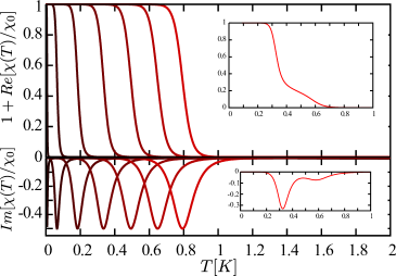
Figure 2: (color online) Superfluidity response as a function of the the Luttinger parameter $K$, which is determines the compressibility of the 1D fluid. $K$ ranges from 3.2 (dark) to 10.2(bright) ($\Delta k_{10}=0.001a^{-1}_{0}$, and $\Delta k_{11}/\Delta k_{10}=0.7$). The insets ($K=6.2$) show the effect of a larger value of the PS momenta ($\Delta k_{10}=0.5a^{-1}_{0}$ and $\Delta k_{11}/\Delta k_{10}=0.7$), resulting in the appearance of two dissipation peaks.

In ultracold atomic systems, the momentum response can be probed as described in Ref. Tokuno10 . Thus, here we restrict ourselves to discussing how the momentum response is probed by a torsional oscillator (TO). Our starting point is Newton’s equation of motion for a TO cell filled with liquid ⁴He:

$$\frac{d}{dt}\left[L_{z}(t)+\mathcal{L}_{z}(t)\right]=-\kappa\varphi(t)-\eta\dot{\varphi}(t)+\tau_{\mathrm{ext}}(t),$$ (4)

where $L_{z}(t)=I_{0}\dot{\varphi}(t)$ is the angular momentum and $I_{0}$ the moment of inertia of the empy TO, $\varphi(t)$ is the rotation angle, $\dot{\varphi}(t)=d\varphi(t)/dt$, $\kappa$ is the restoring torque per unit angle, $\eta$ the friction coefficient, and $\tau_{\mathrm{ext}}(t)$ the external torque driving the TO. $\mathcal{L}_{z}(t)$ is the angular momentum of the normal component of the helium sample (which is dragged along with the TO). Quantum mechanically, $\mathcal{L}_{z}(t)=\int d\mathbf{r}(\mathbf{\hat{z}}\times\mathbf{r})\cdot\langle\boldsymbol{\Pi}(\mathbf{r},t)\rangle$. For low rotation frequencies, this quantity can be computed within linear response theory: $\langle\Pi_{\mu}(\mathbf{r},t)\rangle=-\sum_{\nu}\int dtd\mathbf{r}^{\prime}\,\chi_{\mu\nu}(\mathbf{r},\mathbf{r}^{\prime},t-t^{\prime})\>(\dot{\varphi}(t^{\prime})\mathbf{\hat{z}}\times\mathbf{r}^{\prime})$ where $\chi_{\mu\nu}(\mathbf{r},\mathbf{r}^{\prime},t;T)$ is the momentum response of the liquid ⁴He in the TO cell at an absolute temperature $T$ convention . Hence, $\mathcal{L}_{z}(t)=-\int dt\,\chi_{n}(t-t^{\prime};T)\>\dot{\varphi}(t^{\prime})$ where $\chi_{n}(t;T)=\sum_{\mu,\nu}\int d\mathbf{r}d\mathbf{r}^{\prime}\,g_{\mu\nu}(\mathbf{r},\mathbf{r}^{\prime})\chi_{\mu\nu}(\mathbf{r},\mathbf{r}^{\prime},t;T)$ ($\mu,\nu=x,y,z$), and $g_{\mu\nu}(\mathbf{r},\mathbf{r}^{\prime})=\left(\mathbf{\hat{z}}\times\mathbf{r}\right)_{\mu}\left(\mathbf{\hat{z}}\times\mathbf{r}^{\prime}\right)_{\nu}$.The TO response is defined by the relationship $\varphi(t)=-\int dt\,\chi_{TO}(t-t^{\prime})\tau_{\mathrm{ext}}(t^{\prime})$. Hence, from (4),

$$\chi^{-1}_{TO}(\omega)=\omega^{2}\left[I_{0}-\chi_{n}(\omega;T)\right]+i\eta\omega-\kappa.$$ (5)

In Ref. Nussinov07 , the TO response has recently been discussed on phenomenological grounds. The expression reported there is identical to our Eq.(5) provided we identify $g(\omega;T)=-\omega^{2}\chi_{n}(\omega;T)$ where $g(\omega;T)$ is the back action function introduced in Ref. Nussinov07 . From (5) we see that the moment of inertia of the empty TO, $I_{0}$ is corrected by $\delta I_{n}=-\mathrm{Re}\>\chi_{n}(\omega;T)$ and the friction coefficient, is corrected by $\delta\eta_{n}=-\omega\mathrm{Im}\,\>\chi_{n}(\omega;T)$. To relate $\chi_{n}(\omega;T)$ to the momentum response of a 1D fluid computed above, we imagine a straight 1D channel located at $\mathbf{r}$, filled with liquid ⁴He, and oriented along the unit vector $\mathbf{\hat{d}}$. The momentum flow of the normal component is $\langle\boldsymbol{\Pi}(\mathbf{r},t)\rangle\propto\mathbf{\hat{d}}$ and the velocity of walls of the channel is $\mathbf{\hat{d}}\cdot\left(\mathbf{z}\times\mathbf{r}\right)\dot{\varphi}(t)$. For a typical sample size and TO oscillator driving frequencies ( $\sim 10^{3}$ Hz Taniguchi10 ) this velocity field varies very slowly on the scale of the length of the channel ($\sim 0.3\,\mu m$ Taniguchi10 ). Furthermore, we assume that finite-size effects can be neglected . Therefore, the momentum response of the channel is given by the $q=\mathbf{q}\cdot\mathbf{\hat{d}}\to 0$ limit of $\chi(q,\omega;T)$ computed for an infinite 1D system. However, besides the liquid ⁴He filling the 1D channel, there may be an additional contribution to $\chi_{n}(\omega;T)$ from other sources (in the experiment of Ref. Taniguchi10 these would correspond to liquid helium filling the cavities between the nanoporous pellets). We shall assume that, around the onset temperature, these contributions only provide a weakly temperature and frequency dependent background signal. Thus, $\chi_{n}(\omega;T)\simeq G_{0}\chi(\omega;T)+\mathrm{const.}$ where $G_{0}$ is a geometrical factor that measures the relative weight of the 1D channel network to the total response of the sample in the TO cell. Hence, the change in frequency of the TO is $\delta\omega(T)=\omega(T)-\omega_{+\infty}\sim G_{0}\left[1+\mathrm{Re}\>\chi(\omega_{0};T)/\chi_{0}\right]$, where $\omega_{0}=\sqrt{\kappa/I_{0}}$ and is the empty TO frequency (we neglect the difference between the TO resonance frequency and $\omega_{0}$ and $\omega_{+\infty}=\sqrt{\kappa/(I_{0}+G_{0}\chi_{0})}$, where $\chi_{0}=-\lim_{T\to 0}\lim_{\omega\to 0}\chi(\omega;T)=M^{2}vK/\pi\hbar$. The change in the quality factor is $\delta Q(T)\sim-G_{0}\>\mathrm{Im}\chi(\omega;T)$. Note that $G_{0}$ accounts for the distribution of orientations of the channels within the TO cell. Indeed, within the TO cell some 1D channels will be oriented perpendicular to flow of the walls (that is, $\mathbf{\hat{d}}\cdot\left(\mathbf{z}\times\mathbf{r}\right)\simeq 0$) and will not contribute to the change in the moment of inertia.

Finally, let us briefly discuss the relevance of our results for the observed supersolid behavior in solid ⁴He BalibarNature ; Supersolid . It has been suggested that in samples consisting of single crystals an explanation of of the observed supersolidity Supersolid ; BalibarNature are edge dislocations. Indeed, associated with the onset of superfluidity in this system, there is a prominent dissipation peak and a stiffening of the crystals. The latter is believed to be related of the pinning of dislocations by ³He impurities BalibarNature . At sufficiently low temperatures, the pinned dislocations become straight and behave as 1D superfluid channels Boninsegni07 that can be described as Tomonaga-Luttinger liquids with $K\simeq 5$ . The results reported here are fully applicable to such systems and improve on earlier theoretical treatments Shevchenko09 ; Boninsegni07 . Experimentally, it may be also interesting to further investigate the similarities in the TO response between the nanopore systems Toda07 ; Taniguchi10 and the supersolid behavior of ⁴He single crystals.

To summarize, we have reported a dynamical theory of superfluidity in 1D quantum fluids, showing that in 1D superfluidity is essentially a dynamical phenomenon related to the suppression of quantum PS at low temperatures. Our calculations go beyond previous theoretical treatments by computing the experimentally accessible dynamical momentum response of the 1D fluid which has been obtained in a particular case using the memory matrix formalism, allowing us to take into account the dynamical coupling between the particle and energy currents. We have also demonstrated the explicit relation between this response function to the measurable parameters of the torsional oscillator.

We thank M. Suzuki and J. Taniguchi for enlightening discussions on their TO experiments with liquid ⁴He in 1D. MAC gratefully acknowledges the hospitality of ISSP (University of Tokyo) and financial support from Spanish MEC grant FIS2010-19609-C02-02. MAC and TE thank D. W. Wang for his hospitality at NCTS (Taiwan). TE acknowledges support by a MEXT scholarship (Japan). The present work was partially carried out at the Supercomputer Center, ISSP, University of Tokyo.

Appendix A Supplementary Material

The helicity modulus

The helicity modulus Helicitymod is defined as $\Upsilon(T)=\lim_{L\to+\infty}\Upsilon(T,L)$ where $\Upsilon(T,L)=L\left(\partial^{2}F(\varphi,L,T)/\partial\varphi^{2}\right)\big{|}_{\varphi=0}$, where $F(\varphi,T,L)$ is the free energy computed with twisted boundary conditions on the field operator: $\Psi(x+L)=e^{i\varphi}\>\Psi(x)$. For a 1D system described by the TLL Hamiltonian $H_{0}$ it holds that

$$\Upsilon(T,L)=\Upsilon_{0}\left(1+\frac{\epsilon_{0}}{k_{B}T}\frac{\vartheta^{\prime\prime}_{3}(0,e^{-2\epsilon_{0}/k_{B}T})}{\vartheta_{3}(0,e^{-2\epsilon_{0}/k_{B}T})}\right)$$ (6)

where $\vartheta_{3}(z,q)=\sum_{n=-\infty}^{+\infty}q^{n^{2}}\>e^{2niz}$ is a Jacobi theta function, and $\vartheta^{\prime\prime}_{3}(z,q)=\frac{d^{2}\theta_{3}(z,q)}{dz^{2}}$, $\Upsilon_{0}=\hbar vK/\pi$ and $\epsilon_{0}=\hbar\pi vK/L$, where $vK$ is the phase stiffness at $T=0$. $\Upsilon(L,T)$ displays an onset at $T\sim\epsilon_{0}\sim L^{-1}$. Hence in the infinite system size limit

$$\Upsilon(T)=\lim_{L\to+\infty}\Upsilon(L,T)=0$$ (7)

excluding the possibility of a non-vanishing static superfluid density. For a pore of $R=2.8$ nm and lenght $L=0.3\,\mu\mathrm{m}$ Taniguchi10 , we find that when we subtract the inert layer on the inside of the pores that does not contribute to the superflow Toda07 , at most $T_{\mathrm{onset}}\simeq 0.18$ K, which seems too low when compared to the experimentally measured $T_{\mbox{\scriptsize onset}}\simeq 0.65$ K at a pressure of about 0.9MPa Taniguchi10 .

The memory matrix

As defined in the main text, the momentum response can be written in the memory matrix formalism Forster ; Giamarchi91 ; RoschAndrei in the following way:

$$\chi(\omega;T)=\mathrm{Tr}\left\{V\left[\omega 1+iM(\omega;T)\right]^{-1}iM(\omega;T)\boldsymbol{\chi}(T)\right\},$$ (8)

where $\boldsymbol{\chi}(T)\simeq\mathrm{diag}\{\chi_{JJ},\chi_{PP}(T)\}=\mathrm{diag}\{-\frac{M^{2}vK}{\hbar\pi},-\frac{\pi(k_{B}T)^{2}}{6\hbar v^{3}}\}$ is the matrix of static susceptibilities and the memory matrix, $M(\omega;T)$ computed to lowest order in $H_{irr}$ takes the form

$$M(\omega;T)\simeq\sum_{n>0,m}\frac{\hbar^{2}g^{2}_{nm}}{4\pi^{2}a^{4}_{0}}D_{nm}(\omega;T)U_{mn}\boldsymbol{\chi}^{-1}(T)$$ (9)

where

$$U_{mn}=\left(\begin{array}[]{cc}\left(\frac{2nMvK}{\hbar}\right)^{2}&-\frac{2nMvK}{\hbar}\Delta k_{mn}\\ -\frac{2nMvK}{\hbar}\Delta k_{mn}&(\Delta k_{mn})^{2}\end{array}\right)$$ (10)

and

$$D_{nm}(\omega;T)=\left[F_{mn}(\omega;T)-F_{mn}(\omega=0;T)\right]/(i\omega)$$ (11)

where

$$F_{mn}(\omega) =-i\hbar^{-1}\int dx\int^{+\infty}_{0}dt\,e^{i\omega t-i\Delta k_{mn}x}\>C_{n}(x,t)\$$

$$=-\frac{2a^{2}_{0}\sin\left(\pi n^{2}K\right)}{\hbar v}\left(\frac{2\pi k_{B}Ta_{0}}{\hbar v}\right)^{2n^{2}K-2}$$

$$\quad B\left(\frac{n^{2}K}{2}-i\frac{\hbar(\omega+v\Delta k_{nm})}{4\pi k_{B}T},1-n^{2}K\right)$$

$$\quad\quad\times B\left(\frac{n^{2}K}{2}-i\frac{\hbar(\omega-v\Delta k_{nm})}{4\pi k_{B}T},1-n^{2}K\right)$$ (12)

being $O_{n}(x,t)=e^{-2in\phi(x,t)}$, and $C_{n}(x,t)=\langle[O^{{\dagger}}_{n}(x,t),O_{n}(0,0)\rangle_{0}$, and $B(x,y)$ is the Euler Beta function.

References

- (1) D. J. Bishop and J. Reppy, Phys. Rev. Lett. 40, 1727 (1979).
- (2) V. L. Berezinskii Sov. Phys. JETP 34, 610 (1972); J. M. Kosterlitz and D. J. Thouless, J. Phys. C 6, 1181 (1973).
- (3) M. E. Fisher, M. Barber, and D. Jasnow, Phys. Rev. A 8, 1111 (1973).
- (4) V. Ambegaokar, B. I. Halperin, D. R. Nelson, and E. Siggia, Phys. Rev. Lett. 40, 783 (1978).
- (5) R. Toda et al., Phys. Rev. Lett. 99, 255301 (2007).
- (6) J. Taniguchi, Y. Aoki, and M. Suzuki, Phys. Rev. B 82, 104509 (2010).
- (7) F. S. Cataliotti et al., Science 293, 5531 (2001).
- (8) C. D. Fertig et al., Phys. Rev. Lett. 94, 120403 (2005).
- (9) E. Kim and M. H. W. Chan, Nature 427, 225 (2004); Science 305, 1941 (2004); A. S. Rittner and J. Reppy, Phys. Rev. Lett. 97, 165301 (2006).
- (10) M. Boninsegni et al. Phys. Rev. Lett. 99, 035301 (2007).
- (11) D. V. Fil and S. I. Sevchenko, Phys. Rev. B 80, 100501(R) (2009).
- (12) S. Balibar, Nature (London) 464, 176 (2010). X. Rojas et al., Phys. Rev. Lett. 105, 145302 (2010).
- (13) F. D. M. Haldane, Phys. Rev. Lett. 47, 1840 (1981)
- (14) M. A. Cazalilla, J. Phys. B 37, S1 (2004); M. A. Cazalilla et al., arXiv:1101.5337 (2010).
- (15) T. Giamarchi, Quantum Physics in One dimension (Clarendon Press, Oxford, 2004).
- (16) T. Kinoshita, D. S. Weiss, Nature (London) 440, 900 (2006). M. Rigol et al., Phys. Rev. Lett. 98, 050405 (2007); M. A. Cazalilla, Phys. Rev. Lett. 97, 156403 (2006).
- (17) H. Castella, X. Zotos, and P. Prelovsek, Phys. Rev. Lett. 74, 972 (1995). X. Zotos, ibid 82, 1764 (1999).
- (18) V. Ambegaokar and J. Langer, Phys. Rev. 164, 498 (1967)
- (19) S. Khlebnikov, Phys. Rev. Lett. 93, 090403 (2004); Phys. Rev. A 71, 013602 (2005).
- (20) A. Tokuno and T. Giamarchi, report arxiv::1101.2469 (2010).
- (21) G. Baym, in Mathematical Methods in Solid State and Superfluid Theory, edited by R. C. Clark and G. H. Derrick (Oliver and Boyd, Edinburgh, 1969), p. 121.
- (22) The minus sign stems from the standard convention for retarded correlation functions (e.g. A. L. Fetter and J. D. Walecka, Quantum Theory of Many-Particle Systems, Dover Publications (New York, 2003). This convention differs by a minus sign from the one used in Ref. Forster .
- (23) A. del Maestro and I. Affleck, Physical Review B 82, 060515(R) (2010).
- (24) A. del Maestro, M. Boninsegni, and I. Affleck, Phys. Rev. Lett. 106, 105303 (2011). 11282 (2000).
- (25) Z. Nussinov, A. V. Balatsky, M. J. Graf, and S. A. Trugman, Phys. Rev. B 76, 014530 (2007).
- (26) D. Forster, Hydrodynamic fluctuations, broken symmetry, and correlation functions, W. A. Bejamin (Reading, MA, 1975).
- (27) T. Giamarchi, Phys. Rev. B 44, 2905 (1991).
- (28) A. Rosch and N. Andrei, Phys. Rev. Lett.85, 1092 (2000)
- (29) T. Eggel, M. A. Cazalilla, and M. Oshikawa (unpublished).
- (30) K. Yamashita and D. S. Hirashima, Phys. Rev. B 79, 014501 (2009).