Minimal dissipation theory and shear bands in biaxial tests

Abstract

True biaxial tests of granular materials are investigated by applying the principle of minimal dissipation and comparing to two dimensional contact dynamics simulations. It is shown that the macroscopic steady state manifested by constant stress ratio and constant volume is the result of the ever changing microscopic structure which minimizes the dissipation rate. The shear band angle in the varying shear band structures is found to be constant. We also show that introducing friction on the walls reduces the degeneracy of the optimal shear band structures to one for a wide range of parameters which gives a non-constant stress ratio curve with varying aspect ratio that can be calculated.

1 Introduction

Shear bands seem inevitable whenever granular material is subject to quasistatic deformation. The form and the position of these failure zones depend on the experimental setup Nedderman and sometimes even on the specific sample Desrues84 .

Classical continuum theories predict strain fields from the stresses of the material under load. Generally accepted constitutive relations are still missing for dense granular materials, not to mention a microscopic understanding of the parameters.

Therefore it is legitimate to approach the physics of shear bands from a radically simplified perspective in which one idealizes shear bands as strain field singularities and regards them as the basic dynamical quantities of the theory. This is the approach used in this paper where shear bands are dividing the granular material into domains which are rigidly displaced with respect to each other. The realized shear band configuration is determined using the principle of least dissipation Unger04 ; Unger07 .

We apply this method to the true biaxial tester Kadau06 ; Schwedes containing a non-cohesive granular material, where steady state flow can be observed. It allows the deformation of a granular medium in a brick shaped container with perpendicular, frictionless walls. This keeps the principal axes of the stress and strain tensors constant and aligned perpendicular to the container walls. We would like to find out what is the structure of the flow that allows for an apparent macroscopic steady state, and under what conditions can one predict the velocity field of the sample.

In this paper we present first some numerical simulation results on true biaxial tests to motivate the theoretical model, which is then solved for the setup with frictionless and later with frictional walls. Finally we test the predictions on the simulation results.

2 Simulation results

2.1 Definition of the system

In this paper we use distinct element simulations to study the shearing of frictional granular material in the so called true biaxial tester Kadau06 ; Schwedes , which consists of two fixed walls normal to the $z$ direction, stress controlled confining walls normal to the $x$ direction (normal stress $\sigma_{xx}$), and strain controlled compressing walls perpendicular to the $y$ direction (normal strain rate $\dot{\epsilon}_{yy}{<}0$).

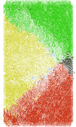
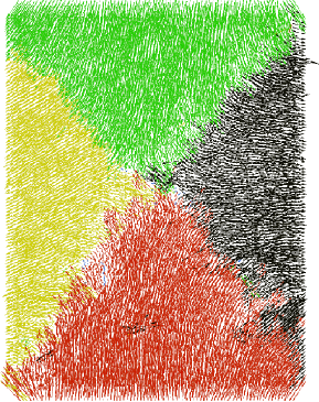
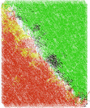
(a) (b) (c)

Figure 1: Snapshots from simulated biaxial tests. Time is progressing from (a) to (c). The particles are represented with arrows proportional to their actual velocity. The color (online) is given according to which quadrant the vector is pointing. Courtesy of D. Kadau Kadau06 .

The simulations were done using the contact dynamics method CD . Since the behavior is invariant along the $z$ direction we simulate only a two-dimensional system in the $xy$ plane. Samples of 10000 frictional discs were enclosed in a rectangle by four walls. For the constant confining stress $\sigma_{xx}$ on the vertical and compressing strain rate $\dot{\varepsilon}_{yy}$ on the horizontal walls we chose values such that the inertial number daCruz was always of the order of $10^{-4}$ Kadau06 so that the deformation can be regarded as quasistatic. Further details of the simulations can be found in Kadau06 . The particles were frictional with microscopic friction coefficient $\mu_{\mathrm{mic}}{=}0.3$. Tests with different particle numbers and friction coefficients show qualitatively identical results, and thus are not presented in this paper.

First, we present results with frictionless walls, corresponding to the usual experimental setup Schwedes .

2.2 Shear band patterns

For frictionless walls, after an initial transient, the stress $\sigma_{yy}$ measured on the strain controlled and the strain rate $\dot{\varepsilon}_{xx}$ on the stress controlled walls fluctuate around a constant value Kadau06 . This was interpreted as a steady state, however, the underlying microscopic behavior remains unknown.

On Fig. 1 we show some instantaneous velocity snapshots of a simulation at different instances. Visual observation of the velocity snapshots clearly indicate the existence of shear bands which are narrow straight lines reflected by the boundary or absorbed by the corners. In a different, two dimensional setup Hall et al. also reported complicated shear band structures Hall10 .

Simulations with different initial configurations show in general different shear band structures at given instances, however certain easily recognizable configurations appear around a given aspect ratio and never too far from it.

The above observations give rise to two important questions which we want to answer in this paper: (i) Why does the stress ratio $\sigma_{yy}/\sigma_{xx}$ remain constant in spite of the strongly varying velocity field, (ii) Is it possible to predict the shear band patterns in biaxial tests? In the next section we try to answer these questions based on the principle of minimal dissipation.

3 Principle of minimal dissipation

3.1 Theory

Before introducing the principle of minimal dissipation we summarize our assumptions: The system is described in the frame, where the center of mass is fixed at the origin. We assume that the sample has already reached steady state flow Pena06 and is quasistatic, i.e. there are no accelerations. Ignoring the small volume fluctuations allows the calculation of the velocities of all walls from the given strain rate $\dot{\epsilon}_{yy}$: The upper and lower walls move with velocity $-u_{y}$, respectively $u_{y}$, the left and right ones with $-u_{x}$, respectively $u_{x}$, where

$$u_{y}=L_{y}|\dot{\epsilon}_{yy}|/2\quad\mathrm{and}\quad u_{x}=L_{x}\dot{\epsilon}_{xx}/2=L_{x}|\dot{\epsilon}_{yy}|/2.$$ (1)

We model the shear bands as infinitely narrow, piecewise straight lines running all the way from one container wall to another without splitting or merging. These lines cut the system into domains inside which all grain velocities are the same. The domain boundaries are either shear band segments or walls.

The velocity of the particles in a domain must fulfill the following boundary conditions: (i) At a wall the normal component of a domain velocity must coincide with the velocity of the wall. The parallel component of the domain velocity can be freely chosen as the walls are frictionless. (ii) A shear band segment requires a discontinuity of the tangential velocity with some magnitude $\Delta v$, while the normal component must be continuous.

An immediate consequence of these two conditions is that shear bands cannot end at a wall, but must be “reflected” under some angle or end in one of the corners of the rectangular container. Thus, in the following we consider only shear band configurations represented by one or more piecewise straight paths ${\cal B}$ that close upon themselves or begin and end in a corner. Despite these restrictions the set of admissible shear band configurations is very large. They will be analyzed in detail in the next sections.

Among these possible configurations we select the ones which minimize the energy dissipation rate

$$\dot{E}=\int_{\cal B}\mu\Delta vPdl,$$ (2)

where the integral extends over the whole path ${\cal B}$ representing the shear band configuration, $\Delta v$ is the tangential velocity difference across the shear band, $P$ is the normal stress acting on the line element $dl$. We suppose that the material is homogeneous and is described by a single effective friction coefficient $\mu$ which is constant in the system.

3.2 Diagonal shear band

(a)   (b)

Figure 2: (a) The simplest shear band configuration, the diagonal. (b) Shear band configuration for $\alpha{=}\beta$ with one degree of freedom.

We start our analysis with the the simplest possible case which is a single shear band spanning diagonally the sample [Figs. 1(c) and 2(a)]. Let us denote the aspect ratio by $L_{y}/L_{x}{\equiv}\tan\beta$, the angle between the major principal axis (the $y$-axis in the present case) and the normal of the shear band by $\alpha$ (cf. Fig. 2). In this special case $\alpha{\equiv}\beta$.

The velocity in the two domains should match the bounding walls, so the velocity difference between the two domains is $\Delta v{=}u_{y}/\sin\alpha$. The unit length on the shear band is $dl{=}dx/\cos\alpha$. $P(\alpha)$ can be derived from force balance on the shear band as there are no accelerations: the horizontal components of the normal and tangential force components on the line element are $P(\alpha)dl\sin\alpha$ and $-\mu P(\alpha)dl\cos\alpha$, respectively. Their sum must be equal to $\sigma_{xx}dy$, where $dy/dl{=}\sin\alpha$, yielding

$$P(\alpha)=\frac{\sigma_{xx}}{1-\mu\cot\alpha}.$$ (3)

An immediate consequence is that the shear band angle $\alpha$ must be larger than the internal friction angle $\phi\equiv\arctan\mu$, as the normal stress cannot be tensile. When $\alpha$ approaches $\phi$ the normal stress $P$ diverges, expressing the impossibility that such a system moves (at finite confining stress $\sigma_{xx}$).

Thus the dissipation rate of the diagonal shear band takes the following form:

$$\dot{E}_{d}(\alpha) = \frac{\mu|\dot{\varepsilon}_{yy}|\sigma_{xx}V}{\cos\alpha\sin\alpha(1-\mu\cot\alpha)}$$ (4)

$$= \mu|\dot{\varepsilon}_{yy}|\sigma_{xx}V\frac{\tan^{2}\alpha+1}{\tan\alpha-\mu},$$ (5)

where $V{=}L_{x}L_{y}$ denotes the volume of the sample. Minimizing the above equation yields

$$\alpha_{\mathrm{min}}=\alpha_{\mathrm{MC}}=\frac{\pi}{4}+\frac{\phi}{2},$$ (6)

where $\alpha_{\mathrm{MC}}$ is the Mohr-Coulomb angle.

The equation (6) is an important result. It says that the dissipation rate for the diagonal shear band is minimal when the angle of the shear band equals to the Mohr-Coulomb angle.

The dissipation rate can be identified with the work per unit time done by the walls:

$$\dot{E}=-V\left(\sigma_{xx}\dot{\varepsilon}_{xx}+\sigma_{yy}\dot{\varepsilon}_{yy}\right)$$ (7)

From this the stress ratio can be derived:

$$s(\alpha)\equiv\frac{\sigma_{yy}}{\sigma_{xx}} = 1+\frac{\dot{E}}{|\dot{\varepsilon}_{yy}|\sigma_{xx}V}$$ (8)

$$= 1+\frac{\mu}{\cos\alpha\sin\alpha(1-\mu\cot\alpha)}$$ (9)

The stress ratio of this diagonal configuration varies with the aspect ratio. Thus the diagonal shear band should be observed only around $\beta\simeq\alpha_{\mathrm{MC}}$ otherwise the stress ratio cannot be constant.

3.3 Complex shear band structures

(a) (b)

Figure 3: Combined shear band configuration samples (a) $q/r=2/1$ (b) $q/r=3/2$. The arrows show the velocities of the particles in the domains.

Let us first examine the configuration shown on Fig. 2(b). For this configuration the formula for the dissipation rate is the same as in Eq. (4) since the length of the shear band is twice but the velocity jump is half than for the diagonal shear band. Thus again the minimum of the dissipation rate is at $\alpha{=}\beta{=}\alpha_{\mathrm{MC}}$.

Let us note, that Fig. 2(b) has a degree of freedom. The reflection point on the top wall can be anywhere. Moving the reflection point $R$ into the corner reduces this configuration to the diagonal shear band. Fig. 2(a) is a special case of Fig. 2(b).

Let us call shear band configuration Fig. 2(b) an elementary cell. More complicated shear band configurations can be constructed if we place $q$ times $r$ elementary cells in a rectangular lattice by matching the reflection point of the shear bands and scaling the velocity components to match at the cell boundaries (examples are shown in Fig. 3). The minimization presented in PG09 shows that for these configurations the dissipation rate is minimal if all shear band angles are equal and given by $\alpha{=}\alpha_{\mathrm{MC}}$. Furthermore the value of the dissipation rate is the same as for a single elementary cell (velocity jump and length scale inversely proportionally), namely:

$$\dot{E}_{\mathrm{min}}(\beta)=\dot{E}_{d}(\alpha_{\mathrm{MC}})$$ (10)

It is important to stress that the minimal dissipation rate for the complex shear band structures is independent of the values of $q$ and $r$.

On the other hand if $q/r{\not=}1$ then the aspect ratio of the sample is different from $\tan\alpha_{\mathrm{MC}}$. Thus for all aspect ratios $\tan\beta$ and for arbitrary small $\epsilon$ we can create a shear band configuration with $|q/r-\tan\alpha_{\mathrm{MC}}/\tan\beta|{<}\epsilon$ which have all the same $\dot{E}_{\mathrm{min}}$ with shear band angle equaling the Mohr-Coulomb angle.

The stress ratio is a linear function of the minimal dissipation rate cf. Eq. (8). Thus in the scope of this idealized theory at all aspect ratios we should find a different shear band configuration, and at the same time observe a constant stress ratio.

This constant stress ratio can be expressed with the effective friction coefficient $\mu$ cf. Eqs. (6) and (8):

$$s = \left(\mu+\sqrt{1+\mu^{2}}\right)^{2}$$ (11)

$$\mu = \tan\arcsin\left(\frac{s-1}{s+1}\right)$$ (12)

The above formula was already derived in a different way in Nedderman .

The stress ratio can be measured in the simulations to be $s{=}1.54$. From this value the effective friction coefficient gets $\mu{=}0.213$.

This result answers question (i) of Sec. 2.2. The apparent macroscopic steady state is the result of the complete lack of microscopic steady state which at each aspect ratio favors a different set of shear band configurations with the same minimal dissipation rate and stress ratio.

The answer for question (ii) is also clear within the scope of these idealized shear band structures: For all rational $\tan\alpha_{\mathrm{MC}}/\tan\beta$ there are infinitely many pairs of $q$ and $r$ that fulfill $\tan\alpha_{\mathrm{MC}}/\tan\beta{=}q/r$, and are equivalent in terms of dissipation rate. Thus it is impossible to predict which shear band configuration will be realized.

We should also note here PG09 that the linear nature of the system allows for linear combinations of shear band configurations which also enlarges the set of available configurations for a given aspect ratio. An example: Fig. 1 (b) is a linear combination of Fig. 1 (c) and its mirror image.

The results shown here are valid for homogeneous materials. In reality the effective friction coefficient fluctuates around its mean and does so the dissipation rate. The actual minimum does not only depend on the average value but also on the variance. The integral in Eq. (4) averages the fluctuations of the effective friction coefficient along the path. The overall variance of the path is inversly proportional to the length of the shear band. This way the shorter shear bands have larger variance and thus more likely to be minimal. A consequence is that one can easily find nice, simple shear band configurations like the examples on Fig. 1 in almost all simulations.

In summary in a perfectly homogeneous material one would find different shear band configurations at each time step. The apparent macroscopic steady state is the result of the fact that for the optimal configuration the dissipation rate depends only on the shear band angle and is independent of the aspect ratio.

4 Numerical results with frictionless walls

4.1 Shear band detection

An important prediction of our theory is that the shear band angle is independent of the sample aspect ratio and equals to the Mohr-Coulomb angle $\alpha_{\mathrm{MC}}$. In order to test this result on the simulations we need to detect the position of the shear band. Many quantities were already introduced to measure the local shear intensity Fazekas07 . We found that for our purpose the best choice is the Frobenius norm of the gradient of the coarse grained velocity $\vec{v}$ (see Goldhirsch01 ), which is defined as follows:

$$I_{vg}\equiv||\nabla\vec{v}||^{2}=(\partial_{x}v_{x})^{2}+(\partial_{x}v_{y})^{2}+(\partial_{y}v_{x})^{2}+(\partial_{y}v_{y})^{2}$$ (13)

The strain rate tensor can be decomposed into volumetric $\dot{\varepsilon}^{V}$ and shear $\dot{\varepsilon}^{S}$ strain part:

$$\dot{\varepsilon}_{ij} = \frac{\partial_{i}v_{j}+\partial_{j}v_{i}}{2}=$$ (14)

$$= \underbrace{\frac{\dot{\varepsilon}_{xx}+\dot{\varepsilon}_{yy}}{2}\delta_{ij}}_{\dot{\varepsilon}_{ij}^{V}}+\underbrace{\dot{\varepsilon}_{ij}-\frac{\dot{\varepsilon}_{xx}+\dot{\varepsilon}_{yy}}{2}\delta_{ij}}_{\dot{\varepsilon}_{ij}^{S}},$$ (15)

which leads to a decomposition of

$$I_{vg}=2\lambda_{\pm}^{2}+\frac{1}{2}\left(\dot{\varepsilon}_{xx}+\dot{\varepsilon}_{yy}\right)^{2}+\frac{1}{2}(\nabla\times\vec{v})^{2},$$ (16)

where $\lambda_{\pm}=\pm\sqrt{{\dot{\varepsilon}^{S}_{xx}\hbox{}}^{2}+{\dot{\varepsilon}^{S}_{xy}\hbox{}}^{2}}$ are the eigenvalues of the shear strain tensor.

In this paper we call $I_{vg}$ the local shear intensity.

4.2 Shear band direction

In general the angular correlation of $I_{vg}$ is a good way to measure the direction of the shear bands marked with high values of $I_{vg}$. However, in our case both $\alpha$ and $\pi{-}\alpha$ angle shear bands are possible that cross each other many times. This adds a lot of noise to the angular correlations. Thus we chose another method:

In order to measure the directions of the shear bands a segment $\vec{l}$ of length $l{=}|\vec{l}|$ larger than the width of the shear band is placed at point $\vec{x}$. Then the correlation between the local shear intensity is calculated at the end points of the segment only if all along the segment $\vec{l}$ the valus of $I_{vg}$ are larger than its average $\bar{I}_{vg}$. Thus the new angular correlation function is defined as:

$$C_{I}(\alpha,l)\equiv\langle I_{vg}(\vec{x})I_{vg}(\vec{x}+\vec{l})\rangle_{\vec{x},I_{vg}>\bar{I}_{vg}},$$ (17)

This definition has the advantage that it avoids contributions from points lying in different shear band segments.

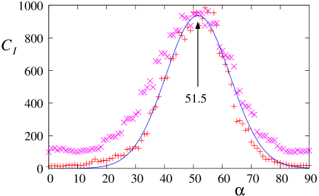
Figure 4: The segment angular correlation function of the shear intensity averaged for 4 samples and 400 timesteps, for $2.6{>}\tan\beta{>}0.5$. The length of the segment was $|\vec{l}|{=}10$ ($\times$), resp. $|\vec{l}|{=}12$ ($+$) in units of average particle diameter. The continuous curve is a Gaussian fit to the latter data for points $C_{I}{>}500$.

On Fig. 4 we show the values of $C_{I}$ for two different segment length. It displays a strong peak at an angle of $\alpha_{\mathrm{MC}}{=}51.5^{o}\pm 1^{o}$. The predicted value from the measured stress ratio is $\alpha_{\mathrm{MC}}{=}51^{o}$.

As a side result, the distribution functions predict a shear band width of about $6.5$ particle diameters, which is consistent with the picture of narrow shear bands.

5 Frictional walls

5.1 The X shaped shear band structure

The negative answer to the question (ii) of Sec. 2.2 raises another problem of importance. Namely: Is there a case where the principle of minimal dissipation can predict the observed shear band configuration? The answer can only be affirmative, if we can reduce the degeneracy of the possible solutions.

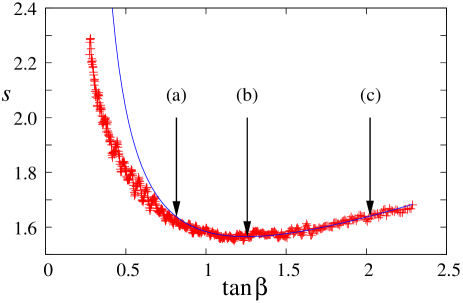
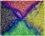
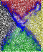
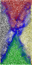
(a) (b) (c)

Figure 5: In the top figure the data points show the stress ratio as function of the angle of the diagonal. The data points are ensemble averages over 30 different realizations. The fitted curve is Eq. (8) with $\mu=0.226$. The snapshots presented below were taken at the indicated instances. The blue color is proportional to the shear intensity $I_{vg}$. Particles are color coded according to the quarter they are pointing to: red-north, yellow-east, green-south, black-west.

The simplest way to do this is to introduce friction on the walls. Wall friction introduces a finite difference in the dissipation rate for shear band configurations with or without velocity slip at the walls. Furthermore, it is obvious that there is only one shear band configuration with no tangential velocity at the walls, since the following two restrictions must be met: (i) it may not have any shear band reflected at the walls, which would mean different tangential velocities in the two domains, (ii) domains touching different walls should be separated by shear bands. These two conditions imply that perpendicular velocities in the domains touching the walls are only possible for the X-shaped shear band configuration, which is composed of the two diagonal shear bands, see Fig. 1(c).

We expect thus that the stress ratio is not constant any more but has a minimum at aspect ratio of the Mohr-Coulomb angle ($\tan\beta{=}\tan\alpha_{\mathrm{MC}}$) which is the optimal for the X-shaped shear band structure: Furthermore close to this point the stress ratio should be described by Eq. (8).

The above equation can be tested on our data. Since $\dot{\varepsilon}_{yy}$ is a simulation parameter, the only fit parameter we are left with is the effective friction coefficient of the bulk $\mu$. The value $\mu=0.226$, Eq. (8) fits very well the numerical data over a wide range of aspect ratios as shown on Fig. 5. Moreover snapshots of the system also clearly indicate the X-shaped shear band structure.

The difference between the friction coefficients in case of frictionless and frictional walls will be the subject of a future paper.

The answer to the question raised at the beginning of this section is thus yes, indeed there are cases when the principle of minimal dissipation is capable of predicting the actually observed shear bands. In the next section we discuss if we can predict the overall stress ratio curve and the other observed shear band configurations.

5.2 Complex shear band structures

The calculation of the dissipation rate for a general configuration in case of frictional walls is more complicated because pressure acting on shear band segments does not only depend on the shear band angle. Instead it must be calculated from the force balance of the domains. On Fig. 6 we show an example using the diagonal shear band.

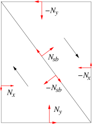
Figure 6: The forces acting on the domains in case of the diagonal shear band.

The force balance shown on Fig. 6 has one external parameter, the normal force $N_{x}{=}\sigma_{xx}L_{y}$ acting on the confining walls, two material parameters: the effective friction coefficient of the bulk $\mu$ and the wall friction $\mu_{w}$, and two unknowns, the normal force on the shear band $N_{sb}$ and the normal force on the compressing walls $N_{y}{=}\sigma_{yy}L_{x}$. The force balance of the two domains gives four (two components for each domain) linear equations for the unknowns, but for symmetry reasons only two are independent. The solution of these linear equations allows the calculation of the dissipation rate and the stress ratio.

The above process sounds simple, but in general it has many problems. First, in all cases there are more equations than unknowns and it may happen that a given shear band configuration often seen in the frictionless simulations gets realizable only at a given aspect ratio. Second, the analytic solution of the linear system of equations is of course possible, but the general analytic minimization is impossible due to the trigonometric functions. So we are left with analyzing numerically the candidate configurations one by one.

Instead of testing this infinite set of configurations - motivated by the typical shear band structure shown on Fig. 7 - we define here an incomplete shear band configuration in which only part of the shear band system is explicitely defined but still the minimization can be carried out. Here we focus on the aspect ratio range of $\beta\ll\alpha_{\mathrm{MC}}$ where the X shaped shear band becomes unfavourable.

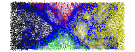
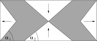
Figure 7: Top: A typical shear band structure beyond the X shape limit. Bottom: The schematic representation of the incomplete shear band structure.

Our assumptions are the following: (i) In order to minimize slip on the walls the generic configuration must have perpendicular velocities on the largest possible surface: This gives an X shape in the middle and two half X on the side walls. Since we are in the aspect ratio regime $\tan\beta{<}1$, the half X shear bands on the confining walls can cover the whole wall with an optimal angle $\alpha_{1}{=}\alpha_{\mathrm{MC}}$. The middle X does not cover the whole wall and it has an angle of $\alpha_{2}$ which does not necessarily match the Mohr-Coulomb angle. (ii) The structure in the place left out (gray parts on Fig. 7) remains unknown. We know however, that the force balance is kept on the known shear band segments. (iii) The velocity slip on the horizontal walls in the gray section is also unknown. Here we assume a simple linear dependence which gives an average slip velocity of $u_{x}/2$. Finally, we note here, that the visual observations fully support the above assumptions as shown on Fig. 7.

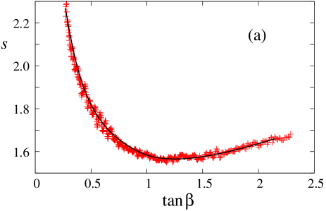
Figure 8: Test of the incomplete X configuration on the numerical data.

The minimization with respect to $\alpha_{2}$ of the dissipation rate for each aspect ratio is numerically possible if we know the effective wall friction coefficient. The latter parameter can be determined e.g. from simple shear simulations Zahra and it was found to be $\mu_{w}{\simeq}0.12$. The result of numerical minimization at different aspect ratios match prefectly the simulation data as shown on Fig. 8.

Thus in conclusion the introduction of friction on the walls destroys the apparent macroscopic steady state but fixes the shear band structure for a large range of aspect ratios. The prediction of the stress ratio is still possible with the help of two parameters, the effective friction of the bulk and the wall. Beside the central regime we cannot predict the exact shear band structure just some features of it.

6 Conclusion

In conclusion, in this paper we applied the principle of minimal dissipation to the biaxial shear test. From a theory based on simple assumptions, in case of frictionless walls, we were able to show that the apparent macroscopic constant stress ratio is a surprising result of the permanent minimization of the dissipation rate. This is manifested by a changing shear band configuration with constant shear band angle which is equal to the Mohr-Coulomb angle. For each sample aspect ratios different shear band configurations are optimal, but the high degeneracy of these optimal configurations denies us the possibility to predict the observed shear band configurations.

The above degeneracy can be reduced to a single optimal configuration by introducing friction on the walls, in which case for a wide range of aspect ratios a single configuration is optimal which can be clearly observed in simulations. Knowing the optimal configuration, or at least the important characteristics of it allows us to predict the the macroscopic stress ratio.

7 Acknowledgement

The partial support by the German-Israeli-Foundation under grant number I-795-166.10/2003 and by the German Research Foundation via SFB 616 and Piko SPP. Part of this work was funded by the Péter Pázmány program (RET-06/2005) of the Hungarian National Office for Research and Technology. We also give special thanks to Dirk Kadau who carried out preliminary simulation work and Tamas Unger for the discussions.

References

- (1) R.M. Nedderman, Statics and Kinematics of Granular Materials, (Cambridge University Press 1992).
- (2) J. Desrues, Thèse de Doctorat es Science, USMG and INPG, Grenoble (1984).
- (3) T. Unger, J. Török, J. Kertész and D. E. Wolf, Phys. Rev. Lett. 92, 214301 (2004).
- (4) T. Unger, Phys. Rev. Lett. 98, 018301 (2007).
- (5) D. Kadau, D. Schwesig, J. Theuerkauf, D. E. Wolf, Gran. Mat. 8, 35 (2006).
- (6) J. Harder, J. Schwedes, Part. Charact. 2, 149 (1985).
- (7) M. Jean and J. J. Moreau, Unilaterality and dry friction in the dynamics of rigid body collections. In Proceedings of Contact Mechanics International Symposium, pages 31-48, (Presses Polytechniques et Universitaires Romandes, Lausanne, Switzerland 1992), J. J. Moreau, Eur. J. Mech. A-Solids 13, 93 (1994).
- (8) F. da Cruz, S. Emam, M. Prochnow, J.-N. Roux, F. Chevoir, Phys. Rev. E 72, 021309 (2005).
- (9) A. A. Peña, A. Lizcano, F. Alons-Marroqiun, H. J. Herrmann, Int. J. Numer. Anal. Meth. Geomech. 00, 1-12 (2006). and refs [17-22].
- (10) S. A. Hall, D. M. Wood, E. Ibraim, Granular Matter 12, 1-14 (2010).
- (11) J. Török, L. Brendel and D. E. Wolf, in Powders and Grains 09, ed. by M. Nakagawa, S. Luding (Melville New York 2009 AIP) p. 417.
- (12) S. Fazekas, J. Török, J. Kertész, Phys. Rev. E 75, 011302 (2007).
- (13) B. J. Glasser, I. Goldhirsch, Phys. Fluids 13, 407 (2001).
- (14) Z. Shojaaee, A. Ries, L. Brendel, D.E. Wolf, Rheological Transitions in Two- and Three-Dimensional Granular Media in: Powders and Grains 2009 (AIP CP 1145), eds: M. Nakagawa, S. Luding (AIP, Melville, New York), 519 (2009).
- (15) J. Török, T. Unger, D. E. Wolf, J. Kertész, Phys. Rev. E 75, 011305 (2007).