Estimation procedures for a semiparametric family of bivariate copulas

Abstract

In this paper, we propose simple estimation methods dedicated to a semiparametric family of bivariate copulas. These copulas can be simply estimated through the estimation of their univariate generating function. We take profit of this result to estimate the associated measures of association as well as the high probability regions of the copula. These procedures are illustrated on simulations and on real data.

Keywords: Copulas, nonparametric estimate, measures of association, high probability regions.

1 Introduction

The theory of copulas provides a relevant tool to build multivariate probability laws, from fixed margins and required degree of dependence. From Sklar’s Theorem [22], the dependence properties of a continuous multivariate distribution $H$ can be entirely summarized, independently of its margins, by a copula, uniquely associated with $H$. Several families of copulas, such as Archimedian copulas [8] or copulas with polynomial sections [20, 18] have been proposed. More recently, we proposed to give up the polynomial form to work with a semiparametric family of copulas [1]. This permits to increase the dependence degree and to preserve the dependence properties of copulas with polynomial sections without significantly complexifying the model. Furthermore, the family of copulas is generated as simply as Archimedian copulas, that is by an univariate function.
Among the numerous papers dedicated to the construction of copulas, very few of them propose some associated inference procedures. Besides, starting from data, it is very difficult to find ”Which copula is the right one?”, see [12] for a review on this problem in the financial modeling context. The first attempt to estimate copulas is achieved in [2] with the introduction of nonparametric estimates based on empirical copulas. A recent contribution to the nonparametric estimation of copula for time series is presented in [23]. An alternative approach is to choose a parametric family of copulas and to estimate the parameters by a maximum likelihood method [15]. Both approaches suffer from their own drawbacks. In the first case, a fully nonparametric estimate is likely to suffer from the so-called “curse of dimensionality”. It would have a high variance for large number of margins and moderate size of datasets. At the opposite, a parametric estimate can lead to a very high bias if the prior family of copulas is not appropriate. Restricting to Archimedian copulas, Genest & Rivest [9] proposed a semiparametric estimate. In this family, estimating the copula reduces to estimating the generating function. It is therefore realistic to consider a nonparametric estimate of this univariate function. Here, we show that, similarly, the estimation of a copula in the semiparametric family [1] can be simply achieved by estimating nonparametrically the univariate generating function. This permits to overcome the curse of dimensionality. We deduce of this estimator some statistical procedures for estimating the associated dependence coefficients and high probability regions.
In section 2, the expression of the considered semiparametric family of copulas is given and its basic properties are recalled. Section 3 is dedicated to the estimation of the generating function and of the dependence coefficients. In section 4, we address the problem of estimating high probability regions. All the proposed estimates are experimented on simulated samples in section 5 and on real data in section 6.

2 Definition and basic properties

Throughout this paper, we note $I=[0,1]$. A bivariate copula defined on the unit square $I^{2}$ is a bivariate cumulative distribution function with univariate uniform $I$ margins. Equivalently, it must satisfy the following properties :

(P1)

$C(u,0)=C(0,v)=0$, $\forall(u,v)\in I^{2}$,

(P2)

$C(u,1)=u$ and $C(1,v)=v$, $\forall(u,v)\in I^{2}$,

(P3)

$\Delta(u_{1},u_{2},v_{1},v_{2})=C(u_{2},v_{2})-C(u_{2},v_{1})-C(u_{1},v_{2})+C(u_{1},v_{1})\geq 0$, $\forall(u_{1},u_{2},v_{1},v_{2})\in I^{4}$, such that $u_{1}\leq u_{2}$ and $v_{1}\leq v_{2}$.

Let us recall that, from Sklar’s Theorem [22], any bivariate distribution with cumulative distribution function $H(x,y)$ and marginal cumulative distribution functions $F(x)$ and $G(y)$ can be written $H(x,y)=C(F(x),G(y))$, where $C$ is a copula. This result justifies the use of copulas for building bivariate distributions.
Here, we consider the semiparametric family of functions defined on $I^{2}$ by:

$$C_{\theta,\phi}(u,v)=uv+\theta\phi(u)\phi(v),\;\;\theta\in[-1,1],$$ (2.1)

where $\phi$ is a function on $I$. This family was first introduced in [21], chapter 3, and is a particular case of Farlie’s family [6]. It is extensively studied in [1]. In particular, the following basic lemma is proved:

Lemma 1

$\phi$ generates a parametric family of copulas $\{C_{\theta,\phi},\;\theta\in[-1,1]\}$ if and only if it satisfies the following conditions :

(i)

$\phi(0)=\phi(1)=0$,

(ii)

$|\phi(x)-\phi(y)|\leq|x-y|$ for all $(x,y)\in I^{2}$.

The function $\phi$ plays a role similar to the generating function in Archimedian copulas [8]. Each copula $C_{\theta,\phi}$ is entirely described by the univariate function $\phi$ and the parameter $\theta$, which tunes the dependence between the margins. For instance, $\phi(x)=x(1-x)$ generates the Farlie-Gumbel-Morgenstern (FGM) family of copulas [17], which contains all copulas with both horizontal and vertical quadratic sections [20]. Another example is $\phi(x)=x(1-x)(1-2x)$ which defines the parametric family of symmetric copulas with cubic sections proposed in [18], equation (4.4). Of course, it is also possible to choose $\phi$ so as to define new copulas, see section 5 for an example.

3 Estimation of the generating function

3.1 Preliminaries

Let $(X,Y)$ be a random pair from the cumulative distribution function $H(x,y)=C_{\theta,\phi}(F(x),G(y))$, where $F(x)$ and $G(y)$ are respectively the cumulative distribution functions of $X$ and $Y$. The estimation of the copula reduces to estimating the generating function $\phi$ and the parameter $\theta$. This estimation clearly suffers from an identifiability problem since, for instance, replacing $\phi$ by $\phi/\sqrt{\alpha}$ and $\theta$ by $\alpha\theta$ for any positive $\alpha$ leads to the same copula. When $\theta\neq 0$, introducing $s=\theta/|\theta|$ and $\psi=\sqrt{|\theta|}\phi$ yields

$$C_{\theta,\phi}(u,v)=C_{s,\psi}(u,v)=uv+s\psi(u)\psi(v),$$ (3.1)

where $\psi$ satisfies the conditions of Lemma 1 and $s\in\{-1,1\}$. The identifiability problem is not fully overcome with the new parameterization (3.1) since the sign of $\psi$ cannot be identified. Thus, we limit ourselves to the Positively Quadrant Dependent (PDQ) context. Recall that $X$ and $Y$ are PQD [14], section 2.1.1, if and only if

$$\forall(x,y)\in\mathbb{R}^{2},\;\;P(X\leq x,Y\leq y)\geq P(X\leq x)P(Y\leq y).$$

As shown in [1], theorem 3, $X$ and $Y$ are PQD if and only if

$$\theta>0\mbox{ and, either }\forall u\in I,\;\phi(u)\geq 0\mbox{ or }\forall u\in I,\;\phi(u)\leq 0.$$ (3.2)

If $(X,Y)$ are PQD, then the copula (3.1) can always be rewritten as:

$$C_{1,\psi}(u,v)=uv+\psi(u)\psi(v),$$ (3.3)

where $\psi$ is a non negative function satisfying the conditions of Lemma 1. In the following, we limit ourselves to the estimation of $C_{1,\psi}$, or equivalently to the estimation of $\psi$ in this context. We refer to section 7 for possible improvements of the estimation method.

3.2 Estimation of $\psi(w)$

Let $\{(x_{i},y_{i}),i=1,\dots,n\}$ a sample of $(X,Y)$ from the cumulative distribution function $H(x,y)$. The rank transformations $u_{i}=\mbox{Rank}(x_{i})/n$ and $v_{i}=\mbox{Rank}(y_{i})/n$ yield an approximate sample from the copula $C_{1,\psi}(u,v)$. The estimation of $\psi(w)$ relies on the pseudo-observations $w_{i}=\max(u_{i},v_{i})$, $i=1,\dots,n$ which have the common distribution function $C_{1,\psi}(w,w)=w^{2}+\psi^{2}(w)$. In order to obtain a regular estimated function, this estimate is written as a linear combination of a denombrable set ${\cal A}$ of functions:

$$\widehat{\psi}(w)=\sum_{k\in{\cal A}}a_{k}e_{k}(w).$$ (3.4)

The set of functions $\{e_{k}(w),\;w\in I,\;k\in{\cal A}\}$ need not to be orthogonal but the condition $e_{k}(0)=e_{k}(1)=0$ is required for all $k\in{\cal A}$ in order to ensure $\widehat{\psi}(0)=\widehat{\psi}(1)=0$, and thus to respect condition (i) of Lemma 1. Introducing $w_{1,n}\leq\dots\leq w_{n,n}$ the ordered statistics associated to the $w_{i}$, $i=1,\dots,n$, the coefficients $a_{k}$ are determined by the constrained least-square problem

$$\hat{a}=\arg\min\left\{\|Ma-b\|^{2},\;0\leq(Ma)_{i},\;-1\leq(M^{\prime}a)_{i}\leq 1,\;i=1,\dots,n\right\}$$ (3.5)

where $M$ and $M^{\prime}$ are two matrices such that $M_{i,k}=e_{k}(w_{i,n})$ , $M^{\prime}_{i,k}=e^{\prime}_{k}(w_{i,n})$ for $k\in{\cal A}$, $i\in\{1,\dots,n\}$, and $b$ is a vector defined by $b_{i}=(i/(n+1)-w_{i,n}^{2})^{1/2}$, $i\in\{1,\dots,n\}$. The minimization of $\|Ma-b\|^{2}$ ensures that for all $i=1,\dots,n$

$$\widehat{\psi}(w_{i,n})^{2}=C_{1,\psi}(w_{i,n},w_{i,n})-w_{i,n}^{2}\approx i/(n+1)-w_{i,n}^{2}.$$ (3.6)

The positivity conditions $0\leq(Ma)_{i}$ impose that $0\leq\widehat{\psi}(w_{i,n})$, and the bound conditions
$-1\leq(M^{\prime}a)_{i}\leq 1$ are interpreted as $|\widehat{\psi}^{\prime}(w_{i,n})|\leq 1$ which allows to fulfil Lemma 1(ii).
In practice, the optimization process provides reasonably sparse solutions, that is vectors $a$ with a moderate number of nonzero components.

3.3 Estimation of an association measure

Two measures of association between the components of the random pair $(X,Y)$ are usually considered [14], section 2.1.9. The Kendall’s Tau is the probability of concordance minus the probability of discordance of two random pairs $(X_{1},Y_{1})$ and $(X_{2},Y_{2})$ described by the same joint bivariate law $H(x,y)=C(F(x),G(y))$. It only depends on the copula:

$$\tau=4\int_{I^{2}}C(u,v)dC(u,v)\!-\!1.$$ (3.7)

The Spearman’s Rho is the probability of concordance minus the probability of discordance of two pairs $(X_{1},Y_{1})$ and $(X_{2},Y_{2})$ with respective joint cumulative law $H(x,y)$ and $F(x)G(y)$,

$$\rho=12\int_{I^{2}}C(u,v)dudv\!-\!3.$$

In [1], proposition 1, it is shown that, within the family (2.1), these two measures are equivalent up to a scale factor: $2\rho=3\tau$. Here, we focus on the Spearman’s Rho whose expression is in our family:

$$\rho=12\theta\left(\int_{I}\phi(u)du\right)^{2}=12\left(\int_{I}\psi(u)du\right)^{2}.$$

We then propose an estimate based on the estimate $\widehat{\psi}$:

$$\hat{\rho}_{\mbox{\tiny SP}}=12\left(\sum_{k\in{\cal A}}a_{k}\beta_{k}\right)^{2},$$ (3.8)

where we have introduced $\beta_{k}=\int_{I}e_{k}(u)du$. This integral can be calculated analytically or numerically by Simpson’s rule, depending on the complexity of the basis of functions. It is also possible to estimate $\rho$ in a nonparametric way by rescaling the empirical version of (3.7) introduced in [9] with the factor $3/2$ to obtain:

$$\hat{\rho}_{\mbox{\tiny NP}}=\frac{6}{n(n-1)}\sum_{i=1}^{n}\sum_{j=1}^{n}{\mathbf{1}}\{u_{j}<u_{i},\;v_{j}<v_{i}\}-\frac{3}{2},$$

where ${\mathbf{1}}\{.\}$ is the indicator function. The two estimates $\hat{\rho}_{\mbox{\tiny SP}}$ and $\hat{\rho}_{\mbox{\tiny NP}}$ are compared on simulations in section 5.

4 Estimation of high probability regions

4.1 The general problem

Let us recall the definition of a $p$-dimensional $\alpha$-quantile of a distribution $P$. Let ${\cal S}$ the class of Borel measurable sets of ${\mathbb{R}}^{p}$ and let $\lambda$ be the Lebesgue measure defined on ${\cal S}$:

$$Q_{\alpha}=\inf\{\lambda(S):P(S)\geq\alpha,\;S\in{\cal S}\},\;0<\alpha\leq 1.$$

Here, $Q_{\alpha}$ is the minimum volume $S\in{\cal S}$ that contains at least a fraction $\alpha$ of the probability mass. This is a particular case of the general quantile function introduced by Einmal and Mason [5]. A particular attention has been paid to the estimation of $Q_{1}$, the support of the distribution, from a sample $\{M_{1},\dots,M_{n}\}$ of ${\mathbb{R}}^{p}$. The early paper of Geffroy [7] takes place in the case $p=2$ and the considered supports are written

$$Q_{1}=\{(x,y)\in{\mathbb{R}}^{2}:0\leq x\leq 1~{};\;0\leq y\leq f(x)\},$$

where $f$ is an unknown function. More recently, smooth estimates of the frontier function $f$ have been proposed [11] and their extension to star-shaped supports has been studied [13]. Numerous works have been dedicated to the nonparametric estimate

$$\widehat{Q}_{1}=\bigcup_{i=1}^{n}B(M_{i},r_{n}),$$

where $B(M_{i},r_{n})$ is the ball of radius $r_{n}$ and centered at $M_{i}$, see for instance [4, 10]. In the latter paper, a partition based estimate is also proposed. Introducing $\{K_{i}\}_{i\geq 1}$ a partition of ${\mathbb{R}}^{2}$, the estimate is simply:

$$\widehat{Q}_{1}=\bigcup_{i,j}K_{i}{\mathbf{1}}\{M_{j}\in K_{i}\}.$$

In subsection 4.2, we propose an estimate of $Q_{\alpha}$, $\alpha<1$, when $P$ is a bivariate copula, with a similar principle. Subsection 4.3 examines the special case of the semiparametric family of copulas $\{C_{1,\psi}\}$. The estimation of such high probability regions is of particular interest for bivariate copulas since some dependence properties can be read on this graph, see [16]. To this end, introduce the two diagonal lines $\ell_{1}$: $v=u$ and $\ell_{2}$: $v=1-u$ of the unit square $I^{2}$. If the graph of $Q_{\alpha}$ is nearly symmetric with respect to both diagonals $\ell_{1}$ and $\ell_{2}$ then the copula models weakly dependent variates. On the contrary, if the graph is concentrated along $\ell_{1}$, then the copula models strongly positively dependent variates.

4.2 The algorithm

Let $\{I_{k},\;k=1,\dots,N\}$ be the equidistant $N$-partition of $I$ and $K_{k,\ell}=I_{k}\times I_{\ell}$ the associated $N\times N$ grid. Denote $\delta_{k,\ell}\in\{0,1\}$, $k=1,\dots,N$, $\ell=1,\dots,N$ a binary $N\times N$ array and introduce the estimate

$$\widehat{Q}_{\alpha}=\bigcup_{k,\ell}K_{k,\ell}{\mathbf{1}}\{\delta_{k,\ell}=1\},$$ (4.1)

where the $\delta_{k,\ell}$ are defined by the optimization problem

$$\min\frac{1}{N^{2}}\sum_{k=1}^{N}\sum_{\ell=1}^{N}\delta_{k,\ell},$$ (4.2)

under the constraints $\delta_{k,\ell}\in\{0,1\}$ and

$$\sum_{k=1}^{N}\sum_{\ell=1}^{N}\delta_{k,\ell}\widehat{P}(K_{k,\ell})\geq\alpha.$$ (4.3)

The quantity $\widehat{P}(K_{k,\ell})$ is an estimation of the probability $P(K_{k,\ell})$. The quality of the estimate $\widehat{Q}_{\alpha}$ strongly depends on the quality of this estimate. This is discussed in subsection 4.3. Let us note that (4.2) is equivalent to minimizing $\lambda(\widehat{Q}_{\alpha})$ and (4.3) corresponds to the constraint $P(\widehat{Q}_{\alpha})\geq\alpha$. This optimization problem can be solved with a simple algorithm. The first step consists to sorting the estimated probabilities $\widehat{P}(K_{k,\ell})$ in decreasing order to obtain the sequence $\tilde{P}_{\tau}$, $\tau=1,\dots,N^{2}$. The second step is the computation of the number of subsets of the partition which are going to be used:

$$J=\min\left\{j,\;\sum_{\tau=1}^{j}\tilde{P}_{\tau}\geq\alpha\right\}.$$

The last step is the selection of the $J$ first subsets: $\delta_{k,\ell}=1\mbox{ if }1\leq\tau(k,\ell)\leq J,$ which leads to the estimate (4.1).

4.3 Estimation of $P(K_{k,\ell})$

If no information is available on the distribution $P$, one can use the nonparametric estimate

$$\widehat{P}_{\mbox{\tiny NP}}(K_{k,\ell})=\frac{1}{n}\sum_{i=1}^{n}{\mathbf{1}}\{M_{i}\in K_{k,\ell}\}.$$

Now, restricting ourselves to the family $\{C_{1,\psi}\}$ allows to consider semiparametric estimates, which are much more accurate than the nonparametric one. Taking into account of (3.3), it follows that

$$P(K_{k,\ell}) = C_{1,\psi}\left(\frac{k}{N},\frac{\ell}{N}\right)-C_{1,\psi}\left(\frac{k-1}{N},\frac{\ell}{N}\right)-C_{1,\psi}\left(\frac{k}{N},\frac{\ell-1}{N}\right)+C_{1,\psi}\left(\frac{k-1}{N},\frac{\ell-1}{N}\right)$$

$$= \frac{1}{N^{2}}+\left(\psi\left(\frac{k}{N}\right)-\psi\left(\frac{k-1}{N}\right)\right)\left(\psi\left(\frac{\ell}{N}\right)-\psi\left(\frac{\ell-1}{N}\right)\right).$$

Thus, basing on section 3, the following semiparametric estimate can be introduced

$$\widehat{P}_{\mbox{\tiny SP}}(K_{k,\ell})=\frac{1}{N^{2}}+\left({\widehat{\psi}}\left(\frac{k}{N}\right)-{\widehat{\psi}}\left(\frac{k-1}{N}\right)\right)\left({\widehat{\psi}}\left(\frac{\ell}{N}\right)-{\widehat{\psi}}\left(\frac{\ell-1}{N}\right)\right).$$

The results using $\widehat{P}_{\mbox{\tiny SP}}$ and $\widehat{P}_{\mbox{\tiny NP}}$ are compared on simulations in the next section.

5 Simulation results

All the numerical experiments of this section have been conducted on the family of copulas generated by the set of functions

$$\forall k\geq 1,\;\;\psi_{k}(x)=1-\left(x^{k}+(1-x)^{k}\right)^{1/k},\;x\in I.$$ (5.1)

For the sake of simplicity, the resulting family of copulas will be denoted by $C_{k}(u,v)=C_{1,\psi_{k}}(u,v)$. This family is interesting since it can represent very different distributions:

• When $k=1$, $C_{1}(x,y)$ is the uniform distribution on the unit square $I^{2}$. The associated Spearman’s Rho is $\rho_{1}=0$.

• Letting $k\to\infty$, we obtain $\psi_{k}(x)\to\psi_{\infty}(x)=\min(x,1-x)$ for all $x\in I$. Thus, it appears that $C_{\infty}(x,y)$ is a mixture of two uniform distributions on the squares $[0,1/2]^{2}$ and $[1/2,1]^{2}$ with mixing parameter $1/2$. The associated Spearman’s Rho is $\rho_{\infty}=3/4$, the maximum value in the family (2.1).

• When $1<k<\infty$, we get a bivariate distribution “interpolating” between the two previous one. Up to our knowledge, it is not possible to calculate $\rho_{k}$ explicitly.

5.1 Simulation of data from the copula

The simulation method described in [19], p. 36 is used. First, two independent uniform samples $u_{i}$ and $t_{i}$, $i=1,\dots,n$ are simulated. Second, for each $i=1,\dots,n$, $v_{i}$ is computed such that

$$t_{i}=\frac{\partial}{\partial u}C_{k}(u_{i},v_{i}),$$

by a dichotomy procedure. The resulting sample $(u_{i},v_{i})$, $i=1,\dots,n$ has joint distribution function $C_{k}(u,v)$.

5.2 Estimation of the generating function

In this paragraph, we have chosen $n=100$. Starting from the sample $(u_{i},v_{i})$, $i=1,\dots,n$, the generating function is estimated using the procedure described in section 3. The chosen basis of functions is doubly-indexed by a scale parameter $s$ and a location parameter $\ell$:

$$e_{s,\ell}(x)=\sin\left(\frac{\pi}{2}(2^{s+1}x-\ell)\right){\mathbf{1}}\{2^{s+1}x\in[\ell,\ell+2]\},\;(s,\ell)\in{\cal A},$$ (5.2)

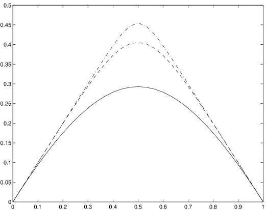
(a) True generating functions $\psi_{k}(x)$, $k\in\{2,4,8\}$

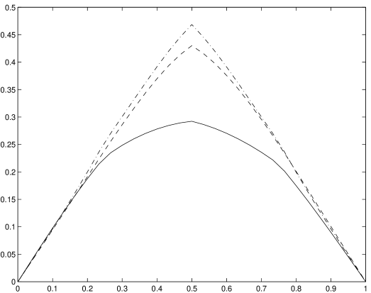
(b) Estimated generating functions $\hat{\psi}_{k}(x)$, $k\in\{2,4,8\}$

Figure 2: Comparison of the true generating functions $\psi_{k}(x)$ defined by (5.1) and the estimated ones $\hat{\psi}_{k}(x)$. Solid line: $k=2$, dashed line: $k=4$, dashdot line: $k=8$.

where ${\cal A}=\{(s,\ell),\;0\leq\ell\leq 2(2^{s}-1),\;0\leq s\}$. See figure 1 for a graph of the first basis functions. In figure 2, the estimation of $\psi_{2}(x)$, $\psi_{4}(x)$ and $\psi_{8}(x)$ is compared to the true generating functions. These first results are visually satisfying. The optimization procedure selects about 30 basis functions. A more precise comparison is achieved in table 1 by repeating each estimation on 100 different samples. On the basis of these 100 repetitions, the mean value and the standard deviation of the $L_{2}$ error

$$\varepsilon=\left(\int_{I}(\psi_{k}(x)-\hat{\psi_{k}}(x))^{2}dx\right)^{1/2}$$

are evaluated, as well as the mean value and the standard deviation of the two estimates $\hat{\rho}_{\mbox{\tiny SP}}$ and $\hat{\rho}_{\mbox{\tiny NP}}$ of the Spearman’s rho. The integral appearing in $\rho_{k}$ is calculated numerically using Simpson’s rule. The computation of $\hat{\rho}_{\mbox{\tiny SP}}$ is based on (3.8) and is thus explicit after remarking that $\beta_{s,\ell}=\int_{I}e_{s,\ell}(x)dx=2^{1-s}/\pi$.
The mean values of $\varepsilon$ (about $10^{-2}$) confirm that the function $\psi_{k}$ is correctly estimated. Moreover it appears that the semi parametric estimation of the Spearman’s Rho is better than the non parametric estimate, excepted for the case $k=1$. The standard deviations are similar for the two estimates.

5.3 Estimation of high probability regions

Starting from the estimations of $\psi_{2}(x)$, $\psi_{4}(x)$ and $\psi_{8}(x)$ obtained above, it is possible to estimate high probability regions $Q_{\alpha}$ with the procedure described in section 4. The following probabilities $\alpha=0.25$, $\alpha=0.5$ and $\alpha=0.75$ are considered. Here, the regions obtained using the semiparametric estimate $\widehat{P}_{\mbox{\tiny SP}}$, the nonparametric estimate $\widehat{P}_{\mbox{\tiny NP}}$ and the true probability $P$ can be compared. Of course, this probability depends on $\psi(x)$ and cannot be used in practical situations. Here $n=500$ and the estimated regions are obtained by a discretisation on a $N\times N$ grid with $N=30$ when using $\widehat{P}_{\mbox{\tiny SP}}$ or $P$ and $N=8$ when using $\widehat{P}_{\mbox{\tiny NP}}$ so as to obtain approximatively $500/64\simeq 8$ points in each cell. The results are presented on figures 3–5. It is apparent that the estimations obtained with the true probability $P$ and its semiparametric estimate $\widehat{P}_{\mbox{\tiny SP}}$ are very close, especially for moderate values of $k$. This confirms the results obtained in the previous paragraph. On the contrary, the nonparametric estimate accuracy is very poor for such values of the sample size $n$. We can also observe that, as $k$ increases, the high probability regions are more and more concentrated in the neighborhood of the $\ell_{1}$ diagonal line. This, together with table 1, illustrates the property that the positive dependence is increasing with $k$.

6 Real data

The dataset consists of $n=225$ countries on which two variables have been measured: $X$, the life expectancy at birth (years) in 2002 of the total population and $Y$, the difference between the life expectancy at birth of women and men. The data is available on the following web-site: http://www.odci.gov/cia/publications/factbook/. According to the PQD test proposed in [24], these data are PQD. The first step is to compute the rank transformations $u_{i}=\mbox{Rank}(x_{i})/n$ and $v_{i}=\mbox{Rank}(y_{i})/n$, see figure 7. Then, the generating function $\psi(x)$ is estimated using the basis (5.2). The optimization procedure yields an expansion of $\hat{\psi}(x)$ with respect to 24 basis functions. The function $\hat{\psi}(x)$ is plotted in figure 6. The estimated Spearman’s rho are $\hat{\rho}_{\mbox{\tiny NP}}=52.4\%$ and $\hat{\rho}_{\mbox{\tiny SP}}=40.7\%$. These values seem to confirm a moderate positive dependence between the two variables. The higher the life expectancy is, the more important the difference between women and men is. Finally, one can estimate the high probability regions. The same parameters as in the simulation section are used. The results are presented in figure 7. Of course, since the true function $\psi(x)$ is not known (and perhaps does not exist), it is only possible to compare the estimations obtained with the nonparametric and semiparametric estimates $\widehat{P}_{\mbox{\tiny NP}}$ and $\widehat{P}_{\mbox{\tiny SP}}$. The semiparametric estimation reveals two main groups of countries. In the first one, both men and women share a small life expectancy with weak differences between sexes. In the second one, both men and women share a large life expectancy but with important differences between sexes. The sample size is not large enough to obtain meaningful results with the nonparametric estimate.

7 Further work

We have presented a method for estimating copulas in the bivariate family of copulas $C_{s,\psi}(u,v)$ in the PQD case. Even though a test [3, 24] has not rejected the PQD assumption, deciding if the copula model $C_{s,\psi}(u,v)$ is adapted to a particular dataset is an opened problem. It could be possible to build a goodness-of-fit test based on the comparison of the estimations $\hat{\rho}_{\mbox{\tiny NP}}$ and $\hat{\rho}_{\mbox{\tiny SP}}$. The test would reject the model $C_{s,\psi}(u,v)$ if the difference $|\hat{\rho}_{\mbox{\tiny NP}}-\hat{\rho}_{\mbox{\tiny SP}}|$ is too large. If the PQD assumption is rejected, the proposed estimation method cannot be used. To overcome the identifiability problem, a possible modification of the method would be to replace the projection step (3.4) by the selection of the function $\psi$ in a database leading to the best approximation (3.6).

Figure 1: Graph of the first basis functions of (5.2). Solid line: $e_{0,0}(x)$, dotted line: $e_{1,0}(x)$, dashdot line: $e_{1,1}(x)$, dashed line: $e_{1,2}(x)$.

$$\begin{array}[]{|c|c|cc|cc|cc|}\hline\cr k&\rho_{k}&\mbox{mean}(\hat{\rho}_{\mbox{\tiny SP}})&\mbox{std}(\hat{\rho}_{\mbox{\tiny SP}})&\mbox{mean}(\hat{\rho}_{\mbox{\tiny NP}})&\mbox{std}(\hat{\rho}_{\mbox{\tiny NP}})&\mbox{mean}(\varepsilon)&\mbox{std}(\varepsilon)\\ &\times 10^{-2}&\times 10^{-2}&\times 10^{-2}&\times 10^{-2}&\times 10^{-2}&\times 10^{-2}&\times 10^{-2}\\ \hline\cr 1&0&0.81&(6.62)&0.18&(11.0)&8.75&(3.58)\\ 2&42.5&43.0&(9.91)&41.2&(9.11)&3.67&(1.26)\\ 4&66.4&65.8&(7.11)&64.3&(6.11)&3.01&(1.33))\\ 6&71.2&70.6&(7.60)&68.8&(6.09)&3.10&(1.35)\\ 8&72.8&72.1&(7.68)&70.2&(6.05)&3.10&(1.17)\\ \hline\cr\end{array}$$

Table 1: Estimation of the generating function and of the Spearman’s Rho ($\rho_{k}$). The mean value and the standard deviation of the $L_{2}$ error $\varepsilon$ as well as of the estimates $\hat{\rho}_{\mbox{\tiny SP}}$ and $\hat{\rho}_{\mbox{\tiny NP}}$ are evaluated on 100 repetitions.

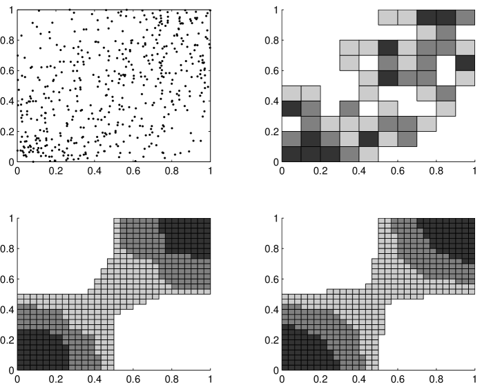
Figure 3: Estimation of high probability regions $Q_{\alpha}$ from $C_{2}(u,v)$. Dark Grey: $\alpha=0.25$, grey: $\alpha=0.5$, light grey: $\alpha=0.75$. Top left: simulated sample, top right: nonparametric estimate, bottom left: semiparametric estimate, bottom right: semiparametric estimate with the true function $\psi$.

Figure 4: Estimation of high probability regions $Q_{\alpha}$ from $C_{4}(u,v)$. Dark Grey: $\alpha=0.25$, grey: $\alpha=0.5$, light grey: $\alpha=0.75$. Top left: simulated sample, top right: nonparametric estimate, bottom left: semiparametric estimate, bottom right: semiparametric estimate with the true function $\psi$.

Figure 5: Estimation of high probability regions $Q_{\alpha}$ from $C_{8}(u,v)$. Dark Grey: $\alpha=0.25$, grey: $\alpha=0.5$, light grey: $\alpha=0.75$. Top left: simulated sample, top right: nonparametric estimate, bottom left: semiparametric estimate, bottom right: semiparametric estimate with the true function $\psi$.

Figure 6: Estimation of the generating function $\psi(x)$ from real data.

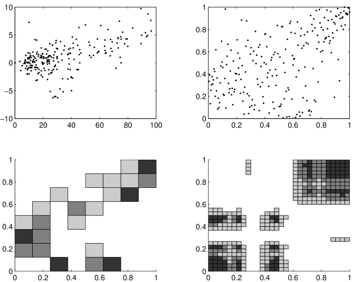
Figure 7: Estimation of high probability regions $Q_{\alpha}$ from real data. Dark Grey: $\alpha=0.25$, grey: $\alpha=0.5$, light grey: $\alpha=0.75$. Top left: real data, top right: real data after rank transformation, bottom left: nonparametric estimate, bottom right: semiparametric estimate.

References

- [1] Amblard, C. and Girard, S., 2002. Symmetry and dependence properties within a semiparametric family of bivariate copulas. Nonparametric Statistics, 14(6), 715–727.
- [2] Deheuvels, P., 1979. La fonction de dépendance empirique et ses propriétés. Un test non paramétrique d’indépendance. Bull. Cl. Sci., V. Ser., Acad. R. Belg., 65, 274–292.
- [3] Denuit, M. and Scaillet, O., 2004. Non parametric tests for positive quadrant dependence Journal of Financial Econometrics, to appear.
- [4] Devroye, L.P. and Wise, G.L., 1980. Detection of abnormal behavior via non parametric estimation of the support. SIAM J. Applied Math., 38, 448–480.
- [5] Einmal, J.H.J. and Mason, D.M, 1992. Generalized quantile process. The Annals of Statistics, 20(2), 1062–1078.
- [6] Farlie, D.G.J., 1960. The performance of some correlation coefficients for a general bivariate distribution. Biometrika, 47, 307–323.
- [7] Geffroy, J., 1964. Sur un problème d’estimation géométrique. Publ. Inst. Statist. Univ. Paris, XIII, 191–200.
- [8] Genest, C. and MacKay, J., 1986. Copules archimédiennes et familles de lois bidimensionnelles dont les marges sont données. Canad. J. Statist., 14, 145–159.
- [9] Genest, C. and Rivest, L., 1993. Statistical inference procedures for bivariate Archimedean copulas. Journal of the American Statistical Association, 88, 1034–1043.
- [10] Gensbittel M.H., 1979. Contribution à l’étude statistique de répartitions ponctuelles aléatoires. PhD Thesis, Université Pierre et Marie Curie, Paris.
- [11] Girard, S. and Jacob, P., 2003. Projection estimates of point processes boundaries. Journal of Statistical Planning and Inference, 116(1), 1–15.
- [12] Durrleman, V., Nikeghbali, A. and Roncalli, T., 2000. Which copula is the right one? Technical Report, Groupe de Recherche Opérationnelle Crédit Lyonnais.
- [13] Jacob, P. and Suquet, P., 1996. Regression and edge estimation. Statistics and Probability Letters, 27, 11–15.
- [14] Joe, H., 1997. Multivariate models and dependence concepts. Monographs on statistics and applied probability, 73, Chapman & Hall.
- [15] Joe, H. and Xu, J.J., 1996. The estimation method of inference functions for margins for multivariate models. Technical Report, 166, University of British Columbia.
- [16] Long, D. and Krzystofowicz, R., 1996. Geometry of a correlation coefficient under a copula. Commun. Statist.-Theory Meth., 25, 1397–1404.
- [17] Morgenstern, D., 1956. Einfache Beispiele Zweidimensionaler Verteilungen. Mitteilingsblatt f ur Matematische Statistik, 8, 234–235.
- [18] Nelsen, R. B., Quesada-Molina, J. J. and Rodríguez-Lallena, J. A., 1997. Bivariate copulas with cubic sections. Nonparametric Statistics, 7, 205–220.
- [19] Nelsen, R. B., 1999. An introduction to copulas. Lecture notes in statistics, 139, Springer.
- [20] Quesada-Molina, J. J. and Rodríguez-Lallena, J. A., 1995. Bivariate copulas with quadratic sections. Nonparametric Statistics, 5, 323–337.
- [21] Rodríguez Lallena, J. A., 1992. Estudio de la compabilidad y diseo de nuevas familias en la teoria de cópulas. Aplicaciones. Tesis doctoral, Universidad de Granada.
- [22] Sklar, A., 1959. Fonctions de répartition à dimensions et leurs marges. Publ. Inst. Statist. Univ. Paris, VIII, 229–231.
- [23] Scaillet, O. and Fermanian, J.D., 2003. Nonparametric estimation of copulas for times series, Journal of Risk, 5, 25-54.
- [24] Scaillet, O., 2004. A Kolmogorov-Smirnov type test for positive quadrant dependence, working paper, HEC Geneve.