Truncated Lévy Random Walks and Generalized Cauchy Processes

Abstract

A continuous Markovian model for truncated Lévy random walks is proposed. It generalizes the approach developed previously by Lubashevsky et al. Phys. Rev. E 79, 011110 (2009); 80, 031148 (2009), Eur. Phys. J. B 78, 207 (2010) allowing for nonlinear friction in wondering particle motion and saturation of the noise intensity depending on the particle velocity. Both the effects have own reason to be considered and individually give rise to truncated Lévy random walks as shown in the paper. The nonlinear Langevin equation governing the particle motion was solved numerically using an order 1.5 strong stochastic Runge-Kutta method and the obtained numerical data were employed to calculate the geometric mean of the particle displacement during a certain time interval and to construct its distribution function. It is demonstrated that the time dependence of the geometric mean comprises three fragments following one another as the time scale increases that can be categorized as the ballistic regime, the Lévy type regime (superballistic, quasiballistic, or superdiffusive one), and the standard motion of Brownian particles. For the intermediate Lévy type part the distribution of the particle displacement is found to be of the generalized Cauchy form with cutoff. Besides, the properties of the random walks at hand are shown to be determined mainly by a certain ratio of the friction coefficient and the noise intensity rather then their characteristics individually.

1 Introduction

Lévy random walks and Lévy flights are met in a large variety of systems different in nature (see, e.g. Mandl ; BG ; Biol1 ; Zasl1 ; Klaft1 ; ChBook ; RW1 ; RW7 ). In the strict mathematical sense, such Markovian stochastic processes are characterized by divergence of the second moment of walker displacement $x(t)$ for any time scale $t$, i.e., $\left<[x(t)]^{2}\right>\to\infty$, which is caused by power-law asymptotics of the distribution function $P(x,t)$. For example, in the 1D case it is $P(x,t)\sim Dt/x^{1+\alpha}$ for $x\gg(Dt)^{1/\alpha}$, where $D$ is some constant and the exponent $0<\alpha<2$ specifies the superdiffusion law usually written in a symbolic form as $\left<[x(t)]^{2}\right>\propto t^{\beta}$ with the exponent $\beta=2/\alpha>1$. Naturally, in the reality this divergence should be suppressed, for example, by the finite size of a system at hand. Thereby the given asymptotics can hold only within the frameworks of certain spatial and temporal scales bounded from below and above. The notion of truncated Lévy random walks (flights) takes into account the existence of these boundaries. To allow for such cutoff effects explicitly several approaches have been proposed. These include continuous-time random walks governed by the coupled spatial-temporal memory with finite moments CTRW1 ; CTRW2 , coupled continuous-time random walks with bounded variations in the velocity fluctuations CTRW3 , a direct cutoff in the Lévy noise Cutoff1 ; Cutoff2 , Lévy flights confined by external potentials Well1 , as well as Lévy flights damped by dissipative nonlinearity Checkin2005 .

Papers me1 ; me2 ; me3 developed a new approach to describing Lévy random walks based on continuous Markovian nonlinear stochastic processes. For example, in the 1D case it deals with random motion of a particle along the $x$-axis whose velocity $v$ obeys the following stochastic differential equation

$$\tau\frac{dv}{dt}=-\lambda v+\sqrt{2\tau(v_{a}^{2}+v^{2})}*\xi(t)$$ (1a)

written in the Hänggi-Klimontovich form, which is indicated with the multiplication symbol $$* \xi(t) \sqrt{2\tau(v_{a}^{2}+v^{2})} v \tau \lambda v_{a} \{v(t)\}$$ in the product of the white noise and the intensity of the Langevin forces depending itself on the particle velocity . Here is a certain “microscopic” time scale of the particle dynamics, is a friction coefficient, and the parameter actually quantifies the intensity of “additive” noise. Indeed, a time patterns with the same statistics can be generated using also the following stochastic differential equation

$$\tau\frac{dv}{dt}=-\left[\lambda+\sqrt{2\tau}\xi_{m}(t)\right]*v+\sqrt{2\tau}v_{a}\xi_{a}(t)$$ (1b)

explicitly containing additive, $\xi_{a}(t)$, and multiplicative, $\xi_{m}(t)$, noise Konno2007 . It should be noted that equation (1b) has been much employed to study stochastic behavior of various nonequilibrium systems, in particular, lasers K1 , on-off intermittency Nak5 , economic activity Nak9 , passive scalar field advected by fluid Nak11 , etc. Besides, appealing to qualitative arguments and a numerical example Sakaguchi Sak demonstrated that this equation can give rise to Lévy flights in the space $x$ on time scales $t\gg\tau$ if the random variable $v$ is regarded as the velocity $v=dx/dt$ of a Brownian particle.

Random walks generated by model (1a), on one hand, can be treated as continuous trajectories of particle motion and the corresponding probability density function $P(x,v,t)$ obeys the standard Fokker-Planck equation. It admits a conventional generalization taking into account possible medium heterogeneities as well as the existence of system boundaries via the appropriate boundary conditions. On the other hand, on time scales $t\gg\tau$ these random walks exhibit the characteristic properties, namely, the scaling law $\left<[x(t)]^{2}\right>\propto t^{\beta}$ and the power-law asymptotics of $P(x,v,t)$ as $x\to\infty$, that enable us to categorize them as Lévy random walks. It has been proved analytically for the superdiffusive regime ($1<\beta<2$) me2 and verified numerically for the quasiballistic and superballistic regimes ($\beta\geq 2$) me3 . So the given approach seems to make it possible to attack the yet unsolved problem of the formulation of accurate boundary conditions for the fractional Fokker-Planck equations describing Lévy processes in finite domains and heterogeneous media.

The purpose of the present paper is to generalize the developed approach in such a way that explicitly allows for not only the small scale cutoff of Lévy random walks determined actually by the parameter $\tau$ in the model at hand but also a large scale cutoff.

Generalized Cauchy processes

We employ generalized Cauchy processes for constructing a model for truncated Lévy random walks. There are several ways of introducing such stochastic processes starting from the Cauchy distribution

$$P_{C}(z)\propto\frac{1}{(\overline{z}_{t}^{2}+z^{2})}$$

of a random variable $z$, where $\overline{z}_{t}$ is a certain parameter which, in principle, can depend on time $t$ if, e.g., $\{z(t)\}$ is some stochastic process. In particular, Lim and Li LL following Gneiting and Schlather GS2004 focused their attention on anomalous relaxation phenomena and introduced generalized Cauchy processes appealing to a power-law decay in correlation functions. For example, the Cauchy distribution meets this interpretation when $\overline{z}_{t}\propto t^{\beta/2}$, because in this case $P_{C}(0)\propto t^{-\beta}$. Konno et al. Konno2007 ; Konno2011 related a generalization of Cauchy processes to a power-law asymptotics (maybe with some cutoff) of the distribution function $P(z)\propto|z|^{-\beta^{\prime}}$ when the analyzed random variable $z$ takes large values, $|z|\gg\overline{z}_{t}$. For the Cauchy distribution the equality $\beta^{\prime}=2$ holds. Below the term of the generalized Cauchy processes will be understood in the latter sense.

Let us discuss a modification of the Langevin equation (1a) within the introduction of a nonlinear friction, i.e., a friction coefficient $\lambda(v)$ depending on the particle velocity $v$ as well as the intensity $G(v)$ of the Langevin random forces depending on the particle velocity $v$ in a more complex way then it is accepted in model (1a). i.e., within the replacement

$$\lambda\rightarrow\lambda(v)\quad\text{and}\quad\sqrt{v_{a}^{2}+v^{2}}\rightarrow G(v)\,.$$ (2)

It should be pointed out that the introduction of nonlinear friction into a stochastic differential equation with additive Lévy noise gives rise to truncated Lévy flights Checkin2005 as well as the Langevin equation (1a) modified in the same way describes the generalized Cauchy process with a large scale cutoff Konno2011 .

Giving consideration to each of the two replacements has its own reason. First, the velocity dependence of friction coefficient is widely used in describing nonlinear dissipation processes in nonequilibrium systems and for the systems where the intensity of dissipation grows with particle velocity the Ansatz

$$\lambda(v)=\lambda_{0}+\lambda_{2}v^{2}$$ (3)

with the coefficients $\lambda_{0},\lambda_{2}>0$ is a simple and rather natural model for these phenomena (see, e.g., KlimontovichPOS ). Moreover, in describing motion of biological objects models assuming $\lambda(v)\propto|v|^{\beta^{\prime\prime}}$ are also met (see, e.g., Lindner2007 ). Appealing to Brownian motion governed by nonlinear friction and Lévy noise Checkin2005 we may expect that a model similar to (1a) with the friction coefficient (3) also generates truncated Lévy random walks on large time scales.

Second, the cutoff effect can be also due to the intensity $G(v)$ of the Langevin random forces reaching its saturation as the velocity $v$ increases. By way of example, let us mention movement of animals in searching for food resources, mates, den sites, etc. It has been found out that when animals have no information about the targets the resulting movement patterns of many species are of fractal, i.e., scale-free structure at least within multiple scales and can be described in terms of Lévy flights or truncated once (see, e.g., RW1 ; RW7 ). The complexity of the movement patterns is due to combination of various “behavioral modes” that change over time and, thus, this animal movement can be regarded as a composition of Gaussian random walks with the intensity changing in time Benhamou2007 (see also the following discussion BenhD1 ; BenhD2 ). To quantify the intensity of the current behavioral mode the magnitude $|\mathbf{v}|$ of the animal velocity $\mathbf{v}$ can be used as a natural parameter that aggregates in itself the ultimate stimuli to the given behavior. So in mimicking the animal motion patterns based on stochastic differential equations similar to (1a) the noise intensity $G(v)$ may be approximated by the Ansatz

$$G(v)=\sqrt{\frac{v_{a}^{2}+v^{2}}{1+\epsilon v^{2}}}\,.$$ (4)

It takes into account the low threshold in the animal perception of the optimal behavior as well as the animal bounded capacity of intensifying the search process quantified by the parameter $\epsilon$ such that $\epsilon v^{2}_{a}\ll 1$. Figure 1 illustrates dependence (4).

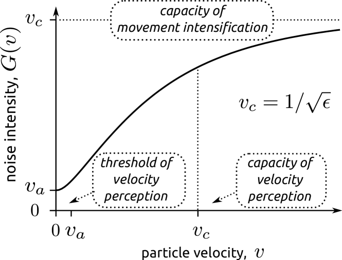
Figure 1: The characteristic dependence of the noise intensity on the particle velocity that mimics the animal behavior in foraging. It was used in constructing Ansatz (4).

For the stochastic process governed by equation (1a) within replacements (2) the probability distribution function $P(v,t)$ obeys the following Fokker-Planck equation

$$\tau\frac{\partial P}{\partial t}=\frac{\partial}{\partial v}\left\{G^{2}(v)\frac{\partial P}{\partial v}+v\lambda(v)P\right\}\,.$$ (5)

Its steady state solution, i.e., the stationary distribution $P^{\text{st}}(v)$ is of the form

$$P^{\text{st}}(v)=C\exp\left[-\int\limits_{0}^{v}\frac{u\lambda(u)}{G^{2}(u)}\,du\right]\,,$$ (6)

where $C$ is the normalization constant specified by the equality

$$\frac{1}{C}=2\int\limits_{0}^{\infty}\exp\left[-\int\limits_{0}^{v}\frac{u\lambda(u)}{G^{2}(u)}\,du\right]dv$$ (7)

stemming directly from the normalization of the distribution function $P^{\text{st}}(v)$ to unity.

In what follows we intend to analyze the two possible mechanisms of the cutoff individually. Namely, two alternative cases will be studied employing separately the former replacement of (2) or the latter one. In order to have some common “reference point” in comparing the cutoff effects caused by these mechanisms we will consider the models characterized by the same stationary distribution function. In other words, the parameters $\lambda_{0}$, $\lambda_{2}$, and $\epsilon$ will be set equal to such values that the ratio $\lambda(v)/G^{2}(v)$ be the same function in both the cases. In addition, to single out the key points of the models at hand let us convert to the dimensionless variables, namely,

$$t \rightarrow t\tau\,, x \rightarrow(v_{a}\tau)x\,, v \rightarrow v_{a}v\,.$$ (8)

Below all the results will be presented using these dimensionless time $t$, spatial coordinate $x$, and velocity $v$.

2 Model

Random walks $\{x(t)\}$ of a wandering particle in the 1D space $x\in\mathbb{R}$ are under consideration. The dynamics of its velocity $v=dx/dt$ is assumed to be governed by the following Langevin equation of the Hänggi-Klimontovich type

$$\frac{dv}{dt}=-(\alpha+1)vk(v)+\sqrt{2}g(v)*\xi(t)\,.$$ (9)

Here $\xi(t)$ is the white Gaussian noise with the correlation function

$$\left\langle\xi(t)\xi(t^{\prime})\right\rangle=\delta(t-t^{\prime})\,,$$ (10)

the value $0<\alpha<2$ is a model parameter and $k(v)>0$, $g(v)>0$ are certain positive definite smooth functions of the argument $v^{2}$ such that

$$k(0)=1\quad\text{and}\quad g(0)=1\,.$$ (11)

The numerical coefficient $\sqrt{2}$ has been introduced into (9) for the sake of convenience. In what follows the functions $k(v)>0$ and $g(v)>0$ will be referred to as the friction coefficient and the noise intensity, respectively, or just kinetic coefficients with respect to both of them.

When the kinetic coefficients are specified by the expressions

$$k_{0}(v)=1\quad\text{and}\quad g_{0}(v)=\sqrt{1+v^{2}}\,,$$ (12)

the stationary distribution function (6) which in the given case takes the form

$$P_{0}^{\text{st}}(v)=\frac{1}{B\left(\tfrac{1}{2},\tfrac{\alpha}{2}\right)\left(1+v^{2}\right)^{\tfrac{(1+\alpha)}{2}}}$$ (13)

exhibits power-law asymptotics and its second moment diverges for $\alpha\leq 2$. Here $B(\cdot,\cdot)$ is the Beta function. Under such conditions stochastic motion of this particle can be regarded as Lévy random walks on time scales $t\gg 1$ me1 ; me2 ; me3 . Moreover, for $\alpha\in(0,1)$ the generated Lévy random walks are of the superballistic type me3 , whereas for $\alpha\in(1,2)$ they are of the superdiffusive type me1 ; me2 . When $\alpha=1$ the stationary distribution function of the particle velocity is of the Cauchy form and the corresponding random walks can be treated as quasi-ballistic ones me3 .

As stated in Introduction, in the present paper the cutoff effects are related to deviation of the kinetic coefficients $k(v)$ and $g(v)$ from the ideal dependences $k_{0}(v)$ and $g_{0}(v)$. To be specific we will make us of the following Ansätze

$$k_{c}(v) =1+\frac{v^{2}}{v_{c}^{2}} g_{c}(v) =\sqrt{\frac{1+v^{2}}{1+v^{2}/v_{c}^{2}}}\,,$$ and (14)

where the parameter $v_{c}\gg 1$ is a certain critical value of the particle velocity when nonlinear effects responsible for the cutoff become essential.

Below we will consider in detail two cases,

$$\text{case I}\Rightarrow\begin{cases}k(v)=k_{c}(v)\\ g(v)=g_{0}(v)\end{cases}\!\!\!\text{and case II}\Rightarrow\begin{cases}k(v)=k_{0}(v)\\ g(v)=g_{c}(v)\end{cases}$$

which enables us, in particular, to elucidate the difference between the Lévy type random works generated by the stochastic process (9) when either the friction coefficient or the noise intensity gives rise to the cutoff. The case $k(v)=k_{0}(v)$ and $g(v)=g_{0}(v)$ will be also referred to as the unlimited Lévy random walks.

As intended, in the two cases the stationary distribution function (6) is of the same form

$$P_{c}^{\text{st}}(v)=\frac{C_{c}}{\left(1+v^{2}\right)^{\big{(}1-\tfrac{1}{v_{c}^{2}}\big{)}\tfrac{(1+\alpha)}{2}}}\,e^{-\tfrac{(1+\alpha)}{2}\left(\tfrac{v}{v_{c}}\right)^{2}}$$ (15)

with the normalization constant given by the expression

$$C_{c}=\left[\sqrt{\pi}U\left(\frac{1}{2},\frac{2-\alpha}{2}+\frac{(1+\alpha)}{2v_{c}^{2}},\frac{(1+\alpha)}{2v_{c}^{2}}\right)\right]^{-1}\,,$$ (16)

where $U(\cdot,\cdot,\cdot)$ is the confluent hypergeometric function of the second kind. Distribution (15) can be regarded as a generalized Cauchy distribution with cutoff whose characteristics are studied in detail in Ref. Konno2011 .

3 Results of numerical simulation

To analyze the statistical properties of random walks generated by model (9) it has been solved numerically using the SRI2W1 algorithm of the Runge-Kutta methords for strong approximation of stochastic differential equations of the Itô type with scalar noise Roussler . This algorithm has the deterministic order 3.0 and the stochastic order 1.5. Mersenne Twister algorithm by Matsumoto and Nishimura MTAlg implemented in GNU Scientific Library 1.14 GSL was used in generating random numbers. In integration the time step was set equal to $dt=0.01$, which gives stable results with respect to a decrease or increase of the time step by several times. The integration time was chosen to be equal to $T=10^{8}$ in order to accumulate enough statistics for analyzing the distribution tails based on individual trajectories, which enables us to avoid the problem of possible partial ergodicity of systems under consideration me3 . The created computer program was verified, in particular, by reproducing the velocity distribution function (15) numerically.

The obtained numerical data were used in order to analyze two characteristics. The first one is the geometric mean $\overline{x}_{g}(t)$ of the particle displacement $\delta_{t}x$ during the time interval $t$; it is defined via the formula

$$\ln\left[\overline{x}_{g}(t)\right]=\left<\ln\left(|\delta_{t}x|\right)\right>\,.$$ (17)

Here the angle brackets $\langle\ldots\rangle$ denote the time averaging, i.e., partitioning of a generated trajectory of length $T\gg t$ into fragments of duration $t$ and then averaging over the obtained fragments. In the given model for the unlimited Lévy random walks, i.e., for $v_{c}=\infty$ the asymptotics of the geometric mean $\overline{x}_{g}(t)$ as $t\to\infty$ can be written in the form me2 ; me3

$$\overline{x}_{g}^{L}(t)=\Lambda_{g}t^{1/\alpha}\,,$$ (18)

where the coefficient

$$\Lambda_{g}=\left[\frac{\Gamma\left(\dfrac{2-\alpha}{2}\right)}{2^{\alpha-1}\Gamma\left(\dfrac{\alpha}{2}\right)\Gamma(\alpha)}\right]^{\tfrac{1}{\alpha}}\exp\left[\gamma\frac{(1-\alpha)}{\alpha}\right]\,,$$ (19)

$\Gamma(\ldots)$ is the gamma function, and $\gamma\approx 0.5772$ is the Euler-Mascheroni constant.

The second characteristics is the probability density $P(\rho,t)$ of the particle displacement $\delta_{t}x$ during the time interval $t$ measured in units of the corresponding geometric mean, i.e., the random variable $\rho=\delta_{t}x/\overline{x}_{g}(t)$. Again this distribution density was constructed based on partitioning of a single sufficiently long trajectory. For the unlimited Lévy random walks the asymptotics of the probability density is known, namely, it is of the form me3

$$P_{L}(\rho)=\frac{2}{\pi}\sin\left(\frac{\pi\alpha}{2}\right)\Gamma(1+\alpha)e^{\gamma(\alpha-1)}\frac{1}{\rho^{1+\alpha}}$$ (20)

as $\rho\to\infty$ and does not depend on the time scale for $t\gg 1$.

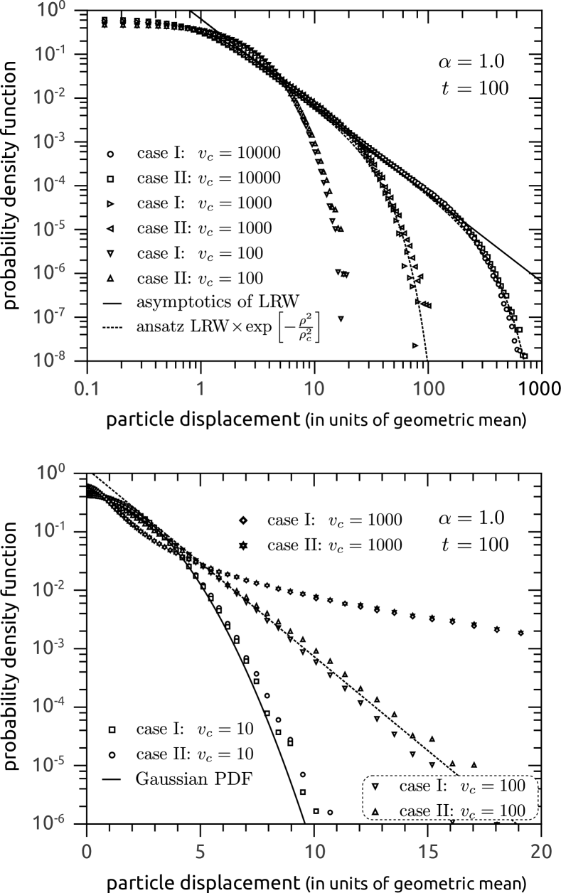
Figure 2: Probability density $P(\rho,t)$ as a function of the particle displacement normalized to the the corresponding geometric mean, $\rho(t)=\delta_{t}x/\overline{x}_{g}(t)$, for various values of the cutoff velocity $v_{c}$. The used values of the parameter $\alpha$ and the duration $t$ of the analyzed trajectory fragments are shown inside the frames.

Figure 2 shows the obtained results for the probability density $P(\rho,t)$. Appealing to this figure we can state the following. When the cutoff region is rather distant from the origin in the velocity space, i.e., the parameter $v_{c}$ is rather large, model (9) descries random walks for which the particle displacement $\delta_{t}x$ obeys the generalized Cauchy statistics with a certain cutoff. The solid line in the upper frame of Fig. 2 visualizes asymptotic (20) corresponding to the unlimited Lévy random walks. In this frame the dotted lines display the phenomenological Ansatz

$$P(\rho,t)\sim P_{L}(\rho)\exp\left[-\frac{\rho^{2}}{\rho_{c}^{2}}\right]\quad\text{as $\rho\to\infty$}\,,$$ (21)

where $\rho_{c}\approx 3.2\times 10^{2}$ and $\rho_{c}\approx 3.3\times 10$ for $v_{c}=10^{5}$ and $v_{c}=10^{3}$, respectively. The found magnitudes of the parameter $\rho_{c}$ validate the following construction of the relationship between the critical velocity $v_{c}$ and the characteristic scale $\Delta_{c}$ determining the cutoff region $\delta_{t}x\gtrsim\Delta_{c}$ in the space of the particle displacement $\{\delta_{t}x\}$.

As it is known me1 ; me2 , for the unlimited Lévy random walks there is a relation between the particle displacement $\delta_{t}x$ attained within a given trajectory fragment of duration $t\gg 1$ and the extreme fluctuations in the particle velocity within this fragment. Namely, the magnitude of $\delta_{t}x$ is mainly determined by motion of the particle during the peak of the corresponding time pattern $\{v(t^{\prime})\}$ with the maximal amplitude $v^{\text{max}}_{t}$. Since the characteristic time scale of such extreme velocity fluctuations is about unity (in dimensionless units), the proportionality $\delta_{t}x\sim cv^{\text{max}}_{t}$ with $c\sim 1$ holds. Moreover, the estimate

$$c=\left[\frac{2\sin\left(\dfrac{\pi\alpha}{2}\right)\Gamma\left(\dfrac{2-\alpha}{2}\right)}{\sqrt{\pi}\alpha\Gamma\left(\dfrac{\alpha+1}{2}\right)}\right]^{\tfrac{1}{\alpha}}$$ (22)

can be employed me1 and for $\alpha=1$ we have $c=2$. In particular, the geometric mean $\overline{x}_{g}(t)$ actually evaluates the characteristic amplitude of these extreme peaks gained by the particle velocity during the time interval $t$, i.e., $c\langle v^{\text{max}}_{t}\rangle\sim\overline{x}_{g}(t)$ me2 ; me3 .

The cutoff effect in the statistics of the particle displacement has to become pronounced when the amplitude of extreme velocity fluctuations gets the cutoff region in the velocity space, $v^{\text{max}}_{t}\sim v_{c}$. It immediately enables us to write the desired relationship

$$\Delta_{c} \sim cv_{c}\,,$$ (23a)

in the used notations it becomes

$$\rho_{c}(t)\cdot\overline{x}_{g}(t) \sim cv_{c}\,.$$ (23b)

According to the results to be presented below as well as obtained in Ref. me3 , the estimate $\overline{x}_{g}(t)\approx 100$ holds for the unlimited Lévy random walks when the parameter $\alpha=1$ and the time scale $t=100$. The found magnitudes for the quantity $\rho_{c}$ and the geometric mean $\overline{x}_{g}$ together with the values of the parameter $v_{c}$ used in the numerical simulations fit estimate (23b) very well, justifying the given arguments.

As the time scale $t$ increases the intermediate region matching the Lévy type asymptotics (20) should shrink and disappear completely when the equality $\overline{x}_{g}(t)\sim v_{c}$ if achieved. This conclusion is justified by the obtained numerical data illustrated in Fig. 2. It plots the probability density functions of the particle displacement that were constructed for the fix time scale $t=100$ but different values of the parameter $v_{c}$. Naturally, for $\overline{x}_{g}(t)\gg v_{c}$ the probability density function $P(\rho)$ must be of the Gaussian form, which also is demonstrated in Fig. 2, the lower fragment. It should be pointed out that the crossover from the generalized Cauchy distribution with cutoff to the Gaussian distribution cannot be represented as a continuous transformation of Ansatz (21). In fact, the probability density $P(\rho)$ for the intermediate values of the parameter $v_{c}=100\approx\overline{x}_{g}(t)$ for $\alpha=1$ and $t=100$ looks like an exponential function. To make it clear the Ansatz

$$P(\rho)=1.2e^{-0.74\rho}$$

is depicted by the dashed line in Fig. 2, the lower fragment.

In addition, Figure 2 demonstrates the fact that statistics of the particle displacement depends rather weakly on the individual details of the kinetic coefficients $k(v)$ and $g(v)$, only their ratio $k(v)/g^{2}(v)$ matters to it. It could be explained if the statistics of the extreme velocity fluctuations is determined mainly by the stationary distribution function of the particle velocity, which is worthy of individual investigation.

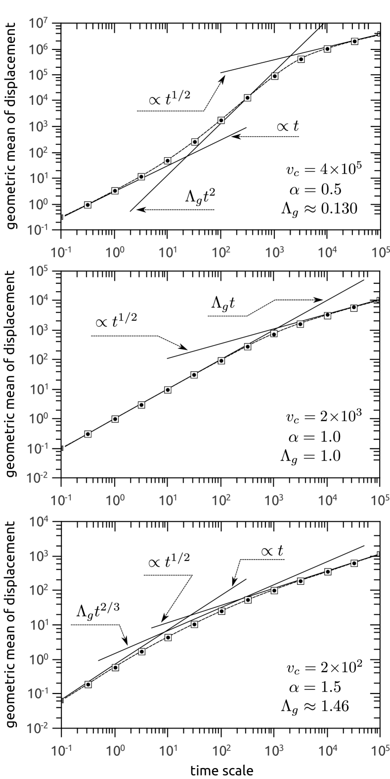
Figure 3: The geometric mean of the particle displacements vs the duration of time steps in the partitioning of the random walks. The symbols $\Box$ and • depict the data points for cases I and II, respectively.

Figure 3 visualizes the time dependence of the geometric mean $\overline{x}_{g}(t)$ for several values of the parameter $\alpha$, namely, $\alpha=0.5$, 1.0, and 1.5. These values match the superballistic, quasiballistic, and superdiffusive type of the expected Lévy scaling law $\overline{x}_{g}(t)\propto t^{1/\alpha}$. The choice of the corresponding values of the cutoff velocity $v_{c}$ will be explained below.

Appealing to the data plotted in Fig. 3 we can single out three characteristic stages in the $\overline{x}_{g}(t)$-dependence. First, on small scales the time dependence $\overline{x}_{g}(t)$ is found to be linear, as it must because of the strong velocity correlations for $t\lesssim 1$. Second, there is a certain intermediate stage that can be classified as the region of the Lévy scaling law. In fact, according to Ref. me3 random walks governed by model (9) with $v_{c}=\infty$ exhibit the Lévy type scaling law (18), i.e., $\overline{x}^{L}_{g}(t)=\Lambda_{g}t^{1/\alpha}$, when the duration of the trajectory partitioning fragments exceeds a certain value about 100, i.e., $t\gtrsim 100$ (in dimensionless units). So to make the intermediate Lévy asymptotics feasible, in the numerical simulation the critical velocity $v_{c}$ was chosen to exceed the geometric mean $\overline{x}_{g}(t)|_{t=100}$ for unlimited Lévy random walks tenfold. The employed values $v_{c}$ meeting this requirement are noted in Fig. 3. In order to clarify the fact that in the cases under consideration the geometric mean $\overline{x}_{g}(t)$ does exhibit the intermediate Lévy asymptotics the function $\Lambda_{g}t^{1/\alpha}$ is also plotted in Fig. 3. The lines visualizing this function are seen to be practically tangents to the curves interpolating the numerical data. Finally, for large values of time scale the cutoff effect becomes substantial and, as it must, the region of the classical asymptotics $\overline{x}_{g}(t)\propto t^{1/2}$ of Brownian motion arises.

It should be pointed out that in both cases I and II actually the same geometric mean $\overline{x}_{g}$ was obtained, which again justifies the previously drawn conclusion about the weak dependence of the given truncated Lévy random walks on the individual details of the kinetic coefficients $k(v)$ and $g(v)$.

4 Conclusion

The paper is devote to the development of a continuous theory of Lévy random walks that was recently initiated in Refs. me1 ; me2 ; me3 . Namely, a continuous Markovian model for truncated Lévy random walks has been developed. It is based on the nonlinear stochastic differential equation (9) governing the velocity $v$ of a wondering particle. The cutoff effects in the distribution of the particle velocity and displacement during a certain time interval can be caused by the velocity dependence of the friction coefficient as well as the saturation in the growth of the Langevin force intensity with the particle velocity. Both the mechanisms are studied individually and to be able to compare them against each other the system parameters have been chosen in such a manner that the velocity distribution be the same in both the cases. The one-dimensional system was analyzed numerically employing a strong stochastic Runge-Kutta methor of the stochastic order 1.5 Roussler . The obtained numerical data were used to calculate the geometric mean $\overline{x}_{g}(t)$ of the particle displacement $\delta_{t}x$ during the time interval $t$ and the probability density function $P(\rho,t)$ of this displacement normalized to its geometric mean, $\rho=\delta_{t}x/\overline{x}_{g}(t)$.

It has been demonstrated that the two mechanisms do give rise to truncated Lévy random walks on time scales exceeding substantially the “microscopic” time characterizing strong correlations in the velocity fluctuations. It is the case when the region $v\gtrsim v_{c}$, wherein the friction coefficient nonlinearity as well as the noise intensity saturation become substantial, is rather distant from the origin in the velocity space. As far as particular results are concerned, the following should be noted.

First, the time dependence of the geometric mean $\overline{x}_{g}(t)$ has been found to contain three characteristic asymptotics following one another as the time scale $t$ grows. The initial one matching the ballistic regime $\overline{x}_{g}(t)\propto t$ takes place for $t\lesssim 1$. The intermediate Lévy scaling law $\overline{x}_{g}(t)\propto t^{1/\alpha}$, which can represent the superballistic, quasiballistic, or superdiffusive regimes depending on the parameter $\alpha\in(0,2)$, is implemented for the time scales $t\gtrsim 100$. On larger scales the cutoff effects become substantial and the $\overline{x}_{g}(t)$-dependence converts into the classical law of Brownian motion, $\overline{x}_{g}(t)\propto t^{1/2}$.

Second, in the region of the Lévy scaling law the constructed probability density of the particle displacement $\delta_{t}x$ has been shown to be of the generalized Cauchy form with an exponential cutoff pronounced in the region $\delta_{t}x\gtrsim\Delta_{c}$. Using the numerical data the relationship $\Delta_{c}\sim v_{c}$ between the cutoff scale in the space of particle displacement and the velocity $v_{c}$ characterizing the nonlinearity of the kinetic coefficients is justified.

Finally, the properties of the given truncated Lévy random walks have turned out to depend weakly on the individual characteristics of the friction coefficient $k(v)$ and the noise intensity $g(v)$. Only the ratio $k(v)/g^{2}(v)$ specifying directly the stationary distribution of the particle velocity matters to them.

References

- (1) B. Mandelbrot, The Fractal Geometry of Nature (Freeman, San Francisco, 1982).
- (2) J.-P. Bouchaud and A. Georges, Phys. Rep. 195, 127 (1990).
- (3) B. J. West and W. Deering, Phys. Rep. 246, 1 (1994).
- (4) Lévy Flights and Related Topics in Physics, edited by M. F. Shlesinger, G. M. Zaslavsky, and U. Frisch (Springer, Berlin, 1995).
- (5) R. Metzler and J. Klafter, Phys. Rep. 339, 1 (2000).
- (6) Anomalous Transport, edited by R. Klages, G, Radons, and I. M. Sokolov (WILEY-VCH Verlag, Weinheim, 2008).
- (7) G. M. Viswanathan, E. P. Raposo, and M. G. E. da Luz, Phys. Life Rev. 5, 133 (2008).
- (8) A. M. Reynolds, J. Phys. A 42, 434006 (2009).
- (9) M. F. Shlesinger, J. Klafter, and Y. M. Wong, J. Stat. Phys. 27, 499 (1982).
- (10) M. F. Shlesinger, B. J. West, and J. Klafter, Phys. Rev. Lett. 58, 1100 (1987).
- (11) J. Klafter, A. Blumen, and M. F. Shlesinger, Phys. Rev. A 35, 3081 (1987);
- (12) R. N. Mantegna and H. E. Stanley, Phys. Rev. Lett. 73, 2946 (1994).
- (13) I. Koponen, Phys. Rev. E 52, 1197 (1995).
- (14) A. V. Chechkin, J. Klafter, V. Yu. Gonchar, R. Metzler, L. V. Tanatarov, Phys. Rev. E 67, 010102͑R͒ (2003).
- (15) A. V. Chechkin, V. Yu. Gonchar, J. Klafter, and R. Metzler, Phys. Rev. E 72, 010101(R) (2005).
- (16) I. Lubashevsky, R. Friedrich, and A. Heuer, Phys. Rev. E 79, 011110 (2009).
- (17) I. Lubashevsky, R. Friedrich, and A. Heuer, Phys. Rev. E 80, 031148 (2009).
- (18) I. Lubashevsky, A. Heuer, R. Friedrich, and R. Usmanov, Eur. Phys. J. B 78, 207 (2010).
- (19) H. Konno and F. Watanabe, J. Math. Phys. 48, 103303 (2007).
- (20) A. Schenzle and H. Brand, Phys. Rev. A 20, 1628 (1979).
- (21) S. C. Venkataramani, T. M. Antonsen Jr., E. Ott, and J. C. Sommerer, Physica D 96, 66 (1996).
- (22) H. Takayasu, A-H. Sato, and M. Takayasu, Phys. Rev. Lett. 79, 966 (1997).
- (23) J. M. Deutsch, Physica A 208, 433 (1994).
- (24) H. Sakaguchi, J. Phys. Soc. Japan, 70, 3247 (2001).
- (25) S. C. Lim and M. Li, J. Phys. A: Math. Gen. 39 2935 (2006).
- (26) T. Gneiting and M. Schlather, SIAM Rev. 46, 269 (2004).
- (27) H. Konno and Y. Tamura, Rep. Math. Phys. (2011) (to be published).
- (28) Yu. L. Klimontovich, Statistical Theory of Open Systems (Kluwer, Dordrecht, 1995).
- (29) B. Lindner, J. Stat. Phys. 130, 523 (2008).
- (30) S. Benhamou, Ecology 88, 1962 (2007).
- (31) A. Reynolds, Ecology 89, 2347 (2008).
- (32) S. Benhamou, Ecology 89, 2351 (2008).
- (33) A. Rößler, SIAM J. Numer. Anal. 48, 922 (2010).
- (34) M. Matsumoto and T. Nishimura, ACM Trans. Model. Comp. Simul. 8, 3 (1998).
- (35) URL: http://www.gnu.org/software/gsl/