Effects of Long-Range Correlations on Nonmagnetic Mott Transitions in Hubbard model on Square Lattice

Abstract

The mechanism of Mott transition in the Hubbard model on the square lattice is studied without explicit introduction of magnetic and superconducting correlations, using a variational Monte Carlo method. In the trial wave functions, we consider various types of binding factors between a doubly-occupied site (doublon, D) and an empty site (holon, H), like a long-range type as well as a conventional nearest-neighbor type, and add independent long-range D-D (H-H) factors. It is found that a wide choice of D-H binding factor leads to Mott transitions at critical values near the band width. We renew the D-H binding picture of Mott transitions by introducing two characteristic length scales, the D-H binding length $\ell_{\rm DH}$ and the minimum D-D distance $\ell_{\rm DD}$, which we appropriately estimate. A Mott transition takes place at $\ell_{\rm DH}=\ell_{\rm DD}$. In the metallic regime ($\ell_{\rm DH}>\ell_{\rm DD}$), the domains of D-H pairs overlap with one another, thereby doublons and holons can move independently by exchanging the partners one after another. In contrast, the D-D factors give only a minor contribution to the Mott transition.

1 Introduction

The Mott transitions[1] free from the spin degree of freedom were recently realized in ultracold bosonic atoms on optical lattices[2, 3, 4, 5]. In the Bose Hubbard models,[6] which faithfully describe these systems,[7, 8] superfluid-insulator (Mott) transitions occur when kinetic and interaction energies are competitive.[9, 10, 11, 12, 13, 14, 15, 16] It follows that the essence of “Mott physics” can be separated from magnetic metal-insulator transitions,[17] often arising in weakly correlated regimes in half-filled-band electronic systems, especially, with good nesting conditions. Aside from the spinless bosons, systems like organic superconductors $\kappa$-(BEDT-TTF) salts[18] and the cuprate superconductors as doped Mott insulators[19, 20, 21] require a deep understanding about the mechanism of nonmagnetic Mott transitions. Thus, it is significant to shed light on the Mott transition between virtual paramagnetic phases in the Hubbard model on the square lattice, which, though, actually has an antiferromagnetic (AF) long-range order for any finite value of positive $U/t$ ($U$: onsite correlation strength; $t$: hopping integral).[22, 23]

The variation theory[24, 25] has long been one of the main streams to study ground-state properties of the Mott transition. In particular, the variational Monte Carlo (VMC) approaches[26, 27, 28] are effective for its reliability in dealing with the local correlation and wide applicability. In the previous VMC studies related to paramagnetic Mott transitions, the following properties have been clarified. (i) The well-known Gutzwiller wave function,[24] with only onsite correlation, does not undergo a Mott transition for finite $U/t$ and in finite dimensions. Namely, the Brinkman-Rice transition[29, 25] is unreal.[28, 30] (ii) Wave functions with short-range intersite attractive correlations between a doubly-occupied site (doublon, D) and an empty site (holon, H)[31, 32, 33], which are minus and plus carriers in the neutral background (singly occupied sites), can properly describe the Mott transition.[34, 35, 36, 37] In particular in ref. YOT, the D-H binding-unbinding mechanism is studied for a projected $d$-wave singlet state as well as a projected Fermi sea for the two-dimensional Hubbard model ($t$-$t^{\prime}$-$U$ model). A similar result was also reached using a Jastrow-type wave function.[38] Later, we have found in two dimensions that Mott transitions occur even in the wave functions in which a doublon must be necessarily accompanied by at least one holon in the nearest-neighbor (NN) sites. Namely, the state in which a doublon and a holon always tightly bind one another can be metallic (see §4.1). This finding requires a modification of the above picture[37] of Mott transitions through D-H binding and a simple release from it.

In this paper, we address the following subjects by applying a VMC method to the half-filled-band Hubbard model on the square lattice: (i) We extend the D-H attractive correlation factors so as to include some long-range types, and corroborate the decisive effect of D-H binding on nonmagnetic metal-insulator transitions. (ii) We introduce long-range D-D (and H-H) factors independently of the above D-H factors. Thereby, we can distinguish the roles of the two factors for the Mott transition. (iii) We generalize the picture of the Mott transition so as to comprehend the one arising in the completely D-H bound state, and to treat it more quantitatively. By checking various wave functions, we are convinced that this conception is applicable to a wide range of systems, including Bose Hubbard models.[39]

This paper is organized as follows: In §2, the method used in this paper is formulated. In §3, we discuss various aspects of the VMC results. In §4, we propose an improved picture of Mott transitions, and confirm its applicability. Section 5 is assigned to summary.

A part of the results in this study was published before.[40]

2 Formulation

After brief introduction of the Hubbard model in §2.1, in §2.2, we describe the trial wave functions treated in this paper. In §2.3, we outline the VMC calculations.

2.1 Hubbard model on square lattice

We study the single-band Hubbard model with $t,U\geqq 0$,[24, 41, 42] which is fundamental to describe the physics of Mott transitions:[43]

$$H = H_{t}+H_{U}$$ (1)

$$= -t\sum_{\langle i,j\rangle,\sigma}{(c_{i\sigma}^{\dagger}c_{j\sigma}+c_{j\sigma}^{\dagger}c_{i\sigma})}+U\sum_{i}d_{i},\qquad$$

where $c_{i\sigma}$ is an electron annihilation operator of site $i$ and spin $\sigma$, $d_{i}=n_{i\uparrow}n_{i\downarrow}$ and $n_{i\sigma}=c_{i\sigma}^{\dagger}c_{i\sigma}$. In this paper, we focus on the case of half filling on the square lattice with only the nearest neighbor (NN) hopping,

$$H_{t} = \sum_{k}\epsilon_{k}c_{k\sigma}^{\dagger}c_{k\sigma},$$ (2)

$$\epsilon_{k} = -2t(\cos k_{x}+\cos k_{y}),$$ (3)

and use $t$ as the energy unit. In applying a variational Monte Carlo (VMC) method to this model, we use finite-size systems of $L\times L$ ($=N_{\rm s}$) sites up to $L=18$ ($N_{\rm s}=324$) with the periodic and antiperiodic boundary conditions in $x$ and $y$ directions, respectively, to meet the closed-shell condition.

2.2 Variational wave functions

In §2.2.1, we explain the conventional NN D-H binding wave function and the completely D-H bound state as its limiting case. In §2.2.2, we introduce a series of wave functions with long-range D-H binding factors and independent D-D (H-H) correlation factors.

2.2.1 Nearest-neighbor correlation factor

The simplest but fundamental trial wave function is the celebrated Gutzwiller wave function (GWF),[24]

$$\Psi_{\rm G}=P_{\rm G}\Phi_{\rm F},$$ (4)

where $\Phi_{\rm F}$ is the Fermi sea, and

$$P_{\rm G}=\prod_{j}\left[1-(1-g)d_{j}\right].$$ (5)

Here, $g$ is the variational parameter which adjusts the doublon density, $d=\sum_{j}\langle d_{j}\rangle/N_{\rm s}$. It is known that GWF is metallic for $U/t<\infty$.[28] To describe the Mott transition, a wave function[31, 33, 34] with a NN D-H binding correlation[44] has been often used:

$$\Psi_{\rm A(NN)}=P_{\rm A}^{\rm NN}\Psi_{\rm G}=\prod_{j}\left(1-\mu\hat{Q}_{j}\right)\Psi_{\rm G},$$ (6)

$$\hat{Q}_{j}=d_{j}\prod_{\vec{\tau}}(1-h_{j+\vec{\tau}})+h_{j}\prod_{\vec{\tau}}(1-d_{j+\vec{\tau}}),$$ (7)

where $h_{j}=(1-n_{j\uparrow})(1-n_{j\downarrow})$, $\mu$ ($0\leq\mu\leq 1$) is a variational parameter which controls the number of isolated doublons (D without H in its NN sites) and isolated holons, and $\vec{\tau}$ runs over the four NN sites of the site $j$. For $\mu=0$, $\Psi_{\rm A(NN)}$ is reduced to $\Psi_{\rm G}$. In the other limit, $\mu=1$, $\Psi_{\rm A(NN)}$ becomes the completely D-H bound state,

$$\Psi_{\rm A(bind)}=P_{\rm A}^{\rm bind}\Phi_{\rm G}=\prod_{j}\left\{1-\hat{Q}_{j}\right\}\Phi_{\rm G}.$$ (8)

In $\Psi_{\rm A(bind)}$, a doublon (holon) must be accompanied by at least one holon (doublon) in its NN sites, so that, superficially, $\Psi_{\rm A(bind)}$ always seems insulating. However, it turns out to be metallic for small $U/t$, because a doublon (holon) can have multiple holons (doublons) in its NN sites, as will be discussed in §4.1.

2.2.2 Long-range Jastrow factors

According to the result of exact diagonalization in the one-dimensional half-filled-band Hubbard model,[33] the ground state of which is a paramagnetic insulator for any positive $U/t$,[45] the magnitude of the coefficient of the basis having only one D-H pair with the D-H distance $r$ decreases exponentially with $r$ for large $U/t$. Assuming a similar situation arises in two dimensions, we introduce several types of long-range D-H attractive (A) correlation factors $P_{\rm A}$, and the corresponding D-D and H-H repulsive (R) factors $P_{\rm R}$:

$$P_{\rm A}=\prod_{j}\left(f_{\rm A}\left(|\vec{r}_{j}^{\rm A}|\right)\left\{d_{j}\left[1-\prod_{\vec{r}\in\{{\vec{r}_{j}^{\rm A}}\}}\left(1-h_{j+\vec{r}}\right)\right]\right.\right.$$

$$+\left.\left.h_{j}\left[1-\prod_{\vec{r}\in\{\vec{r}_{j}^{\rm A}\}}\left(1-d_{j+\vec{r}}\right)\right]\right\}\right),$$ (9)

$$P_{\rm R}=\prod_{j}\left(f_{\rm R}\left(|\vec{r}_{j}^{\rm R}|\right)\left\{d_{j}\left[1-\prod_{\vec{r}\in\{{\vec{r}_{j}^{\rm R}}\}}\left(1-d_{j+\vec{r}}\right)\right]\right.\right.$$

$$+\left.\left.h_{j}\left[1-\prod_{\vec{r}\in\{{\vec{r}_{j}^{\rm R}}\}}\left(1-h_{j+\vec{r}}\right)\right]\right\}\right),$$ (10)

where the index $j$ of the outer product runs over all the sites, and $\vec{r}_{j}^{\rm A}$ ($\vec{r}_{j}^{\rm R}$) indicates the vector from the site $j$ to the nearest partner. Namely, we disregard more distant ones, so that the index $\vec{r}$ of the products in eq. (9) runs over only the sites of the nearest D-to-H (in the first term) and H-to-D (in the second term) distances. This choice is reasonable in view of the strong-coupling expansion.[46] Correspondingly, we treat the product of $\vec{r}$ in eq. (10) in a similar way. To measure distances, we adopt the stepwise or Manhattan metric, in which, for instance, $r=2$ for $(i,j)\leftrightarrow(i+1,j+1)$, and the range is $1\leq r\leq L$. For each correlation, we consider the three forms:

$$f_{\rm A}(r)=\left\{\begin{array}[]{ll}\displaystyle\exp\left(-\frac{r-1}{\xi}\right),&\mbox{(a) exponential}\\ \displaystyle\frac{1}{r^{\xi}},&\mbox{(b) power law}\\ \displaystyle\xi_{r},&\mbox{(c) optimizing}\\ \end{array}\right.$$ (11)

$$f_{\rm R}(r)=\left\{\begin{array}[]{ll}\displaystyle 1-\alpha\exp\left(-\frac{r-1}{\beta}\right),&\mbox{(a) exponential}\\ \displaystyle 1-\frac{\alpha}{r^{\beta}},&\mbox{(b) power law}\\ \displaystyle\alpha_{r},&\mbox{(c) optimizing}\\ \end{array}\right.$$ (12)

where we fix $f_{\rm A}(1)$ and $f_{\rm R}(\infty)$ at unity for (a) and (b).

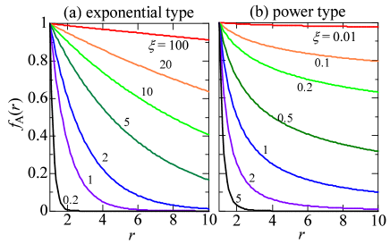
Figure 1: (Color online) Weight of long-range D-H attractive correlations as a function of distance between D and H; (a) an exponentially decaying type [eq. 11(a)], and (b) a power-law decaying type [eq. 11(b)].

In eq. (11), each $\xi$ ($\xi_{r}$) is a variational parameter. We consider two typical forms: (a) exponentially decaying and (b) power-law decaying, as shown in Fig. 1. Furthermore, in (c), we do not assume a specific form of $f_{\rm A}(r)$, and optimize all $\xi_{r}$’s ($2\leq r\leq L$) simultaneously as variational parameters. The type (c) is the best form of $f_{\rm A}(r)$, here; the other types are specific cases of (c). In eq. (12), we again assume the repulsive correlation becomes weaker, as $r$ increases. Corresponding to $f_{\rm A}(r)$, we consider three forms for $f_{\rm R}(r)$: (a) an exponentially and (b) a power-law decaying types, both with the parameters $\alpha$ adjusting the weight of $r=1$, and $\beta$ controlling the decaying length. In (c), we optimize all $\alpha_{r}$’s ($1\leq r\leq L$) simultaneously. Notice that here we permit $\alpha_{r}$ to be larger than 1, meaning $P_{\rm R}$ possibly works as D-D (H-H) attractive correlations.

Table 1: Summary of trial wave functions. In the second column, we abbreviate the type of correlation, with GW being the onsite (Gutzwiller) repulsion.

$\Psi$	correlation	correlation	param.
abbreviation	type	range	number
GWF	GW	onsite	1
A(NN)	GW+DH	NN	2
A(bind)	GW+DH	NN	1
A(exp)	GW+DH	long	2
R(exp)	GW+DD	long	3
AR(exp)	GW+DH+DD	long	4
A(pow)	GW+DH	long	2
R(pow)	GW+DD	long	3
AR(pow)	GW+DH+DD	long	4
A(opt)	GW+DH	long	$L$
R(opt)	GW+DD	long	$L$+1
AR(opt)	GW+DH+DD	long	2$L$

In this work, we study a series of wave functions by combining the above correlation factors as follows:

$$\begin{array}[]{l}\;\;\Psi_{\rm A(exp)}=P_{\rm A}^{\rm(a)}\Psi_{\rm G},\\ \;\;\Psi_{\rm R(exp)}=P_{\rm R}^{\rm(a)}\Psi_{\rm G},\\ \Psi_{\rm AR(exp)}=P_{\rm A}^{\rm(a)}P_{\rm R}^{\rm(a)}\Psi_{\rm G},\end{array}$$ (13)

$$\begin{array}[]{l}\;\;\Psi_{\rm A(pow)}=P_{\rm A}^{\rm(b)}\Psi_{\rm G},\\ \;\;\Psi_{\rm R(pow)}=P_{\rm R}^{\rm(b)}\Psi_{\rm G},\\ \Psi_{\rm AR(pow)}=P_{\rm A}^{\rm(b)}P_{\rm R}^{\rm(b)}\Psi_{\rm G},\end{array}$$ (14)

$$\begin{array}[]{l}\;\;\Psi_{\rm A(opt)}=P_{\rm A}^{\rm(c)}\Psi_{\rm G},\\ \;\;\Psi_{\rm R(opt)}=P_{\rm R}^{\rm(c)}\Psi_{\rm G},\\ \Psi_{\rm AR(opt)}=P_{\rm A}^{\rm(c)}P_{\rm R}^{\rm(c)}\Psi_{\rm G},\end{array}$$ (15)

where the superscripts of $P_{\rm A}$ and $P_{\rm R}$ correspond to the function types (a)-(c) in eqs. (11) and (12). For $\Psi_{\rm AR}$, we unify the function types of $f_{\rm A}(r)$ and $f_{\rm R}(r)$, for simplicity. In Table. 1, we summarize the used wave functions.

Note that the projector $P_{\rm A}^{\rm(c)}P_{\rm R}^{\rm(c)}$ in eq. (15) is different from the Jastrow factor used in related papers,[47, 38] especially in that the magnitude of long-range D-D factor in them is connected to the inverse of corresponding D-H attractive factor, so that the D-D factor is necessarily repulsive as far as the D-H factor is attractive.

2.3 Variational Monte Carlo calculations

In this subsection, we briefly describe the outline of VMC calculations implemented in this study.

A correlated measurement or optimization-VMC technique[48] is used to optimize variational parameters up to $2L$. In the non-linear minimization process of energy expectation values for the wave functions with many parameters, we adopt a quasi-Newton method, in which gradient vectors are effectively calculated by recently proposed formulae,[49] and Hessian matrices are approximated by Broyden-Flecher-Goldfarb-Shanno formula,[50] the use of which does not affect the exactness of optimization itself. In coding, we refer to an algorithm offered by Ibaraki and Fukushima.[51] For wave functions with a few parameters, we use a simple linear optimization together.

In both algorithms, parameters as well as energy converge typically after first several rounds of iteration with different fixed sample sets; in each set we generate typically $2.5\times 10^{5}$ particle configurations using Metropolis algorithm. After the convergence, we continue excess rounds (10-20 times) of iteration in the optimization process with successively renewed configuration sets. We determine the optimized values by averaging the data obtained in the excess rounds; in averaging, we exclude scattered data beyond the range of twice the standard deviation. The optimal value is an average of substantially more than several million samples. The variational energy and significant parameters [$g$, $\mu$, $\xi$, etc.] are obtained with sufficient accuracy, but the determination of insignificant parameters [$f_{\rm A}(r)$ and $f_{\rm R}(r)$ with $r>8$, etc.] is difficult, because $E$ depends on them only very slightly, in other words, particle configurations determining them appear extremely rarely. Anyway, such parameters have little influence on $E$ and other quantities. Physical quantities are calculated typically with $2.5\times 10^{5}$ renewed configurations generated by the optimized parameter sets.

Since in Mott critical regimes, the global minimum becomes more competitive with other local minima as $L$ increases, accurate energy minimization sometimes becomes not easy. This leads to the scattered data points near $U_{c}/t$ in some figures.

3 Results

In this section, we discuss the results of VMC calculations. In §3.1 and §3.2, energies and other quantities obtained by various wave functions are studied, respectively, in view of the Mott transition. In §3.3, the system-size dependence of the Mott critical values are discussed. In §3.4, the differences among various D-H factors are studied. In §3.5, we discuss the effects of repulsive long-range factors.

3.1 Behavior of energy

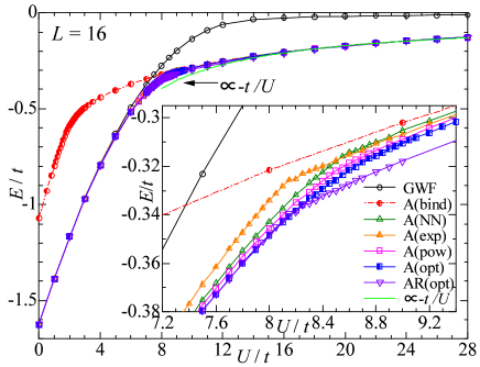
Figure 2: (Color online) Comparison of variational energies among various trial wave functions as function of correlation strength for $L=16$. The pale solid line is a guide line proportional to $-t/U$ expected from the strong-coupling expansion. The inset shows a magnification near the crossing point of GWF and A(bind).

First of all, let us discuss the behavior of total energy per site $E/t$. In the main panel of Fig. 2, we compare $E/t$ among various wave functions in a wide range of $U/t$. Here, we notice GWF and the completely bound state $\Psi_{\rm A(bind)}$. It is known that GWF is metallic for $U/t<\infty$ and a relatively good for $U$ sufficiently smaller than the critical value of the Brinkman-Rice transition, $U_{\rm BR}=12.97t$.[25] On the other hand, $\Psi_{\rm A(bind)}$ is insulating for $U/t\ \raise 1.50696pt\hbox{$>$}\kern-7.5pt\lower 2.15277pt\hbox{$\sim$}\ 3$ (see §4.1), which fact is supported by the coincidence with the result of strong coupling expansion $\propto-t/U$,[46] as shown in Fig. 2. $E/t$ of GWF is much lower than that of $\Psi_{\rm A(bind)}$ for $U/t<7.4$, while the relation is reversed for $U/t>7.4$, suggesting the phase switches from metal to insulator at $U/t\sim 7.4$. Now, we look at the D-H binding wave functions ($\Psi_{\rm A}$). $E/t$ of all $\Psi_{\rm A}$’s [$E({\rm A})$] except for $\Psi_{\rm A(bind)}$ behave similarly, namely, $E({\rm A})$ is very close to $E({\rm GWF})$ for $U/t\ \raise 1.50696pt\hbox{$<$}\kern-7.5pt\lower 2.15277pt\hbox{$\sim$}\ 5$, somewhat smaller than both $E({\rm GWF})$ and $E(\Psi_{\rm A(bind)})$ for the intermediate values of $U/t$, and approaches $E(\Psi_{\rm A(bind)})$ for $U/t\ \raise 1.50696pt\hbox{$>$}\kern-7.5pt\lower 2.15277pt\hbox{$\sim$}\ 9$. Hence, a wide class of D-H binding wave functions probably induces Mott transitions at $U\sim W$ [$W(=8t)$: band width]. This is consistent with the previous result for a short-range D-H binding wave function, in which a first-order Mott transition occur at $U_{\rm c}/t$=8.59 and 8.73 for $L=16$ and 18, respectively.[37]

The detailed behavior of $E({\rm A})$ for intermediate $U/t$ is different among different types of D-H factors, as shown in the inset of Fig. 2. For example, $E(\Psi_{\rm A(exp)})$ exhibits a clear cusp at $U\sim 8.12t$ $(\equiv U_{\rm c})$, and has a higher value than those of other $E({\rm A})$’s for $U<U_{\rm c}$, whereas $E(\Psi_{\rm A(opt)})$ exhibits smooth behavior in this regime, and has a lower value. The energy of the best function $\Psi_{\rm AR(opt)}$ is broadly similar to $E(\Psi_{\rm A(opt)})$ for $U\leq U_{\rm c}$, but has an appreciably lower energy for $U>U_{\rm c}$. We will return to this subject in §3.4.

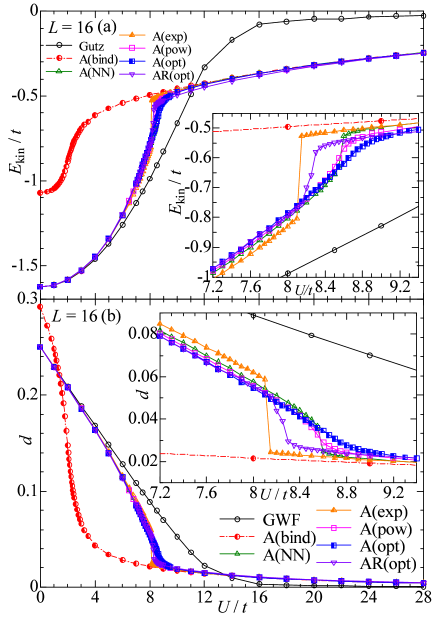
Figure 3: (Color online) The expectation values of (a) kinetic energy and (b) doublon density (interaction energy) are compared among the identical wave functions treated in Fig. 2. The insets show magnifications near the Mott critical points.

Next, we consider the components of energy. Although the total energy should be a continuous function of $U/t$, its components can exhibit stronger critical anomalies at $U_{\rm c}/t$ if the transition is first order. Figures 3(a) and 3(b) shows the kinetic energy, $E_{\rm kin}=\langle H_{t}\rangle/N_{\rm s}$, and doublon density (substantial interaction energy), $d=E_{\rm int}/U=\langle H_{U}\rangle/(UN_{\rm s})$, respectively. As evidently seen in the insets, $\Psi_{\rm A(exp)}$, which exhibits a clear cusp in $E/t$, has discontinuities at $U_{\rm c}/t$ in $E_{\rm kin}$ and $d$. This is an obvious sign of a first-order transition; actually we have observed a hysteresis around the critical point. Other wave functions behave more mildly at this system size, but the behavior evolves into more first-order-like as $L$ increases, as we will discuss in §3.3. The fact that $E_{\rm kin}$ ($d$) of every D-H binding wave function abruptly increases (decreases) in the critical region as $U/t$ increases is consistent with a requisite of the Mott transition: The metal-to-insulator transition is driven by reducing the interaction energy at the cost of the kinetic energy. This is in sharp contrast with antiferromagnetic and superconducting transitions arising in strongly correlated regimes.[35, 21]

3.2 Critical behavior of physical quantities

To corroborate the realization of Mott transition in $\Psi_{\rm A}$ and estimate the critical value more accurately, we consider other physical quantities.

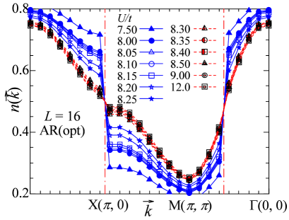
Figure 4: (Color online) The momentum distribution function is shown along the path, $(0,0)$$\rightarrow$$(\pi,0)$$\rightarrow$$(\pi,\pi)$$\rightarrow$$(0,0)$, calculated with the wave funcition AR(opt) for various values of $U/t$ near $U_{\rm c}/t\sim 8.27$ for $L=16$. The vertical dash-dotted lines indicate the positions of $\vec{k}_{\rm F}$ in the metallic cases.

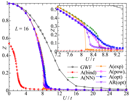
Figure 5: (Color online) Quasiparticle renormalization factor as function of $U/t$, estimated from discontinuities in $n(\vec{k})$ at $\vec{k}=(\pi,0)$ for various type of wave functions. The inset shows the magnification near the Mott critical points. A(bind) will be discussed later.

First, we discuss the momentum distribution function,

$$n(\vec{k})=\frac{1}{2}\sum_{\sigma}\langle c_{\vec{k}\sigma}^{\dagger}c_{\vec{k}\sigma}\rangle=\frac{1}{2N_{s}}\sum_{\vec{j},\vec{\ell},\sigma}e^{i\vec{k}\cdot\vec{\ell}}\left<c_{\vec{j}+\vec{\ell}\sigma}^{\dagger}c_{\vec{j}\sigma}\right>.$$ (16)

In Fig. 4, we show, as a typical case, the result of $\Psi_{\rm AR(opt)}$, which exhibits first-order-like critical behavior in energy at $U_{\rm c}/t\sim 8.30$ (Fig. 3). Let us pay attention to the behavior around the Fermi surface near $\vec{k}=(\pi,0)$. For small values of $U/t$ ($<8.3$), a discontinuity of $n(\vec{k})$ is evident at $\vec{k}_{\rm F}$, whereas the magnitude of discontinuity abruptly becomes small at $U\sim U_{\rm c}$ and remains very small for large $U/t$ ($>8.3$). To discuss quantitatively, we actually measure the jump of $n(\vec{k})$, namely quasiparticle renormalization factor $Z$, at the X point $(\pi,0)$:

$$Z=n^{-}(k)|_{k\rightarrow X-0}-n^{+}(k)|_{k\rightarrow X+0},$$ (17)

where $n^{-}(k)$ [$n^{+}(k)$] is the fitting function of the segment $\Gamma$-X [X-M] of $n(\vec{k})$ given by the third-order of least squares method. According to the Fermi liquid theory, $Z$ becomes zero for insulating states. As shown in Fig. 5, $Z$ of every D-H binding function almost vanishes at $U/t=8.2$-9.0, although the detailed behavior somewhat differs among different wave functions. The small residual values for large $U/t$ are owing to the finite system sizes. Thus, we may regard the states for $U/t\ \raise 1.50696pt\hbox{$>$}\kern-7.5pt\lower 2.15277pt\hbox{$\sim$}\ 9$ as insulating. As for $\Psi_{\rm AR(opt)}$, $Z$ most markedly drops at 8.2-8.3, which coincides with $U_{\rm c}/t$ evaluated from energy. In contrast, $Z$ of a metallic state GWF asymptotically approaches zero, as known.[34]

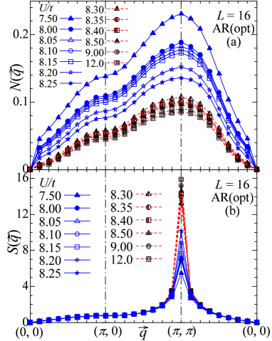
Figure 6: (Color online) (a) Charge density structure factor of AR(opt) for some values of $U/t$ near $U_{\rm c}/t\sim 8.3$. (b) Spin structure factor of AR(opt) for the same condition as (a).

Second, we consider the charge density correlation function in the wave-number space,

$$N({\vec{q}})=\frac{1}{N_{\rm s}}\sum_{i,j}e^{i{\vec{q}}\cdot({\vec{r}}_{i}-{\vec{r}}_{j})}\left\langle{n_{i}n_{j}}\right\rangle-n^{2},$$ (18)

which is known, within the variation theory, to behave as $N(\vec{q})\propto|\vec{q}|$ for $|\vec{q}|\rightarrow 0$ unless an excitation gap opens in the charge degree of freedom, whereas $N(\vec{q})\propto|\vec{q}|^{2}$ if a charge gap opens. Figure 6(a) shows $N(\vec{q})$ of $\Psi_{\rm AR(opt)}$; the behavior for small values of $|\vec{q}|$ abruptly changes between $U/t=8.25$ and 8.3, which again coincide with $U_{\rm c}/t$ determined by other quantities. For $U>U_{\rm c}$, the behavior becomes $|\vec{q}|^{2}$-like, suggesting a charge gap opens.

Third, we study the spin correlation function,

$$S({\vec{q}})=\frac{1}{N_{\rm s}}\sum_{ij}{e^{i{\vec{q}}\cdot({\vec{r}}_{i}-{\vec{r}}_{j})}\left\langle{S_{i}^{z}S_{j}^{z}}\right\rangle}.$$ (19)

In Fig. 6(b), $S({\vec{q}})$ of $\Psi_{\rm AR(opt)}$ is plotted for the same range of $U/t$ as in (a). For small $|\vec{q}|$, the behavior is always $S({\vec{q}})\propto|q|$, suggesting the low-lying spin excitation is gapless both in metallic and insulating phases. On the other hand, the magnitude at the AF nesting vector $\vec{q}=(\pi,\pi)$ increases as $U/t$ increases, in particular, markedly at $U/t=8.3$. Thus, the D-H binding wave function shows strong inclination toward the antiferromagnetic order, especially in the insulating case. This aspect is the same as the short-range D-H binding wave functions.[37]

3.3 System-size dependence of critical point

In this subsection, we consider the system-size dependence of the Mott critical point, which we have disregarded to this point.

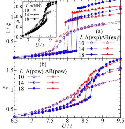
Figure 7: (Color online) The behavior of optimized variational parameters which controls D-H binding strength is compared among three system sizes near the Mott critical points. The results for three types of wave functions are shown: (a) $1/\xi$ for A(exp) and AR(exp). The inset shows $\mu$ for A(NN). (b) $\xi$ for A(pow) and AR(pow).

The optimized variational parameters controlling the D-H binding strength is important to definitely determine the critical values. In the main panel of Fig 7(a), the optimized $1/\xi$ in the wave functions of the exponentially-decaying type [eq. (11a)] is plotted for three system sizes. For small systems like $L=10$, the variation of $1/\xi$ is smooth and clear critical behavior is not seen, whereas systems with $L\geq 14$ exhibit clear discontinuities. Such tendency is often observed when finite systems are used,[52] because the phase transition is well defined for $L=\infty$. As another example, we show the result for the short-range D-H correlation in the inset of Fig. 7(a).[37, 39]

It is also a general tendency of the D-H binding wave functions that the Mott critical value increases as $L$ increases.[37, 39] This stems from the great system-size dependence in $E/t$ in the insulating side of the transition point, compared with in the metallic side. This is reflected in some decrease of the critical value by adding repulsive Jastrow factors [$\Psi_{\rm AR(exp)}$], which improve $E/t$ especially in the insulating side, as in the inset of Fig. 2.

Table 2: The Mott critical values, $U_{\rm c}/t$, estimated from eq. (20) is entered in the first line of each wave function. The results of five system sizes are compared. The figures in the second line represent the critical values determined by the crossing point of $\ell_{\rm DH}$ and $\ell_{\rm DD}$, which will be discussed in §4. The figures with * for A(bind) are estimated from $Z$, which will be explained in §4.1.

$\Psi$	$L=10$	$L=12$	$L=14$	$L=16$	$L=18$
A(NN)	7.85	8.25	8.475	8.575	8.675
$\ell_{\rm DH}=\ell_{\rm DD}$	8.85	8.725	8.575	8.575	8.875
A(exp)	7.75	7.875	8.025	8.125	8.275
$\ell_{\rm DH}=\ell_{\rm DD}$	7.95	7.875	8.025	8.125	8.275
AR(exp)	7.65	7.775	7.925	8.025	8.125
$\ell_{\rm DH}=\ell_{\rm DD}$	7.75	7.775	7.925	8.025	8.125
A(pow)	7.55	7.95	8.375	8.575	8.675
$\ell_{\rm DH}=\ell_{\rm DD}$	8.55	8.475	8.525	8.625	8.725
AR(pow)	7.65	7.95	8.175	8.375	8.525
$\ell_{\rm DH}=\ell_{\rm DD}$	8.35	8.275	8.325	8.425	8.525
A(opt)	7.15	8.075	8.275	8.525	8.875
$\ell_{\rm DH}=\ell_{\rm DD}$	8.75	8.775	8.825	8.925	9.025
AR(opt)	7.45	7.925	8.125	8.275	8.375
$\ell_{\rm DH}=\ell_{\rm DD}$	8.225	8.125	8.175	8.275	8.375
A(bind)	2.10*	2.28*	2.365*	2.39*	2.42*
$\ell^{*}_{\rm DD}=3$	2.00	2.175	2.275	2.375	2.425

These tendencies are common to other D-H binding wave functions; as another example, in Fig. 7(b), we show optimized $\xi$ in the power-law decaying correlation factor eq. (11b). In $\Psi_{\rm A(pow)}$, the critical behavior is less clear. In case the Mott critical point cannot be clearly determined, we estimate $U_{\rm c}/t$ from the maximum of the decreasing rate of doublon density $d$,

$$-\frac{\partial d}{\partial(U/t)}=-\frac{d[(U+\Delta U)/t]-d[U/t]}{\Delta U/t}.$$ (20)

The Mott critical values thus obtained are summarized in Table 2.

3.4 Effects of different D-H binding factors

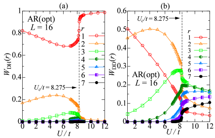
Figure 8: (Color online) The appearance rates of nearest (a) D-H and (b) D-D distances of $r$ are plotted for $r=1$-7 as a function of $U/t$. Both $W_{\rm DH}$ and $W_{\rm DD}$ are calculated with AR(opt). The vertical dashed lines indicate the Mott critical point.

First of all, we look at the distribution of distance from a doublon (holon) to the nearest holon (doublon), which is denoted simply by $r$, here. We indicate the appearance rate of $r$ by $W_{\rm DH}(r)$, which satisfies,

$$\sum_{r=1}^{L}W_{\rm DH}(r)=1.$$ (21)

In Fig. 8(a), $W_{\rm DH}(r)$ with $r\leq 7$ for the best function $\Psi_{\rm AR(opt)}$ is depicted versus $U/t$. In the metallic regime, $W_{\rm DH}(1)$ is predominant, but $W_{\rm DH}(r)$ with $r\geq 2$ has an appreciable weight especially at $U/t\sim 6$; there, a doublon is detached from holons to some extent. Meanwhile, in the insulating regime, the weight is almost concentrated on $r=1$, indicating D-H pairs are confined within mutually NN sites. In a similar way, we define $W_{\rm DD}(r)$ as the appearance rate of doublons (holons) with the D-to-D (H-to-H) distance of $r$. As shown in Fig. 8(b), $W_{\rm DD}(r)$ of large $r$ increases and $W_{\rm DD}(1)$ and $W_{\rm DD}(2)$ rapidly decreases, as $U/t$ increases. In the insulating phase, doublons tend to keep away from each other.

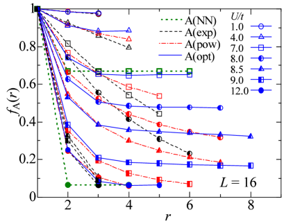
Figure 9: (Color online) Comparison of optimized D-H attractive correlation weight $f_{\rm A}(r)$ among four D-H binding wave functions, A(NN), A(exp), A(pow) and A(opt), for various values of $U/t$. We omit the data which do not meet the condition (22).

In the following, we discuss the effects of different D-H binding factors $P_{\rm A}^{({\rm x})}$ (x = a, b, c, NN), without introducing repulsive correlations. Figure 9 compares the optimized weights $f_{\rm A}(r)$ [eq. (11)] among the four D-H projectors. The plotted data are restricted to what satisfies the following condition:

$$\rho(r)>\rho_{\rm min},$$ (22)

where $r$ has the same meaning as in the preceding paragraph, and $\rho(r)$ [$=W_{\rm DH}(r)\times d$ ] denotes the appearance probability of the doublon (holon) of $r$. After a search, we put $\rho_{\rm min}=4\times 10^{-4}$, which corresponds to the probability that doublons or holons of certain $r$ appear $10^{4}$ times in $2.5\times 10^{5}$ samples for the system of $L=10$. If the condition (22) is not satisfied for $r=r^{*}$, the optimized $f_{\rm A}(r^{*})$ become statistically unreliable in the present calculations, and corresponding samples actually make only an imperceptible contribution to the averages.

We start with the analysis of the optimizing-type wave function $\Psi_{\rm A(opt)}$. For any values of $U/t$, $f_{\rm A}(r)$ rapidly decreases for $r\ \raise 1.50696pt\hbox{$<$}\kern-7.5pt\lower 2.15277pt\hbox{$\sim$}\ 3$, but becomes almost constant for $r\ \raise 1.50696pt\hbox{$>$}\kern-7.5pt\lower 2.15277pt\hbox{$\sim$}\ 3$. Note that this long-range behavior of $f_{\rm A}(r)$ is convenient for the conductive nature in the metallic regime ($U<U_{\rm c}$), namely, a doublon is released from the bondage of holons, once a doublon goes three lattice constants away from holons. The effective range of $f_{\rm A}(r)$ satisfying the condition (22) becomes the widest ($r\ \raise 1.50696pt\hbox{$<$}\kern-7.5pt\lower 2.15277pt\hbox{$\sim$}\ 8$) near $U_{\rm c}/t$, but abruptly shrinks in the insulating phase, as expected from the data in Fig. 8(a). In addition, for $U>U_{\rm c}$, the magnitude of $f_{\rm A}(r)$ itself is small. As a result, a doublon and a holon come to confine each other in a narrow D-H pair domain. We will return to this topic as to the mechanism of Mott transitions in §4. The propriety of other $\Psi_{\rm A}$ depends on how properly $f_{\rm A}(r)$ of $\Psi_{\rm A}$ can imitate that of $\Psi_{\rm A(opt)}$.

Regarding a short-range D-H factor, the reason why simple $\Psi_{\rm A(NN)}$ is unexpectedly good for $U<U_{\rm c}$ (inset of Fig. 2) is that $f_{\rm A}(r)$ of $\Psi_{\rm A(NN)}$ is constant for $r\geq 2$ and resembles that of $\Psi_{\rm A(opt)}$ except for $f_{\rm A}(2)$, as shown in Fig. 9 for the data of $U/t=7$. On the other hand, the reason why $E/t$ of $\Psi_{\rm A(NN)}$ is relatively high in the insulating regime, as compared with the other $\Psi_{\rm A}$, stems from an underestimate of $f_{\rm A}(2)$, as seen for $U/t=12$.

We turn to the long-range D-H factors. In the metallic regime, $f_{\rm A}(r)$’s of $\Psi_{\rm A(pow)}$ and especially of $\Psi_{\rm A(exp)}$ are underestimated for small $r$ and overestimated for large $r$, to be optimized as a whole. Consequently, $\Psi_{\rm A(exp)}$ has appreciably higher energy than other $\Psi_{\rm A}$’s; this behavior lowers the Mott critical value of $\Psi_{\rm A(exp)}$. On the other hand, in the insulating regime, $f_{\rm A}(r)$’s of both $\Psi_{\rm A(exp)}$ and $\Psi_{\rm A(pow)}$ almost coincide with that of $\Psi_{\rm A(opt)}$, because the long-range part of $f_{\rm A}(r)$ ($r\ \raise 1.50696pt\hbox{$>$}\kern-7.5pt\lower 2.15277pt\hbox{$\sim$}\ 3$) substantially vanishes. As a result, $E(\Psi_{\rm A(exp)})$ and $E(\Psi_{\rm A(pow)})$ become as good as $E(\Psi_{\rm A(opt)})$.

3.5 Effects of repulsive intersite correlations

First of all, we compare contributions to the improvement of energy between D-H attractive and D-D (and H-H) repulsive correlation factors. In Table 3, the optimized total energies of GWF and the optimizing-type wave functions eq. (15) are summarized. The results of other types of wave functions eqs. (13) and (14) are basically identical as far as the effect of repulsive factors is concerned. The wave function $\Psi_{\rm R(opt)}$ [eq. (15)], in which only the repulsive factor $P_{\rm R}$ [eq. (10) with eq. (12c)] is applied to GWF, improves $E/t$ only very slightly on GWF for any value of $U/t$. Furthermore, $\Psi_{\rm R(opt)}$ never induces a Mott transition, like GWF. Thus, the repulsive correlation $P_{\rm R}$, by itself, make no substantial improvement on GWF. In contrast, as already discussed for Table 2 and Fig. 2, $\Psi_{\rm A(opt)}$ induces a Mott transition, and make a great improvement in $E/t$ on GWF for $U\ \raise 1.50696pt\hbox{$>$}\kern-7.5pt\lower 2.15277pt\hbox{$\sim$}\ U_{\rm c}$, conclusively showing that the essence of Mott transition is included in the D-H binding correlation. $\Psi_{\rm AR(opt)}$ ($=P_{\rm R}\Psi_{\rm A(opt)}$) further reduces $E/t$ for $U>U_{\rm c}$. Although the decrement in energy thereby is as small as 2% of $E(\Psi_{\rm A(opt)})$ [$U/t=9$ and 12], the addition of $P_{\rm R}$ shifts the Mott critical point to a somewhat lower value (Table 2), and make the critical behavior more first-order-like (inset of Fig. 5).

Table 3: Comparison of variational energies $E/t$ among GWF and the optimizing type of wave functions, eq. (15), for $L=16$. The digits in the brackets denotes the error in the last digits.

$U/t$	GWF	R(opt)	A(opt)	AR(opt)
1.0	-1.3865(2)	-1.3866(3)	-1.3867(4)	-1.3867(3)
7.0	-0.374(1)	-0.375(2)	-0.418(2)	-0.418(2)
7.5	-0.323(2)	-0.323(2)	-0.379(2)	-0.379(2)
8.0	-0.276(2)	-0.277(2)	-0.348(2)	-0.348(3)
8.5	-0.234(2)	-0.234(2)	-0.325(3)	-0.330(2)
9.0	-0.196(2)	-0.197(2)	-0.310(2)	-0.317(2)
12.0	-0.061(2)	-0.063(2)	-0.255(3)	-0.261(2)

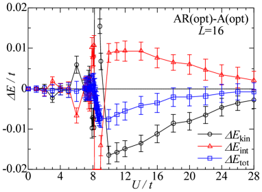
Figure 10: (Color online) The differences of total, kinetic and interaction energies between AR(opt) and A(opt) are plotted as a function of $U/t$ for $L=16$. If the value is negative, AR(opt) has a lower energy than A(R). The large deviations near $U_{\rm c}/t$ should be neglected, which stem from the discordance of $U_{\rm c}/t$.

Next, we consider the differences of kinetic and of interaction energies between $\Psi_{\rm AR(opt)}$ and $\Psi_{\rm A(opt)}$:

$$\Delta E_{\Gamma}=E_{\Gamma}[\mbox{AR(opt)}]-E_{\Gamma}[\mbox{A(opt)}]$$ (23)

where the suffix $\Gamma$ denotes “kin”, “int” or “tot”. In Fig .10, the three kinds of $\Delta E$ are plotted versus $U/t$. In the metallic regime, not only $\Delta E_{\rm tot}$ remains zero, but also both $\Delta E_{\rm kin}$ and $\Delta E_{\rm int}$ are zero except for irregular accidental deviations. Thus, $P_{\rm R}$ does not modify $E(\Psi_{\rm A(opt)})$ for $U<U_{\rm c}$. Nevertheless, for $U/t>10$ in the insulating regime, $\Delta E_{\rm kin}$ exhibits appreciable negative values, according to $\Delta E_{\rm tot}$. Inversely, $\Delta E_{\rm pot}$ has regular positive values; $P_{\rm R}$ with the aid of $P_{\rm A}$ reduces $E_{\rm kin}$ at the cost of $E_{\rm int}$ in the insulating phase. Thus, $P_{\rm R}$ compensates for the excess of D-H binding effects.

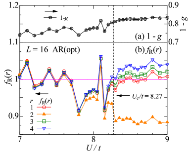
Figure 11: (Color online) (a) Optimized onsite repulsive (Gutzwiller) parameter $g$ near the Mott critical point. (b) Optimized long-range repulsive correlation weight $f_{\rm R}(r)$, eq. (12c). The results in (a) and (b) are obtained in an identical calculation for AR(exp).

Finally, we discuss the repulsive correlation weight for $\Psi_{\rm AR(opt)}$, in which $f_{\rm R}(r)$ is optimized for each $r$. In Fig. 11(b), $f_{\rm R}(r)$ for $r\leq 4$ is shown near $U_{\rm c}/t$. In the metallic regime, $f_{\rm R}(r)$ is almost unity, although there is some fluctuations, indicating the repulsive intersite correlation is virtually ineffective. Correspondingly, $\Psi_{\rm AR(opt)}$ seldom improves $E/t$ on that of $\Psi_{\rm A(opt)}$ for $U<U_{\rm c}$ (Table 3). Meanwhile, in the insulating regime, only $f_{\rm R}(2)$ is slightly lowered from unity, causing the sudden drop of $W_{\rm DD}(2)$ for $U>U_{\rm c}$ [Fig. 8(b)].[53] The behavior of $f_{\rm R}(r)>1$ for $r\geq 3$ indicates that D-D and H-H correlations are attractive rather than repulsive in a long-range part.[54] This behavior promotes the repulsion between doublons in proximity, as seen in Fig. 8(b), where $W_{\rm DD}(r)$ for $r>3$ is larger than $W_{\rm DD}(1)$. These effects of $f_{\rm R}(r)$ causes a small but steady improvement in energy on $\Psi_{\rm A(opt)}$ (Table 3). Incidentally, the scattered data, especially for $U<U_{\rm c}$, stem from the complementarity between the onsite and intersite repulsive correlations. The behavior of $g$ in Fig. 11(a) is quite opposite to that of $f_{\rm R}(r)$ in Fig. 11(b). Owing to the balance between the two, the resultant physical quantities become smooth, for instance, $d$ in Fig. 16. In this point, the parameter space has redundancy.

4 Improved Picture of Mott Transitions

In §4.1, we discuss the Mott transition arising in the completely D-H bound state, and provide a reformed picture of Mott transitions to comprehend it. In §4.2, we show that this picture is applicable to various D-H binding wave functions.

4.1 Mott transition in completely D-H bound state

In §3.1, we supposed that the completely D-H bound wave function $\Psi_{\rm A(bind)}$ [eq. (8)] represents a typical insulating state, but this supposition is not true for small values of $U/t$. The total energy of $\Psi_{\rm A(bind)}$ in Fig. 2 exhibits an abrupt change of curvature at $U/t\sim 2.5$. Corroboratively, as shown in Fig. 5, the quasiparticle renormalization factor $Z$ has finite values for $U/t\ \raise 1.50696pt\hbox{$<$}\kern-7.5pt\lower 2.15277pt\hbox{$\sim$}\ 2.5$. Thus, it is certain that $\Psi_{\rm A(bind)}$ exhibits a Mott transition and is metallic for small $U/t$. Then, we estimate the Mott critical values of $\Psi_{\rm A(bind)}$ from the extrapolation of $Z$ for $U/t\ \raise 1.50696pt\hbox{$<$}\kern-7.5pt\lower 2.15277pt\hbox{$\sim$}\ 2$ using the third-order least squares method, as shown in Fig. 12, and summarize them in Table 2. In $\Psi_{\rm A(bind)}$, doublons (holons) must be accompanied by at least one holon (doublon) in its NN sites. The metallic state satisfying this condition cannot be represented simply by the unbinding of D-H pairs proposed in ref. YOT. In what follows, we consider a microscopic picture of Mott transitions which comprehends the case of $\Psi_{\rm A(bind)}$.

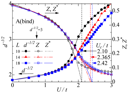
Figure 12: (Color online) The Mott critical value $U_{\rm c}/t$ for completely D-H bound state A(bind) is estimated in two ways. The vertical dashed lines indicate the values estimated from the extrapolation ($Z^{*}$) to zero of the quasiparticle renormalization factor $Z$. The other estimate is given by the crossing point of $\ell_{\rm DH}^{*}$ ($=3$) and $\ell_{\rm DD}^{*}$ ($=1/\sqrt{d}$). The results are listed in Table. 2.

For simplicity, we take up a one-dimensional case,[55] and first assume that $U/t$ is small and the doublon (and holon) density is sufficiently high. Actually, for $U/t\ \raise 1.50696pt\hbox{$<$}\kern-7.5pt\lower 2.15277pt\hbox{$\sim$}\ 1.5$, $d$ of $\Psi_{\rm A(bind)}$ becomes higher than those of the other D-H binding states [see Fig. 3(b)]. Then, a doublon are often accompanied by multiple holons in the NN sites, so that it can propagate independently of holons as a plus charge carrier, satisfying the complete binding condition:

$$[\cdot\cdot{\rm DH\dot{D}}_{\leftrightarrow}{\rm\dot{H}DH}\cdot\cdot]\rightarrow[\cdot\cdot{\rm DH}_{\leftrightarrow}{\rm\dot{H}\dot{D}}_{\leftrightarrow}{\rm DH}\cdot\cdot]\rightarrow\qquad$$

$$[\cdot\cdot{\rm D}_{\leftrightarrow}{\rm\dot{H}HD\dot{D}}_{\leftrightarrow}{\rm H}\cdot\cdot]\rightarrow[\cdot\cdot_{\leftrightarrow}{\rm\dot{H}DHDH\dot{D}}_{\leftrightarrow}\cdot\cdot]\rightarrow\qquad.$$ (24)

Here, pay attention to the dotted D and H, which propagate by exchanging the positions according to the double-headed arrows. Thus, the state becomes metallic. On the other hand, when $U/t$ becomes large and the doublon density becomes sufficiently low, most D-H pairs become mutually detached, as $[\cdot\cdot{\rm\uparrow\downarrow HD\downarrow\uparrow HD\uparrow\downarrow}\cdot\cdot].$ Then, a doublon becomes unable to propagate independently of holons, and vice versa, satisfying the completely bound condition. Consequently, charge fluctuation is confined locally, resulting in an insulator. Summing up, the conduction in a metallic state requires that D-H pairs should contact with one another in sequence; the Mott critical value can be specified by $U/t$ at which D-H pairs are mutually detached.

From the above argument, we find it convenient for general discussions of Mott transitions to introduce two characteristic length scales, the D-H binding length $\ell_{\rm DH}$ and the D-D exclusion length $\ell_{\rm DD}$, which are generally a function of $U/t$. We postulate that the attractive correlation factor $P_{\rm A}$ produces D-H pairs of a binding length $\ell_{\rm DH}$ according to $U/t$; $\ell_{\rm DH}$ approximately corresponds to the size of a D-H-pair domain, in which at least one doublon and one holon must exist. $\ell_{\rm DD}$ broadly represents the distance between two D-H pairs. Using $\ell_{\rm DH}$ and $\ell_{\rm DD}$, we give a microscopic picture of Mott transitions, which is schematically shown in Figs. 15(c) and (d) for general D-H binding wave functions. In the insulating phase, the relation $\ell_{\rm DH}<\ell_{\rm DD}$ holds, indicating that the domains of D-H pairs do not usually overlap, at least, not in sequence. Consequently, most D-H pairs are isolated and a doublon and a holon are confined within $\ell_{\rm DH}$, resulting in only local charge fluctuation. To this point, the picture is basically identical with the previous one.[37] In the conductive phase ($U<U_{\rm c}$), $\ell_{\rm DH}$ becomes larger than $\ell_{\rm DD}$, indicating the domains of D-H pairs overlap with one another. Then, a doublon in a D-H pair can exchange a partner holon with a holon in an adjacent D-H pair, when the two holons are in the overlapped area. As a result, a doublon and a holon can move independently as charge carriers by successively exchanging the partner. As $U/t$ is varied, a Mott transition takes place when $\ell_{\rm DH}$ becomes equivalent to $\ell_{\rm DD}$, which is roughly $1/\sqrt{d}$ and generally a monotonically increasing function of $U/t$. In this framework, it is of primarily important to determine $\ell_{\rm DH}$ and $\ell_{\rm DD}$ appropriately.

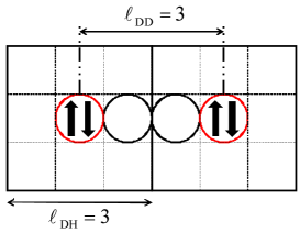
Figure 13: (Color online) Two domains of D-H pairs for the completely bound state A(bind) (domain size $\ell_{\rm DH}$ is 3) are schematically shown at the Mott critical case: $\ell_{\rm DD}=\ell_{\rm DH}$. Doublons and holons are represented by circles with and without arrows, respectively. The empty squares indicate singly occupied sites.

Now, we apply the above framework to the special case of $\Psi_{\rm A(bind)}$. We postulate that a domain of a D-H pair for $\Psi_{\rm A(bind)}$ consists of $3\times 3$ lattice sites, as shown in Fig. 13. Note that the size of this domain for $\Psi_{\rm A(bind)}$ is constant, irrespective of $U/t$, because a doublon and a holon (or holons) are tightly bound in the nearest neighbor site(s). For $\ell_{\rm DH}<3$, some domains of D-H pairs mutually overlap, and sequence like DHDHDH in (24) possibly appears, whereas for $\ell_{\rm DH}>3$ the domains of D-H pairs separate from each other on average. Thus, it seems appropriate to put $\ell_{\rm DH}^{*}=3$. Here, we add a star to distinguish it from the form for ordinary (not completely bound) $\Psi_{\rm A}$’s discussed later. As for the D-D exclusion length, we simply put $\ell_{\rm DD}^{*}=1/\sqrt{d}$, as mentioned above. In Fig. 12, we plot $\ell_{\rm DD}^{*}$ versus $U/t$. The values of $U/t$ at which $\ell_{\rm DH}^{*}=\ell_{\rm DD}^{*}$ are summarized in Table. 2, and approximately consistent with the Mott critical values estimated from $Z$. Thus, the above picture with a broad estimate of $\ell_{\rm DH}$ and $\ell_{\rm DD}$ yields a justifiable result to this special case.

4.2 Application to ordinary D-H wave functions

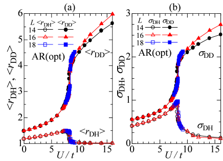
Figure 14: (Color online) (a) The nearest D-to-H and H-to-D distances and the nearest D-to-D and H-to-H distances calculated with AR(opt) are plotted for three system sizes as a function of the interaction strength. (b) Standard deviations of $\langle r_{\rm DH}\rangle$ and of $\langle r_{\rm DD}\rangle$ shown in (a).

Here, we study whether the above picture of Mott transitions is applicable to ordinary D-H binding (not rigidly bound) wave functions $\Psi_{\rm A}$ and to those with repulsive factors $\Psi_{\rm AR}$. In contrast to $\Psi_{\rm A(bind)}$, the distance from a doublon to its nearest holon(s), $\langle r_{\rm DH}\rangle$, varies in the ordinary $\Psi_{\rm A}$ and $\Psi_{\rm AR}$, so that not only $\ell_{\rm DD}$ but also $\ell_{\rm DH}$ should depend on $U/t$. In Fig. 14(a), we show the behavior of the averages of the nearest D-to-H and H-to-D distances $\langle r_{\rm DH}\rangle$ and of the nearest D-to-D and H-to-H distances $\langle r_{\rm DD}\rangle$ calculated with $\Psi_{\rm AR(opt)}$ are plotted as a function of $U/t$. Figure 14(b) shows the standard deviations of $\langle r_{\Lambda}\rangle$ ($\Lambda=$ DH or DD),

$$\sigma_{\Lambda}=\sqrt{\frac{1}{M}\sum_{i=1}^{M}(r_{i}-\langle r_{\Lambda}\rangle)^{2}},$$ (25)

where the index $i$ runs over all the doublons and holons in all the measured samples, and $M$ indicates their total number. $\sigma_{\Lambda}$ behaves similarly to $\langle r_{\Lambda}\rangle$. Allowing for the meaning of $\ell_{\rm DH}$ and $\ell_{\rm DH}$, we put, generally,

$$\ell_{\rm DH} = \langle r_{\rm DH}\rangle+\sigma_{\rm DH},$$ (26)

$$\ell_{\rm DD} = \langle r_{\rm DD}\rangle-\sigma_{\rm DD}.$$ (27)

Namely, $\ell_{\rm DH}$ broadly represents the maximum radius of a D-H pair domain, over which a doublon does not separate from holons, as in Fig. 15(a), and $\ell_{\rm DD}$ the minimum D-D length, under which doublons do not approach each other, as in Fig. 15(b).

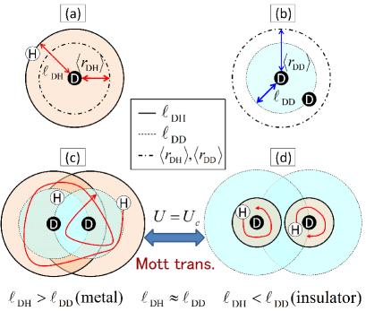
Figure 15: (Color online) Schematic figures of microscopic mechanism of the Mott transition. (a) The solid circle of radius $\ell_{\rm DH}$ denotes the domain in which a holon can itinerate, when the partner doublon is located at the center. (b) The solid circle of radius $\ell_{\rm DD}$ denotes the forbidden area where a doublon cannot enter, when another doublon is situated at the center. In (c) and (d), the behavior of doublons (D) and holons (H) is illustrated for metallic and insulating states, respectively, in ordinary D-H binding wave functions. The explanation is given in §4.1. The two phases are distinguished by comparing the magnitude of $\ell_{\rm DH}$ and $\ell_{\rm DD}$.

In the metallic regime, $\langle r_{\rm DH}\rangle$ and $\sigma_{\rm DH}$ gradually increase as $U/t$ increases as shown in Fig. 14, chiefly because the densities of doublon and holon are reduced by $U/t$ [see Fig. 3(b)]. This effect exceeds the D-H binding effect of $P_{\rm A}$. Consequently, a doublon somewhat separate from holons. At the Mott critical point, however, $\langle r_{\rm DH}\rangle$ and $\sigma_{\rm DH}$ suddenly drop, and asymptotically approach 1 and 0, respectively, in the insulating regime, owing to the predominant D-H binding effect. In contrast, $\langle r_{\rm DD}\rangle$ and $\sigma_{\rm DD}$ monotonically increase as $U/t$ increases, owing to the steady decrease of $d$. In Fig. 16, $\ell_{\rm DH}$ and $\ell_{\rm DD}$ obtained through eqs. (26) and (27) are plotted. The Mott critical points $U_{\rm c}/t$ are estimated from the steepest descent of an order parameter of the Mott transition $d$, and are listed in Table 2. It is found that $\ell_{\rm DH}$ intersects $\ell_{\rm DH}$ almost at $U_{\rm c}/t$. Namely, the Mott critical point is estimated also from the condition,

$$\ell_{\rm DH}=\ell_{\rm DD}.$$ (28)

The values of $U_{\rm c}/t$ thus obtained are listed in Table 2. Thus, the picture of the Mott transition introduced in §4.1 [Figs. 15(c) and 15(d)] is applicable to $\Psi_{\rm AR(opt)}$.

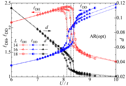
Figure 16: (Color online) The D-H binding length $\ell_{\rm DH}$ and the D-D exclusion distance $\ell_{\rm DD}$ for AR(opt) obtained from the data in Fig. 14 are plotted as a function of $U/t$. For comparison, the doublon density and the critical values obtained thereby (vertical dashed lines) are added for the same systems.

Now, we confirm whether the above scheme with eqs. (26) and (27) are effective also for other wave functions. We have made similar analyses for various types of $\Psi_{\rm A}$ and $\Psi_{\rm AR}$ in Table 1. As a results, the Mott critical values determined under the condition eq. (28) coincides with $U/t$ estimated from $d$ for every wave function with sufficient accuracy at least for large $L$. As an example, in Fig. 17, we plot the same quantities as in Fig. 16 for four representatives.

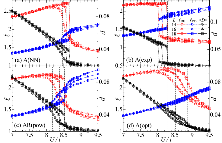
Figure 17: (Color online) The same quantities as in Fig. 16 ($\ell_{\rm DH}$, $\ell_{\rm DD}$, $d$) are shown in the same way for four different types of wave functions: (a) A(NN), (b) A(exp), (c) AR(pow) and (d) A(opt). The symbols indicated in (b) are common to all panels. The Mott critical values $U_{c}/t$ obtained by $d$ and the crossing point of $\ell_{\rm DH}$ and $\ell_{\rm DD}$ are summarized in Table. 2.

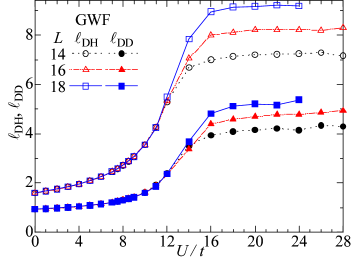
Figure 18: (Color online) D-H binding length $\ell_{\rm DH}$ and D-D exclusion distance $\ell_{\rm DD}$ calculated with Gutzwiller wave function as function of interaction strength.

Finally, we touch on the wave functions with only repulsive correlation factors, namely GWF and the three $\Psi_{\rm R}$’s in Table 1. As mentioned in §3.5, these wave functions do not undergo Mott transitions, and are always metallic for $U/t<\infty$. In Fig. 18, we plot $\ell_{\rm DH}$ and $\ell_{\rm DD}$ of GWF versus $U/t$, as a typical example. $\ell_{\rm DD}$ is a monotonically increasing function of $U/t$ in the similar way as $\Psi_{\rm A}$ and $\Psi_{\rm AR}$, whereas $\ell_{\rm DH}$ is also a monotonically increasing function and is always about twice larger than $\ell_{\rm DD}$. Namely, the relation $\ell_{\rm DH}>\ell_{\rm DD}$ always holds and $\ell_{\rm DH}$ never crosses $\ell_{\rm DD}$. The situation is the same for the three $\Psi_{\rm R}$’s. Thus, the new picture on the Mott transition properly works for the repulsive Jastrow-type wave functions. From this argument, it is certified again that the D-H binding effect is the essence of the Mott transition.

5 Summary

In this paper, we have studied the nonmagnetic Mott transition in the Hubbard model on the square lattice, using a variational Monte Carlo method. In the trial wave functions, we introduce long-range doublon-holon attractive and doublon-doublon (holon-holon) repulsive correlation factors, in addition to the onsite repulsive factor. We recapitulate the main results below.

(1) We confirmed that the D-H binding correlation is crucial to describe first-order nonmagnetic Mott transitions. The D-H attractive projector, if properly chosen, considerably reduces the variational energy for $U\ \raise 1.50696pt\hbox{$>$}\kern-7.5pt\lower 2.15277pt\hbox{$\sim$}\ W$.

(2) We clarified the optimized weight of the D-H binding factor $f_{\rm A}(r)$, which rapidly decreases for $r\ \raise 1.50696pt\hbox{$<$}\kern-7.5pt\lower 2.15277pt\hbox{$\sim$}\ 3$, but becomes almost constant for $r\ \raise 1.50696pt\hbox{$>$}\kern-7.5pt\lower 2.15277pt\hbox{$\sim$}\ 3$ in the metallic regime. Thereby, it becomes clear why the simple conventional short-range D-H factors capture the essence of the Mott transition. In the insulating regime, the D-H binding factor becomes very short-ranged; consequently, charge fluctuation, i.e. D-H pairs, is confined within $r\ \raise 1.50696pt\hbox{$<$}\kern-7.5pt\lower 2.15277pt\hbox{$\sim$}\ 2$.

(3) The D-D repulsive factors improve the energy only slightly, especially in the metallic regime, and do not induce a Mott transition by itself. However, the improvement in the insulating regime contributes to some downward shift of the Mott critical point $U_{\rm c}/t$.

(4) Motivated by the Mott transition in the completely D-H bound state, we have renewed the picture of Mott transitions. Two characteristic length scales $\ell_{\rm DH}$ and $\ell_{\rm DD}$ are introduced; $\ell_{\rm DH}$ broadly represents the size of a D-H pair, and $\ell_{\rm DD}$ the minimum distance between two doublons. The two lengths generally depend largely on $U/t$, and should be appropriately estimated. The Mott critical point determined by the condition $\ell_{\rm DH}=\ell_{\rm DD}$ is consistent with the values estimated from other quantities. This picture is applicable to a wide range of Mott transitions including the Bose Hubbard model.[39]

We leave some intriguing subjects for future studies: (i) Improvement of the critical point $U_{\rm c}/t$. (ii) Introduction of explicit AF and superconducting correlation into the one-body part.[56] (iii) How the new picture works for doped cases, namely, doped Mott insulators like the cuprate superconductors.

- [1] N. F. Mott: Metal-insulator transitions, (Taylor & Francis, London, 1990).
- [2] M. Greiner, O. Mandel, T. Esslinger, T. W. Hänsch and I. Bloch: Nature 415 (2002) 39.
- [3] T. Stöferle, H. Moritz, C. Schori, M. Köhl and T. Esslinger: Phys. Rev. Lett. 92 (2004) 130403.
- [4] M. Köhl, H. Moritz, T. Stöferle, C. Schori and T. Esslinger: J. Low Temp. Phys. 138 (2005) 635.
- [5] I. B. Spielman, W. D. Phillips and J. V. Porto: Phys. Rev. Lett. 98 (2007) 080404.
- [6] For instance, M. P. A. Fisher, P. B. Weichman, G. Grinstein and D. S. Fisher: Phys. Rev. B 40 (1989) 546.
- [7] D. Jaksch, C. Bruder, J. I. Cirac, C. W. Gardiner and P. Zoller: Phys. Rev. B 81 (1998) 3108.
- [8] I. Bloch, J. Dalibard and W. Zwerger: Rev. Mod. Phys. 80 (2008) 885.
- [9] At unit filling, the critical value is estimated at in one dimension (ref. \citenUc-1d), at 16.4-16.7 for the square lattice (ref.\citenQMC-2D1,QMC-2D2,QMC-2D3,Monien), and at 29.3 (ref. \citenUc-3d1) or 31.3 (ref. \citenUc-3d2) for the simple cubic lattice.
- [10] T. D. Kühner and H. Monien: Phys. Rev. B 58 (1998) R14741.
- [11] W. Krauth and N. Trivedi: Europhys. Lett. 14 (1991) 627.
- [12] S. Wessel, F. Alet, M. Troyer and G. G. Batrouni: Phys. Rev. A 70 (2004) 053615.
- [13] B. Capogrosso-Sansone, S. G. Söyler, N. Prokof’ev and B. Svistunov: Phys. Rev. A 77 (2008) 015602.
- [14] N. Elstner and H. Monien: Phys. Rev. B 59 (1999) 12184.
- [15] B. Capogrosso-Sansone, N. V. Prokof’ev and B. V. Svistunov: Phys. Rev. B 75 (2007) 134302.
- [16] Y. Kato, Q. Zhou, N. Kawashima and N. Trivedi: Nat. Phys. 4 (2008) 617.
- [17] J. C. Slater: Phys. Rev. 82 (1951) 538.
- [18] K. Kanoda: Physica C 282-287 (1997) 299; K. Miyagawa, K. Kanoda and A. Kawamoto: Chem. Rev. 104 (2004) 5635; R. H. McKenzie: Science 278 (1997) 820.
- [19] P. A. Lee, N. Nagaosa and X. -G. Wen: Rev. Mod. Phys. 78 (2006) 17.
- [20] M. Ogata and H. Fukuyama: Rep. Prog. Phys. 71 (2008) 036501.
- [21] H. Yokoyama, M. Ogata, Y. Tanaka, K. Kobayashi and H. Tsuchiura: in preparation.
- [22] J. E. Hirsch and D. J. Scalapino: Phys. Rev. B 27 (1983) 7169.
- [23] H. Yokoyama and H. Shiba: J. Phys. Soc. Jpn. 56 (1987) 3582
- [24] M. Gutzwiller: Phys. Rev. Lett. 10 (1963) 159.
- [25] W. F. Brinkman and T. M. Rice: Phys. Rev. B 2 (1970) 4302.
- [26] W. L. McMillan: Phys. Rev. 138 (1965) A442.
- [27] D. Ceperley, G. V. Chester, K. H. Kalos, Phys. Rev. B 16 (1977) 3081.
- [28] H. Yokoyama and H. Shiba: J. Phys. Soc. Jpn. 56 (1987) 1490.
- [29] M. Gutzwiller, Phys. Rev. 137 (1965) A1726.
- [30] W. Metzner and D. Vollhardt; Phys. Rev. B 37 (1988) 7382.
- [31] T. A. Kaplan, P. Horsch and P. Fulde: Phys. Rev. Lett. 49 (1982) 889.
- [32] P. Fazekas and K. Penc: Int. J. Mod. Phys. B1 (1988) 1021; P. Fazekas, Physica Scripta T 29 (1989) 125.
- [33] H. Yokoyama and H. Shiba: J. Phys. Soc. Jpn. 59 (1990) 3669.
- [34] H. Yokoyama: Prog. Theor. Phys. 108 (2002) 59.
- [35] H. Yokoyama, Y. Tanaka, M. Ogata and H. Tsuchiura: J. Phys. Soc. Jpn. 73 (2004) 1119.
- [36] T. Watanabe, H. Yokoyama, Y. Tanaka and J. Inoue: J. Phys. Soc. Jpn. 75 (2006) 074707.
- [37] H. Yokoyama, M. Ogata and Y. Tanaka: J. Phys. Soc. Jpn. 75 (2006) 114706.
- [38] M. Capello, F. Becca, S. Yunoki and S. Sorella: Phys. Rev. B 73 (2006) 245116.
- [39] H. Yokoyama, T. Miyagawa and M. Ogata: to appear in Physica C (2011), and submitted to J. Phys. Soc. Jpn..
- [40] T. Miyagawa and H. Yokoyama: to appear in Physica C (2011).
- [41] J. Hubbard: Proc. Roy. Soc. A267 (1963) 237.
- [42] J. Kanamori: Prog. Theor. Phys. 30 (1963) 275.
- [43] See also, A. Georges, G. Kotliar, W. Krauth and M. J. Rozenberg: Rev. Mod. Phys. 68 (1996) 13.
- [44] C. Castellani, C. Di Castro, D. Feinberg and J. Ranninger: Phys. Rev. Lett. 43 (1979) 1957.
- [45] E. H. Lieb and F. Y. Wu: Phys. Rev. Lett. 20 (1968) 1445.
- [46] For instance, A. B. Harris and R. V. Range: Phys. Rev. 157 (1967) 295.
- [47] M. Capello, F. Becca, M. Fabrizio, S. Sorella and E. Tosatti: Phys. Rev. Lett. 94 (2005) 026406.
- [48] C. J. Umrigar, K. G. Wilson and J. W. Wilkins: Phys. Rev. Lett. 60 (1988) 1719.
- [49] C. J. Umrigar and C. Filippi: Phys. Rev. Lett. 94 (2005) 150201; S. Sorella: Phys. Rev. B 71 (2005) 241103.
- [50] For instance, R. Fletcher: Practical Methods of Optimization 2nd ed., (John Wily, 1987).
- [51] T. Ibaraki and M. Fukushima: FORTRAN77 Optimization Programming, chap. 6 (Iwanami, Tokyo, 1991), [in Japanese].
- [52] C. S. Hellberg and E. J. Mele: Phys. Rev. Lett. 67 (1991) 2080.
- [53] As known from in Fig. 11(b), the repulsive correlation factor for the NN sites is useless. The reasons why in Fig. 8(b) is the smallest for are probably (i) a holon(s) occupies the NN sites of the doublon [Fig. 11(a)], and (ii) the effect of exchange hole is conspicuous for .
- [54] for (not shown) behaves basically like , but, for , slowly decreases to unity as increases.
- [55] In fact, we have confirmed that A(bind) is insulating for any positive value of in the one-dimensional Hubbard model.
- [56] For instance, D. Tahara and M. Imada: J. Phys. Soc. Jpn. 77 (2008) 093703, and J. Phys. Soc. Jpn. 77 (2008) 114701.