Frontier estimation with local polynomials and high power-transformed data

Abstract

We present a new method for estimating the frontier of a sample. The estimator is based on a local polynomial regression on the power-transformed data. We assume that the exponent of the transformation goes to infinity while the bandwidth goes to zero. We give conditions on these two parameters to obtain almost complete convergence. The asymptotic conditional bias and variance of the estimator are provided and its good performance is illustrated on some finite sample situations.

Keywords: local polynomials estimator, power-transform, frontier estimation.

AMS 2000 subject classification: 62G05, 62G07, 62G20.

1 Introduction

Let $\left(X_{i},Y_{i}\right)$, $i=1,...,n$ be independent and identically distributed continuous variables and suppose that their common density has a support defined by

$$S=\left\{\left(x,y\right)\in\mathbb{R}\times\mathbb{R};0\leq y\leq g\left(x\right)\right\}.$$

The unknown function $g$ is called the frontier. We address the problem of estimating $g$. In [13], we introduced a new kind of estimator based upon kernel regression on high power-transformed data. More precisely the estimator of $g(x)$ was defined by

$$\left(\left(p+1\right)\sum_{i=1}^{n}K_{h}\left(X_{i}-x\right)Y_{i}^{p}\left/\sum_{i=1}^{n}K_{h}\left(X_{i}-x\right)\right.\right)^{1/p}$$

where $p=p_{n}\rightarrow\infty$ and $h=h_{n}\rightarrow 0$ are non random sequences, $K$ is a symmetrical probability density with support included in $\left[-1,1\right]$, and $K_{h}(\bullet)=K\left(\bullet/h\right)/h$. Although the correcting term $\left(p+1\right)^{1/p}$ was specially designed to deal with the case of a uniform conditional distribution of $Y/X=x$, this estimate has been shown to converge in any case. In the special but interesting case of a uniform conditional distribution of $Y/X=x$ for a $\alpha-$lipschitzian frontier the minimax rate of convergence is attained. We also proved that the estimator is asymptotically Gaussian. It is also interesting to note that, compared to the extreme value based estimators [7, 8, 10, 11, 14, 12], projection estimators [18] or piecewise polynomial estimators [21, 20, 17], this estimator does not require a partition of the support $S$.

A natural idea suggested by our referees was to investigate the possible gains obtained by substituting a local polynomial regression to the Nadaraya-Watson regression. The basic idea in this theory consists in approximating locally a $C_{k+1}$ regression function by a polynomial of degree $k$ and taking the zero-degree term as an estimate of the regression. The regularity of the function brings improvement on the bias term. Accordingly, when dealing with high power-transformed data we establish in this paper that the bias of the local polynomial estimator of degree $k$ is $O_{p}(h(hp)^{k})$ and the variance is $O_{p}\left(1/nhp\right)$.

Let us introduce the notations $Z=\left(p+1\right)Y^{p}$ and $r_{n}\left(x\right)=\mathbb{E}\left(Z/X=x\right)$. The conditional distribution of $Y/X=x$ is supposed to be uniform on $\left[0,g\left(x\right)\right]$, so that $r_{n}\left(x\right)=g^{p}\left(x\right)$. For fixed $p$ the method for estimating $r_{n}\left(x\right)$ first consists in solving the following minimization problem

$$\underset{\beta_{0},...,\beta_{k}}{\arg\min}\sum_{i=1}^{n}\left(\left(p+1\right)Y_{i}^{p}-\sum_{j=0}^{k}\beta_{j}\left(X_{i}-x\right)^{j}\right)^{2}K_{h}\left(X_{i}-x\right)\text{.}$$ (1)

Then, denoting by $\widehat{\mathbf{\beta}}=(\widehat{\beta}_{0},...,\widehat{\beta}_{k})^{t}$ the solution of this least square minimization, one considers $\widehat{\beta}_{0}$ as an estimate of $r_{n}\left(x\right)=\mathbb{E}\left(Z/X=x\right)$. The originality and the difficulty of our paper in contrast with these traditional lines is that here $p=p_{n}\rightarrow\infty$ and that we consider $\widehat{\beta}_{0}^{1/p}$ as an estimate of $g\left(x\right).$ So we write $\widehat{g}_{n}\left(x\right)=\widehat{\beta}_{0}^{1/p}=\widehat{r}_{n}^{1/p}\left(x\right)$. We refer to [16, 15, 19] for other definitions of local polynomials estimators (i.e. without high power transform) and to [3, 6, 9, 1, 2] for the estimation of frontier functions under monotonicity assumptions.

In order to get simplified matricial expressions, let us denote by $\mathbf{X}$ the $n\times\left(k+1\right)$ matrix defined by the lines $[1,X_{i}-x,...,\left(X_{i}-x\right)^{k}]_{i=1,...n}$. The diagonal matrix of weights $diag\left\{K_{h}\left(X_{i}-x\right)\right\}$ is denoted by $\mathbf{W}$. We call design the vector$\ \mathcal{X}=(X_{1},...,X_{n})^{t}$ and we denote by $\mathcal{Z}$ the vector $\left(Z_{1},...,Z_{n}\right)^{t}$. Then the local regression problem $\left(\ref{1-0}\right)$ can be rewritten as

$$\widehat{\mathbf{\beta}}=\arg\min_{\beta}\left(\mathcal{Z}\mathbf{-X\beta}\right)^{t}\mathbf{W}\left(\mathcal{Z}\mathbf{-X\beta}\right),$$

where $\beta=(\beta_{0},\dots,\beta_{k})^{t}$. It is well known from the weighted least square theory that

$$\widehat{\mathbf{\beta}}=\left(\mathbf{X}^{t}\mathbf{WX}\right)^{-1}\mathbf{X}^{t}\mathbf{W}\mathcal{Z}.$$

In particular, in the case $k=0$ we have

$$\widehat{\mathbf{\beta}}=\widehat{\beta}_{0}=\sum_{i=1}^{n}Z_{i}K_{h}\left(X_{i}-x\right)\left/\sum_{i=1}^{n}K_{h}\left(X_{i}-x\right)\right.,$$

so we exactly find back the estimator $\widehat{g}_{n}\left(x\right)=\widehat{\beta}_{0}^{1/p}$ studied in [13]. In order to give a general expression of $\widehat{r}_{n}\left(x\right)$, we adopt the notations of Fan and Gijbels whose book [5] will also serve of reference for some preliminary results established in Section 2 (see also [22] for a general multidimensional analysis). Basing on this, the asymptotic conditional bias and variance of the estimator are derived in Section 3 when $Y$ given $X=x$ is uniformly distributed. This result is extended in Section 4, where the almost complete convergence is proved without this uniformity assumption. We conclude this paper by an illustration of the behavior of our estimator on some finite sample situations in Section 5. Technical lemmas are postponed to the appendix.

2 Preliminary results

Let $x\in{\mathbb{R}}$. From now on, it is assumed that the density function $f$ of $X_{1}$ is continuous at $x$ and that $f(x)>0$. Besides, we suppose that there exists $g_{\min}>0$ such that, for all $t\in{\mathbb{R}}$, $g_{\min}\leq g(t)$. Let $\mathbf{S}_{n}=\mathbf{X}^{t}\mathbf{WX}$ be the $\left(k+1\right)\times\left(k+1\right)$ matrix $\left[S_{n,j+l}\right]$ _0≤j,l≤k defined by

$$S_{n,j}=\sum_{i=1}^{n}\left(X_{i}-x\right)^{j}K_{h}\left(X_{i}-x\right).$$

Similarly, denoting by $\mathbf{\Sigma}$ the $n\times n$ diagonal matrix $diag\left\{K_{h}^{2}\left(X_{i}-x\right)g^{2p}\left(X_{i}\right)\right\}$, $\mathbf{S}_{n}^{\ast}~{}=\mathbf{X}^{t}\mathbf{\Sigma X}$ is the $\left(k+1\right)\times\left(k+1\right)$ matrix $[S_{n,j+l}^{\ast}]_{0\leq j,l\leq k}$ with

$$S_{n,j}^{\ast}=\sum_{i=1}^{n}\left(X_{i}-x\right)^{j}K_{h}^{2}\left(X_{i}-x\right)g^{2p}\left(X_{i}\right).$$

Finally, we introduce the matrices $\mathbf{S}=\left[\mu_{j+l}\right]_{0\leq j,l\leq k}$ and $\mathbf{S}^{\ast}=$ $\left[\nu_{j+l}\right]_{0\leq j,l\leq k}$ with $\mu_{j}=\int u^{j}K\left(u\right)du$ and $\nu_{j}=\int u^{j}K^{2}\left(u\right)du$. Following roughly the same lines as Fan and Gijbels [5], we obtain asymptotic expressions for $S_{n,j}$ and $S_{n,j}^{\ast}$. The first equality (2) is a standard result of the theory and the second one (3) boils down to an easy adaptation. Proofs are thus omitted.

Proposition 1

If $h\rightarrow 0$ and $nh\rightarrow\infty$, then

$$S_{n,j}=nh^{j}f\left(x\right)\mu_{j}\left[1+o_{p}\left(1\right)\right].$$ (2)

If, moreover, $ph\rightarrow 0$ we have for any $C_{1}$ function $g$

$$S_{n,j}^{\ast}=nh^{j-1}g^{2p}\left(x\right)f\left(x\right)\nu_{j}\left[1+o_{p}\left(1\right)\right]\text{.}$$ (3)

Let us now quote a general expression of the conditional bias of$\ \widehat{r}_{n}\left(x\right)$. From Fan and Gijbels [5], and denoting by $e_{1}=(1,0,...,0)^{t}$ the first vector of the canonical basis of $\mathbb{R}^{k+1}$, we have

$$r_{n}\left(x\right) = \beta_{0}=e_{1}^{t}\beta\mathbf{~{}=}~{}e_{1}^{t}\mathbf{S}_{n}^{-1}\mathbf{X}^{t}\mathbf{WX\beta,}$$

$$\widehat{r}_{n}\left(x\right) = \widehat{\beta}_{0}=e_{1}^{t}\widehat{\mathbf{\beta}}=e_{1}^{t}\mathbf{S}_{n}^{-1}\mathbf{X}^{t}\mathbf{W}\mathcal{Z},$$

so that

$$\mathbb{E}\left(\widehat{r}_{n}\left(x\right)/\mathcal{X}\right)-r_{n}\left(x\right)=e_{1}^{t}\mathbf{S}_{n}^{-1}\mathbf{X}^{t}\mathbf{W}\left[\mathbb{E}\left(\mathcal{Z}/\mathcal{X}\right)-\mathbf{X\beta}\right].$$ (4)

In Appendix I we give a detailed proof of the following

Proposition 2

Suppose $g$ is a $C_{k+1}$ function. If $h\rightarrow 0$, $nh\rightarrow\infty$ and $ph\rightarrow 0$, then

$$\mathbb{E}\left(\frac{\widehat{r}_{n}\left(x\right)}{r_{n}\left(x\right)}-1/\mathcal{X}\right)=O_{p}\left(\left(hp\right)^{k+1}\right).$$

We now examine the conditional variance of $\widehat{r}_{n}\left(x\right)$

$$\mathbb{V}\left(\widehat{r}_{n}\left(x\right)/\mathcal{X}\right)=e_{1}^{t}\mathbf{S}_{n}^{-1}\mathbf{X}^{t}\mathbb{V}\mathbf{\left(\mathbf{W}\mathcal{Z}\mathbf{/}\mathcal{X}\right)XS}_{n}^{-1}e_{1}.$$

Taking into account of the independence of the pairs $\left(X_{i},Y_{i}\right),\mathbb{V}\mathbf{\left(\mathbf{W}\mathcal{Z}\mathbf{/}\mathcal{X}\right)}$ is the diagonal matrix $diag\left\{K_{h}^{2}\left(X_{i}-x\right)\mathbb{V}(Z_{i}/X_{i}=x)\right\}$. From the uniformity of the conditional distribution of the $Y_{i}/X_{i}=x$, it is easily seen that $\mathbb{V}(Z_{i}/X_{i}=x)=\frac{p^{2}}{2p+1}g^{2p}\left(x\right)$, so that

$$\mathbb{V}\left(\widehat{r}_{n}\left(x\right)/\mathcal{X}\right)=\frac{p^{2}}{2p+1}e_{1}^{t}\mathbf{S}_{n}^{-1}\mathbf{S}_{n}^{\ast}\mathbf{S}_{n}^{-1}e_{1}.$$

Following the same lines as Fan and Gijbels [5], we obtain the following asymptotic expression

Proposition 3

Suppose $g$ is a $C_{k+1}$ function. If $h\rightarrow 0$, $nh\rightarrow\infty$ and $ph\rightarrow 0$, then

$$\mathbb{V}\left(\frac{\widehat{r}_{n}\left(x\right)}{r_{n}\left(x\right)}/\mathcal{X}\right)=\frac{C}{f\left(x\right)}\frac{1}{nh}\frac{p^{2}}{2p+1}\left[1+o_{p}\left(1\right)\right],$$

where $C=e_{1}^{t}\mathbf{S}^{{}^{-1}}\mathbf{S}^{\ast}\mathbf{S}^{{}^{-1}}e_{1}$.

The proof of Proposition 3 is much easier than the one of Proposition 2 and it thus omitted.

3 Conditional bias and variance of $\widehat{g}_{n}\left(x\right)$

Here we present the main results of this paper and an outline of their proofs. Many details and ancillary results are postponed to Appendix II. Proofs are made under the assumption that $g$ is a $C_{k+1}$ function and the system of conditions below

$$H:\begin{bmatrix}n\rightarrow\infty,~{}h\rightarrow 0,~{}p\rightarrow\infty\\ nh\rightarrow\infty,~{}hp\rightarrow 0\\ \left(p/nh\right)\log^{2}(nh)\sim\left(hp\right)^{2k+2}\end{bmatrix}.$$

Theorem 1

Suppose $H$ holds and $g$ is a $C_{k+1}$ function. Then, the asymptotic conditional bias of the estimate is given by

$$\mathbb{E}\left(\frac{\widehat{g}_{n}\left(x\right)}{g\left(x\right)}-1/\mathcal{X}\right)=O_{p}\left(h\left(hp\right)^{k}\right).$$

Proof. Let us write $w_{n}\left(x\right)=\widehat{r}_{n}\left(x\right)/r_{n}\left(x\right)-1$, so that $\widehat{g}_{n}\left(x\right)/g\left(x\right)=\left(1+w_{n}\left(x\right)\right)^{1/p}$ and define

$$\Delta_{n}=\left|\left(1+w_{n}\left(x\right)\right)^{1/p}-\left(1+\frac{w_{n}\left(x\right)}{p}\right)\right|.$$ (5)

Let $\alpha_{n}=\left(p/nh\right)^{1/4}$. For sufficiently large $n$ we have $\alpha_{n}<1/2$, and thus, Lemma 9 entails

$$\Delta_{n}\mathbf{1}\left\{\left|w_{n}\left(x\right)\right|<\alpha_{n}\right\}<c_{6}\frac{1}{p}w_{n}^{2}\left(x\right),$$ (6)

which leads to the following bound

$$\mathbb{E}\left(\Delta_{n}\mathbf{1}\left\{\left|w_{n}\left(x\right)\right|<\alpha_{n}\right\}/\mathcal{X}\right)\leq c_{6}\frac{\alpha_{n}}{p}\mathbb{E}\left(\left|w_{n}\left(x\right)\right|/\mathcal{X}\right)\leq c_{6}\frac{\alpha_{n}}{p}\mathbb{E}^{1/2}\left(w_{n}^{2}\left(x\right)/\mathcal{X}\right).$$

Now, from Proposition 2 and Proposition 3,

$$\mathbb{E}\left(w_{n}^{2}\left(x\right)/\mathcal{X}\right) =\mathbb{V}\left(\frac{\widehat{r}_{n}\left(x\right)}{r_{n}\left(x\right)}/\mathcal{X}\right)+\mathbb{E}^{2}\left(\frac{\widehat{r}_{n}\left(x\right)}{r_{n}\left(x\right)}-1/\mathcal{X}\right)$$

$$=\frac{c_{6}}{f\left(x\right)}\frac{1}{nh}\frac{p^{2}}{2p+1}\left[1+o_{p}\left(1\right)\right]+O_{p}\left(\left(hp\right)^{2k+2}\right)\text{.}$$

Then, taking into account of $h\left(hp\right)^{k}\sqrt{nhp}=\sqrt{\log(nh)}\rightarrow\infty$, it follows that

$$\mathbb{E}\left(\Delta_{n}\mathbf{1}\left\{\left|w_{n}\left(x\right)\right|<\alpha_{n}\right\}/\mathcal{X}\right) \leq c_{6}\frac{\alpha_{n}}{p}\left[O_{p}\left(\frac{p}{nh}\right)+O_{p}\left(\left(hp\right)^{2k+2}\right)\right]^{1/2}$$

$$=O_{p}\left(\alpha_{n}/\sqrt{nhp}\right)+O_{p}\left(\alpha_{n}h\left(hp\right)^{k}\right)$$

$$=O_{p}\left(\alpha_{n}h\left(hp\right)^{k}\right).$$ (7)

Besides, making use of Lemma 7, we can write

$$\mathbb{E}\left(\Delta_{n}\mathbf{1}\left\{\left|w_{n}\left(x\right)\right|\geq\alpha_{n}\right\}/\mathcal{X}\right)\leq c_{5}\left(\mathcal{X}\right)\mathbb{P}\left\{\left|w_{n}\left(x\right)\right|\geq\alpha_{n}/\mathcal{X}\right\},$$

and, from the triangular inequality,

$$\mathbb{P}\left\{\left|w_{n}\left(x\right)\right|\geq\alpha_{n}/\mathcal{X}\right\} \leq\mathbb{P}\left\{2\left|w_{n}\left(x\right)-\mathbb{E}\left(w_{n}\left(x\right)/\mathcal{X}\right)\right|\geq\alpha_{n}/\mathcal{X}\right\}$$

$$+\mathbb{P}\left\{2\left|\mathbb{E}\left(w_{n}\left(x\right)/\mathcal{X}\right)\right|\geq\alpha_{n}/\mathcal{X}\right\}.$$

Recalling that

$$\mathbb{E}\left(w_{n}\left(x\right)/\mathcal{X}\right)=\mathbb{E}\left(\frac{\widehat{r}_{n}\left(\mathcal{X}\right)}{r_{n}\left(\mathcal{X}\right)}-1/\mathcal{X}\right)=O_{p}\left(\left(hp\right)^{k+1}\right),$$

and noticing that $\left(hp\right)^{k+1}/\alpha_{n}=\left(p/nh\right)^{1/4}\left(\log(nh)\right)^{1/2}\rightarrow 0$, we conclude that the sequence $\mathbb{P}\left\{2\left|\mathbb{E}\left(w_{n}\left(x\right)/\mathcal{X}\right)\right|\geq\alpha_{n}/\mathcal{X}\right\}$ goes to $0$. Moreover, remark that $\mathbb{P}\left\{2\left|\mathbb{E}\left(w_{n}\left(x\right)/\mathcal{X}\right)\right|\geq\alpha_{n}/\mathcal{X}\right\}$ is a $\left\{0,1\right\}$-valued random variable. This means that for a sufficient large $n$ depending on $\mathcal{X}$, we merely have

$$\mathbb{P}\left\{2\left|\mathbb{E}\left(w_{n}\left(x\right)/\mathcal{X}\right)\right|\geq\alpha_{n}/\mathcal{X}\right\}=0.$$

Now, from Lemma 6,

$$\mathbb{P}\left(2\left|w_{n}\left(x\right)-\mathbb{E}\left(w_{n}\left(x\right)/\mathcal{X}\right)\right|\geq\alpha_{n}/\mathcal{X}\right)$$

$$=\mathbb{P}\left(\left|\widehat{r}_{n}\left(x\right)-\mathbb{E}\left(\widehat{r}_{n}\left(x\right)/\mathcal{X}\right)\right|\geq\frac{1}{2}\alpha_{n}r_{n}\left(x\right)/\mathcal{X}\right)$$

$$\leq 2\exp\left\{-c_{4}\frac{nh}{p}\frac{\alpha_{n}^{2}}{4}\left[1+o_{p}\left(1\right)\right]\right\}$$

$$=2\exp\left\{-\frac{c_{4}}{4}\sqrt{nh/p\log^{2}(nh)}\left[1+o_{p}\left(1\right)\right]\log(nh)\right\}$$

$$=\left(nh\right)^{-\infty_{p}\left(1\right)},$$

where $\infty_{p}\left(1\right)$ stands for a sequence going almost surely to the infinity. We thus have at least

$$\mathbb{E}\left(\Delta_{n}\mathbf{1}\left\{\left|w_{n}\left(x\right)\right|\geq\alpha_{n}\right\}/\mathcal{X}\right)=O_{p}\left(1/nh\right).$$ (8)

Collecting $\left(\ref{2-1}\right)$ and $\left(\ref{2-2}\right)$ yields

$$\mathbb{E}\left(\Delta_{n}/\mathcal{X}\right)=O_{p}\left(\alpha_{n}h\left(hp\right)^{k}\right)+O_{p}\left(1/nh\right).$$

From

$$\left|\mathbb{E}\left(\frac{\widehat{g}_{n}\left(x\right)}{g\left(x\right)}-1/\mathcal{X}\right)-\frac{1}{p}\mathbb{E}\left(w_{n}\left(x\right)/\mathcal{X}\right)\right|\leq\mathbb{E}\left(\Delta_{n}/\mathcal{X}\right)$$

and Proposition 2, we obtain

$$\mathbb{E}\left(\frac{\widehat{g}_{n}\left(x\right)}{g\left(x\right)}-1/\mathcal{X}\right) =\frac{1}{p}\mathbb{E}\left(w_{n}\left(x\right)/\mathcal{X}\right)+O_{p}\left(\alpha_{n}h\left(hp\right)^{k}\right)+O_{p}\left(1/nh\right)$$

$$=O_{p}\left(h\left(hp\right)^{k}\right)+O_{p}\left(1/nh\right).$$ (9)

Finally, since $h\left(hp\right)^{k}nh=\left(nh/p\right)\left(hp\right)^{k+1}=\sqrt{nh/p}\log(nh)\rightarrow\infty$, expansion $\left(\ref{2-3}\right)$ reduces to

$$\mathbb{E}\left(\frac{\widehat{g}_{n}\left(x\right)}{g\left(x\right)}-1/\mathcal{X}\right)=O_{p}\left(h\left(hp\right)^{k}\right),$$

and the conclusion follows.   

Theorem 2

Suppose $H$ holds and $g$ is a $C_{k+1}$ function. Then, the asymptotic conditional variance of the estimate is given by

$$\mathbb{V}\left(\frac{\widehat{g}_{n}\left(x\right)}{g\left(x\right)}-1/\mathcal{X}\right)=O_{p}\left(\frac{1}{nhp}\right).$$

Proof. Introducing

$$\delta=\frac{\widehat{g}_{n}\left(x\right)}{g\left(x\right)}-1-\frac{w_{n}\left(x\right)}{p},$$

we have

$$\mathbb{V}\left(\frac{\widehat{g}_{n}\left(x\right)}{g\left(x\right)}/\mathcal{X}\right)\leq\frac{2}{p^{2}}\mathbb{V}\left(w_{n}\left(x\right)/\mathcal{X}\right)+2\mathbb{V}\left(\delta/\mathcal{X}\right).$$

The first term is bounded using Proposition 3:

$$\frac{1}{p^{2}}\mathbb{V}\left(w_{n}\left(x\right)/\mathcal{X}\right)=\frac{1}{p^{2}}\mathbb{V}\left(\frac{\widehat{r}_{n}\left(x\right)}{r_{n}\left(x\right)}/\mathcal{X}\right)=O_{p}\left(\frac{1}{nhp}\right).$$

Second,

$$\mathbb{V}\left(\delta/\mathcal{X}\right)\leq\mathbb{E}\left(\delta^{2}/\mathcal{X}\right)=\mathbb{E}\left(\Delta_{n}^{2}/\mathcal{X}\right),$$

and (6) yields, for sufficiently large $n$,

$$\Delta_{n}^{2}\mathbf{1}\left\{\left|w_{n}\left(x\right)\right|<\alpha_{n}\right\}<c_{6}^{2}\frac{1}{p^{2}}w_{n}^{4}\left(x\right)<c_{6}^{2}\frac{\alpha_{n}^{2}}{p^{2}}w_{n}^{2}\left(x\right),$$

which entails

$$\mathbb{E}\left(\Delta_{n}^{2}\mathbf{1}\left\{\left|w_{n}\left(x\right)\right|<\alpha_{n}\right\}/\mathcal{X}\right) \leq c_{6}^{2}\frac{\alpha_{n}^{2}}{p^{2}}\mathbb{E}\left(w_{n}^{2}\left(x\right)/\mathcal{X}\right)$$

$$=\frac{\alpha_{n}^{2}}{p^{2}}\left[O_{p}\left(\frac{p}{nh}\right)+O_{p}\left(\left(hp\right)^{2k+2}\right)\right].$$

In a similar way as in the previous proof, one has

$$\mathbb{E}\left(\Delta_{n}^{2}\mathbf{1}\left\{\left|w_{n}\left(x\right)\right|\geq\alpha_{n}\right\}/\mathcal{X}\right) \leq c_{5}\left({\mathcal{X}}\right)\mathbb{P}\left\{\left|w_{n}\left(x\right)\right|\geq\alpha_{n}/\mathcal{X}\right\}$$

$$=\left(nh\right)^{-\infty_{p}\left(1\right)}=O_{p}\left(\frac{1}{n^{2}h^{2}}\right).$$

It follows that

$$\mathbb{E}\left(\Delta_{n}^{2}/\mathcal{X}\right)=O_{p}\left(\frac{\alpha_{n}^{2}}{nhp}\right)+O_{p}\left(\alpha_{n}^{2}h^{2}\left(hp\right)^{2k}\right)+O_{p}\left(\frac{1}{n^{2}h^{2}}\right),$$

and, taking account of $\alpha_{n}=\left(p/nh\right)^{1/4}$ and $nh/p\log^{2}(nh)\rightarrow\infty$, we finally obtain

$$\mathbb{V}\left(\frac{\widehat{g}_{n}\left(x\right)}{g\left(x\right)}/\mathcal{X}\right) =O_{p}\left(\frac{1}{nhp}\right)+O_{p}\left(\alpha_{n}^{2}h^{2}\left(hp\right)^{2k}\right)+O_{p}\left(\frac{1}{n^{2}h^{2}}\right)$$

$$=O_{p}\left(\frac{1}{nhp}\right),$$

and the result is proved.   

Remark 1

Under the assumptions of the above theorems, the conditional mean square error is given by

$$\mathbb{E}\left[\left(\frac{\widehat{g}_{n}\left(x\right)}{g\left(x\right)}-1\right)^{2}/\mathcal{X}\right] =\mathbb{V}\left(\frac{\widehat{g}_{n}\left(x\right)}{g\left(x\right)}-1/\mathcal{X}\right)+\mathbb{E}^{2}\left(\frac{\widehat{g}_{n}\left(x\right)}{g\left(x\right)}-1/\mathcal{X}\right)$$

$$=O_{p}\left(\frac{1}{nhp}\right)+O_{p}\left(h^{2}\left(hp\right)^{2k}\right)$$

$$=O_{p}\left(h^{2}\left(hp\right)^{2k}\right)=O_{p}\left(\frac{1}{nhp}\log^{2}(nh)\right).$$

Under condition H, the ratio between the bias and variance terms is asymptotically equivalent to $\log^{2}(nh)$. Thus, bias and variance of $\widehat{g}_{n}\left(x\right)$ are approximatively of same order, up to this logarithmic factor.

4 Convergence of $\widehat{g}_{n}\left(x\right)$ under general conditions

In this section, the almost complete convergence of $\widehat{g}_{n}\left(x\right)$ is established without any assumption on the conditional distribution of $Y$ given $X$.

Theorem 3

If $h\rightarrow 0$, $p\rightarrow\infty$, and $nh/\log n\rightarrow\infty$, then $\widehat{g}_{n}\left(x\right)$ converges to $g\left(x\right)$ almost completely.

Proof. Introducing

$$a\left(X_{i}\right)=\frac{1}{nf\left(x\right)}K_{h}\left(X_{i}-x\right)\sum_{j=0}^{k}u_{j}\left(\frac{X_{i}-x}{h}\right)^{j}$$

and$\ \widehat{s}_{n}\left(x\right)=\sum\nolimits_{i=1}^{n}a\left(X_{i}\right)Z_{i}$, Lemma 2 entails that $\widehat{r}_{n}$ can be rewritten as

$$\widehat{r}_{n}\left(x\right)=\widehat{s}_{n}\left(x\right)+\widehat{s}_{n}\left(x\right)o_{p}\left(1\right).$$

Thus, with $2\eta=\varepsilon/g\left(x\right)$ and since $[1+o_{p}(1)]^{1/p}=[1+o_{p}(1)]$, we have

$$\left\{\left|\widehat{g}_{n}\left(x\right)-g\left(x\right)\right|>\varepsilon\right\} =\left\{\left|\frac{\widehat{r}_{n}^{1/p}\left(x\right)}{g\left(x\right)}-1\right|>2\eta\right\}$$

$$\subseteq\left\{\left|\frac{\widehat{s}_{n}^{1/p}\left(x\right)}{g\left(x\right)}-1\right|>\eta\right\}\cup\left\{\left|\frac{\widehat{s}_{n}^{1/p}\left(x\right)}{g\left(x\right)}o_{p}\left(1\right)\right|>\eta\right\},$$

with

$$\frac{\widehat{s}_{n}^{1/p}\left(x\right)}{g\left(x\right)}=\left[\sum_{i=1}^{n}a\left(X_{i}\right)\left(p+1\right)\left[\frac{Y_{i}}{g\left(x\right)}\right]^{p}\right]^{1/p}.$$

Since $\left(1+p\right)^{1/p}\rightarrow 1$, let us focus on

$$T_{n}\left(x\right)=\left[\sum_{i=1}^{n}a\left(X_{i}\right)\left[\frac{Y_{i}}{g\left(x\right)}\right]^{p}\right]^{1/p}.$$

Taking $0<\delta<\eta$, $\left|X_{i}-x\right|<h$ implies $Y_{i}-g\left(x\right)\left(1+\delta\right)<0$ and thus

$$T_{n}\left(x\right) =\left[\sum_{i=1}^{n}a\left(X_{i}\right)\left[\frac{Y_{i}}{g\left(x\right)}\right]^{p}\mathbf{1}\left\{Y_{i}<g\left(x\right)\left(1+\delta\right)\right\}\right]^{1/p}$$

$$\leq\left(1+\delta\right)\left[\sum_{i=1}^{n}a\left(X_{i}\right)\mathbf{1}\left\{Y_{i}<g\left(x\right)\left(1+\delta\right)\right\}\right]^{1/p}.$$

Moreover, since, for $n$ large enough, $\left(\frac{1+\eta}{1+\delta}\right)^{p}>2$, it follows that

$$\left\{T_{n}\left(x\right)>1+\eta\right\}$$

$$\subseteq\left\{\sum_{i=1}^{n}a\left(X_{i}\right)\mathbf{1}\left\{Y_{i}<g\left(x\right)\left(1+\delta\right)\right\}>2\right\}$$

$$=\left\{\frac{1}{n}\sum_{i=1}^{n}K_{h}\left(X_{i}-x\right)\sum_{j=0}^{k}u_{j}\left(\frac{X_{i}-x}{h}\right)^{j}\mathbf{1}\left\{Y_{i}<g\left(x\right)\left(1+\delta\right)\right\}\frac{1}{f\left(x\right)}>2\right\}.$$

Now, the only difference with the proof of Theorem 1 in [13] is that the positive kernel $K\left(x\right)$ is replaced by the signed kernel of higher order $K\left(x\right)\sum_{j=0}^{k}u_{j}x^{j}$. The case $\left\{T_{n}\left(x\right)<1-\eta\right\}$ is easily treated in a similar way.   

5 Numerical experiments

Here, the following model is simulated: $X$ is uniformly distributed on $[0,1]$ and $Y$ given $X=x$ is distributed on $[0,g(x)]$ such that

$$\mathbb{P}(Y>y|X=x)=\left(1-\frac{y}{g(x)}\right)^{\gamma},$$ (10)

with $\gamma>0$. This conditional survival distribution function belongs to the Weibull domain of attraction, with extreme value index $-\gamma$, see [4] for a review on this topic. In the following, three exponents are used $\gamma\in\{1,2,3\}$. The case $\gamma=1$ corresponds to the situation where $Y$ given $X=x$ is uniformly distributed on $[0,g(x)]$. The larger $\gamma$ is, the smaller the probability (10) is, when $y$ is close to the frontier $g(x)$. The frontier function is given by

$$g(x)=(1/10+\sin(\pi x))\left(11/10-\exp\left(-64(x-1/2)^{2}\right)/2\right).$$

The following kernel is chosen

$$K(t)=\cos^{2}(\pi t/2)\mathbf{1}\{t\in[-1,1]\},$$

and we limit ourselves to first order local polynomials, i.e. $k=1$. In this case, to fulfill assumption H, one can choose $h=c_{h}n^{-1/2}(\log n)^{1+3\tau/5}$ and $p=c_{p}n^{1/2}(\log n)^{-1-\tau}$ where $\tau$, $c_{h}$ and $c_{p}$ are positive constants. In practice, since the choice of $c_{h}$ and $c_{p}$ is more important than the logarithmic factors, we use $h=4\hat{\sigma}(X)n^{-1/2}$ and $p=n^{1/2}$. The multiplicative constants are chosen heuristically. The dependence with respect to the standard-deviation of $X$ is inspired from the density estimation case. The scale factor 4 was chosen on the basis of intensive simulations, similarly to [13].

The experiment involves four steps:

• First, $m=500$ replications of a $500-$ sample are simulated.

• For each of the $m$ previous set of points, the frontier estimator $\hat{g}_{n}$ is computed for $k=1$.

• The $m$ associated $L_{1}$ distances to $g$ are evaluated on a grid.

• The smallest and largest $L_{1}$ errors are recorded.

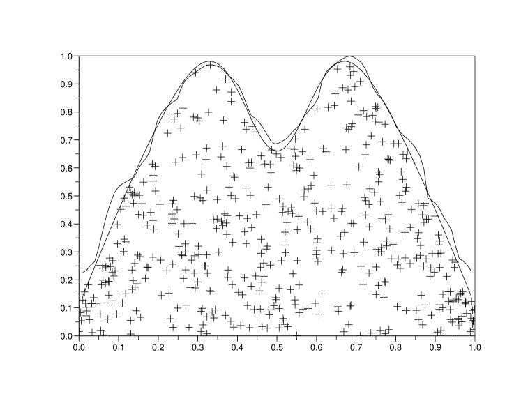
(a) Best situation

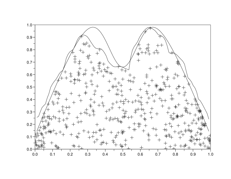
(b) Worst situation

Figure 1: The frontier $g$ (continuous line) and its estimation (dashed line). The sample size is $n=500$, $X$ is uniformly distributed on $[0,1]$ and $\gamma=1$.

Results are depicted on Figure 1–3, where the best situation (i.e. the estimation corresponding to the smallest $L_{1}$ error) and the worst situation (i.e. the estimation corresponding to the largest $L_{1}$ error) are represented. Worst situations are obtained when no points were simulated at the upper boundary of the support. To overcome this problem, the normalizing constant $(p+1)$ in (1) could be modified as in [13], Section 6 to deal with some particular parametric models of $Y$ given $X=x$.

Appendix I: Conditional bias of $\widehat{r}_{n}\left(x\right)$

In this appendix, we provide a proof of Proposition 2. From $\left(\ref{1-1}\right)$, we have

$$\mathbb{E}\left(\frac{\widehat{r}_{n}\left(x\right)}{r_{n}\left(x\right)}-1/\mathcal{X}\right)=g^{-p}\left(x\right)e_{1}^{t}\mathbf{S}_{n}^{-1}\mathbf{X}^{t}\mathbf{W}\left[\mathbb{E}\left(\mathcal{Z}/\mathcal{X}\right)-\mathbf{X\beta}\right],$$

where the term $\mathbb{E}\left(\mathcal{Z}/\mathcal{X}\right)-\mathbf{X\beta}$ can be rewritten as

$$\left(r_{n}\left(X_{1}\right)-\sum_{j=0}^{k}\beta_{j}\left(X_{1}-x\right)^{j},...,~{}r_{n}\left(X_{n}\right)-\sum_{j=0}^{k}\beta_{j}\left(X_{n}-x\right)^{j}\right).$$

Taylor-Lagrange formula with $\beta_{j}=\frac{1}{j!}\frac{\partial^{j}g^{p}}{\partial x^{j}}\left(x\right)$ and $0<\theta<1$ yields

$$g^{p}\left(u\right)=\sum_{j=0}^{k}\beta_{j}\left(u-x\right)^{j}+\left(u-x\right)^{k+1}\frac{1}{k+1!}\frac{\partial^{k+1}g^{p}}{\partial x^{k+1}}\left(x+\theta\left(u-x\right)\right),$$

so that, we can derive, for $0<\theta_{i}<1$ depending on $X_{i}$, the following expansion

$$r_{n}\left(X_{i}\right)-\sum_{j=0}^{k}\beta_{j}\left(X_{i}-x\right)^{j}=\left(X_{i}-x\right)^{k+1}\frac{1}{k+1!}\frac{\partial^{k+1}g^{p}}{\partial x^{k+1}}\left(x+\theta_{i}\left(X_{i}-x\right)\right).$$

Since $K$ has a bounded support, we have $K_{h}\left(X_{i}-x\right)=0$ for $\left|X_{i}-x\right|>h$. If $\left|X_{i}-x\right|\leq h$ and $0<\theta_{i}<1$, under the conditions $h\rightarrow 0$ and $ph\rightarrow 0$, Lemma 3 yields

$$\left(X_{i}-x\right)^{j}K_{h}\left(X_{i}-x\right)\frac{\partial^{k+1}g^{p}}{\partial x^{k+1}}\left(x+\theta_{i}\left(X_{i}-x\right)\right)$$

$$=\left(X_{i}-x\right)^{j}K_{h}\left(X_{i}-x\right)\left[\frac{\partial^{k+1}g^{p}}{\partial x^{k+1}}\left(x\right)+\sum_{j=1}^{k+1}p^{j}g^{p-j}\left(x\right)o\left(1\right)\right].$$

Thus, recalling that $S_{n,j}=\sum_{i=1}^{n}\left(X_{i}-x\right)^{j}K_{h}\left(X_{i}-x\right)$ and $\beta_{j}=\frac{1}{j!}\frac{\partial^{j}g^{p}}{\partial x^{j}}\left(x\right)$, the $(k+1)$-dimensional vector $\mathbf{X}^{t}\mathbf{W}\left(\mathbb{E}\left(\mathcal{Z}/\mathcal{X}\right)-\mathbf{X\beta}\right)$ can be rewritten as

$$\left[\sum_{i=1}^{n}\frac{\left(X_{i}-x\right)^{k+j}}{k+1!}K_{h}\left(X_{i}-x\right)\frac{\partial^{k+1}g^{p}}{\partial x^{k+1}}\left(x+\theta_{i}\left(X_{i}-x\right)\right)\right]_{j=1,...,k+1}$$

$$=\left[\beta_{k+1}S_{n,k+j}+\frac{1}{k+1!}S_{n,k+j+1}\sum_{j=1}^{k+1}p^{j}g^{p-j}\left(x\right)o\left(1\right)\right]_{j=1,...,k+1}.$$

Introducing the vector $c_{n}=\left(S_{n,k+1},...,S_{n,2k+1}\right)^{t}$, we obtain

$$\mathbf{X}^{t}\mathbf{W}\left(\mathbb{E}\left(\mathcal{Z}/\mathcal{X}\right)-\mathbf{X\beta}\right)=\beta_{k+1}c_{n}+\frac{1}{k+1!}c_{n}\sum_{j=1}^{k+1}p^{j}g^{p-j}\left(x\right)o\left(1\right),$$

and, returning to the bias of $\widehat{r}_{n}\left(x\right)$,

$$\mathbb{E}\left(\frac{\widehat{r}_{n}\left(x\right)}{r_{n}\left(x\right)}-1/\mathcal{X}\right)=g^{-p}\left(x\right)\beta_{k+1}e_{1}^{t}\mathbf{S}_{n}^{-1}c_{n}+\frac{1}{k+1!}e_{1}^{t}\mathbf{S}_{n}^{-1}c_{n}\sum_{j=1}^{k+1}p^{j}g^{-j}\left(x\right)o\left(1\right).$$ (11)

Recalling that $\mathbf{S}_{n}=nf\left(x\right)\mathbf{H}\mathbf{SH}\left[1+o_{p}\left(1\right)\right]$ with $\mathbf{H}=diag(1,h,\dots,h^{k})$, we have

$$\mathbf{S}_{n}^{-1}=\frac{1}{nf\left(x\right)}\mathbf{H}^{-1}\mathbf{S}^{-1}\mathbf{H}^{-1}\left[1+o_{p}\left(1\right)\right].$$

Besides, introducing the vector $c=\left(\mu_{k+1},...,\mu_{2k+1}\right)$, the asymptotic expression of $S_{n,j}$ established in Proposition 1 entails

$$c_{n}=nh^{k+1}f\left(x\right)\mathbf{H}c\left[1+o_{p}\left(1\right)\right].$$

Let us first focus on the first term of the bias expansion (11):

$$g^{-p}\left(x\right)e_{1}^{t}\mathbf{S}_{n}^{-1}\beta_{k+1}c_{n} =g^{-p}\left(x\right)\frac{1}{nf\left(x\right)}\beta_{k+1}nh^{k+1}f\left(x\right)e_{1}^{t}\mathbf{H}^{-1}\mathbf{S}^{-1}\mathbf{H}^{-1}\mathbf{H}c\left[1+o_{p}\left(1\right)\right]$$

$$=g^{-p}\left(x\right)h^{k+1}\beta_{k+1}e_{1}^{t}\mathbf{S}^{-1}c\left[1+o_{p}\left(1\right)\right],$$

and using the expression of $\frac{\partial^{k}g^{p}}{\partial x^{k}}$ in $\left(\ref{4-1}\right)$, we have

$$g^{-p}\left(x\right)\beta_{k+1}=\sum_{j=1}^{k+1}\frac{p!}{\left(p-j\right)!}g^{-j}\left(x\right)\phi_{\begin{subarray}{c}j\\ \end{subarray}}\left(x\right)=O\left(p^{k+1}\right),$$

leading to

$$g^{-p}\left(x\right)e_{1}^{t}\mathbf{S}_{n}^{-1}\beta_{k+1}c_{n}=e_{1}^{t}\mathbf{S}^{-1}cO_{p}\left(\left(hp\right)^{k+1}\right)=O_{p}\left(\left(hp\right)^{k+1}\right).$$ (12)

Let us now consider the second term in (11):

$$\frac{1}{k+1!}e_{1}^{t}\mathbf{S}_{n}^{-1}c_{n}\sum_{j=1}^{k+1}p^{j}g^{-j}\left(x\right)o\left(1\right) =e_{1}^{t}\mathbf{S}_{n}^{-1}c_{n}p^{k+1}o\left(1\right)$$

$$=\frac{1}{nf\left(x\right)}e_{1}^{t}\mathbf{S}^{-1}\mathbf{H}^{-1}c_{n}p^{k+1}o_{p}\left(1\right)$$

Expanding $\mathbf{H}^{-1}c_{n}$ we have

$$\mathbf{H}^{-1}c_{n}=\mathbf{H}^{-1}nh^{k+1}f\left(x\right)\mathbf{H}c\left[1+o_{p}\left(1\right)\right]=nh^{k+1}f\left(x\right)c\left[1+o_{p}\left(1\right)\right],$$

which entails

$$\frac{1}{nf\left(x\right)}e_{1}^{t}\mathbf{S}^{-1}\mathbf{H}^{-1}c_{n}p^{k+1}o_{p}\left(1\right)=e_{1}^{t}\mathbf{S}^{-1}co_{p}\left(\left(hp\right)^{k+1}\right)=o_{p}\left(\left(hp\right)^{k+1}\right).$$ (13)

Collecting (12) and (13), we obtain the announced result

$$\mathbb{E}\left(\frac{\widehat{r}_{n}\left(x\right)}{r_{n}\left(x\right)}-1/\mathcal{X}\right)=O_{p}\left(\left(hp\right)^{k+1}\right).$$

Appendix II: Auxiliary results

We first quote a Bernstein-Fréchet inequality adapted to our framework.

Lemma 1

Let $X_{1},...,X_{n}$ independent centered random variables such that for each positive integers $i$ and $k$, and for some positive constant $C$, we have

$$\mathbb{E}\left|X_{i}\right|^{k}\leq k!C^{k-2}\mathbb{E}X_{i}^{2}.$$ (14)

Then, for every $\varepsilon>0$, we have

$$\mathbb{P}\left(\left|\sum_{i=1}^{n}X_{i}\right|>\varepsilon\sqrt{\sum_{i=1}^{n}\mathbb{E}X_{i}^{2}}\right)\leq 2\exp\left\{-\frac{\varepsilon^{2}}{4+2\varepsilon C/\sqrt{\sum_{i=1}^{n}\mathbb{E}X_{i}^{2}}}\right\}.$$

The proof is standard. Note that condition (14) is verified under the boundedness assumption $\forall i\geq 1$, $\left|X_{i}\right|\leq C$. In the next lemma, an asymptotic expansion of the estimated regression function $\widehat{r}_{n}\left(x\right)=e_{1}^{t}\mathbf{S}_{n}^{-1}X^{t}\mathbf{W}\mathcal{Z}$ is introduced.

Lemma 2

The estimated regression function $\widehat{r}_{n}\left(x\right)$ can be rewritten as

$$\widehat{r}_{n}\left(x\right)=\frac{1}{nf\left(x\right)}\sum_{i=1}^{n}Z_{i}~{}K_{h}\left(X_{i}-x\right)\sum_{j=0}^{k}u_{j}\left(\frac{X_{i}-x}{h}\right)^{j}\left[1+o_{p}\left(1\right)\right],$$

where $(u_{0,}u_{1},...,u_{k})$ is the first line of the matrix $\mathbf{S}^{{}^{-1}}$.

Proof. It is known from the local polynomial fitting theory that $\widehat{r}_{n}\left(x\right)=\widehat{\beta}_{0}=e_{1}^{t}\mathbf{S}_{n}^{-1}$$x$${}^{t}\mathbf{W}\mathcal{Z}$ admits the following asymptotic expression

$$\widehat{r}_{n}\left(x\right)=\frac{1}{nhf\left(x\right)}\sum_{i=1}^{n}Z_{i}~{}K_{0}^{\ast}\left(\frac{X_{i}-x}{h}\right)\left[1+o_{p}\left(1\right)\right],$$

where

$$K_{0}^{\ast}\left(t\right)=e_{1}^{t}\mathbf{S}^{-1}\left(1,t,...,t^{k}\right)K\left(t\right)$$

is the so-called equivalent kernel, see [5]. The remaining of the proof consists in explicitly writing this equivalent kernel. It is worth noticing that $o_{p}\left(1\right)$ depends exclusively of the design $\mathcal{X}$.   

The following lemma is dedicated to the control of the local variations of the derivatives of $g^{p}$, when $p\to\infty$, on a neighborhood of size $h$.

Lemma 3

Suppose $g$ is a $C_{k+1}$ function with $k<p$. If, moreover, $ph\rightarrow 0$ and $\left|u-v\right|\leq h$, then

$$\frac{\partial^{k+1}g^{p}}{\partial x^{k+1}}\left(v\right)=\frac{\partial^{k+1}g^{p}}{\partial x^{k+1}}\left(u\right)+\sum_{j=1}^{k+1}\frac{p!}{\left(p-j\right)!}g^{p-j}\left(u\right)o(1).$$

Proof. From $\frac{\partial g^{p}}{\partial x}=pg^{p-1}\frac{\partial g}{\partial x}$ and a recurrence argument it is easily checked that

$$\frac{\partial^{k+1}g^{p}}{\partial x^{k+1}}=\sum_{j=1}^{k+1}\frac{p!}{\left(p-j\right)!}g^{p-j}\phi_{j},$$ (15)

where the $\phi_{j}$ are continuous functions. The triangular inequality entails

$$\left|g^{p-j}\left(u\right)\phi_{j}\left(u\right)-g^{p-j}\left(v\right)\phi_{j}\left(v\right)\right| \leq\left|g^{p-j}\left(u\right)\right|\left|\phi_{j}\left(u\right)-\phi_{j}\left(v\right)\right|$$

$$+\left|\phi_{j}\left(v\right)\right|\left|g^{p-j}\left(u\right)-g^{p-j}\left(v\right)\right|,$$

and, from Lemma 8, if $ph\rightarrow 0$ and $\left|u-v\right|\leq h$ we get, for sufficiently large $n$,

$$\left|g^{p-j}\left(u\right)\phi_{j}\left(u\right)-g^{p-j}\left(v\right)\phi_{j}\left(v\right)\right|\leq\left|g^{p-j}\left(u\right)\right|o(1)+c_{1}D_{j}\left|g^{p-j}\left(u\right)\right|\left(p-j\right)h,$$

where $D_{j}=\sup_{s\in\left[u,v\right]}|\phi_{j}(s)|$. Thus,

$$g^{p-j}\left(v\right)\phi_{j}\left(v\right) =g^{p-j}\left(u\right)\phi_{j}\left(u\right)+g^{p-j}\left(u\right)(O\left(ph\right)+o(1))$$

$$=g^{p-j}\left(u\right)\phi_{j}\left(u\right)+g^{p-j}\left(u\right)o(1),$$

and replacing in (15) yields

$$\frac{\partial^{k+1}g^{p}}{\partial x^{k+1}}\left(v\right) =\sum_{j=1}^{k+1}\frac{p!}{\left(p-j\right)!}g^{p-j}\left(v\right)\phi_{\begin{subarray}{c}j\\ \end{subarray}}\left(v\right)$$

$$=\sum_{j=1}^{k+1}\frac{p!}{\left(p-j\right)!}g^{p-j}\left(u\right)\phi_{\begin{subarray}{c}j\\ \end{subarray}}\left(u\right)+\sum_{j=1}^{k+1}\frac{p!}{\left(p-j\right)!}g^{p-j}\left(u\right)o(1)$$

$$=\frac{\partial^{k+1}g^{p}}{\partial x^{k+1}}\left(u\right)+\sum_{j=1}^{k+1}\frac{p!}{\left(p-j\right)!}g^{p-j}\left(u\right)o(1),$$

and the result is proved.   

Let us consider, for $i=1,\dots,n$ the random variables defined by

$$\xi_{i}=\frac{nh}{pg^{p}\left(x\right)}a\left(X_{i}\right)\left(\left(p+1\right)Y_{i}^{p}-g^{p}\left(X_{i}\right)\right).$$

The next two lemmas are preparing the application of the Bernstein-Fréchet inequality given in Lemma 1. First, it is established that the $\xi_{i}$ are bounded random variables. Second, a control of the conditional variance $\mathbb{V}\left(\sum\nolimits_{i=1}^{n}\xi_{i}/\mathcal{X}\right)$ is provided.

Lemma 4

There exists a positive constant $c_{2}$ such that $\left|\xi_{i}\right|\leq c_{2}$ for all $i=1,\dots,n$.

Proof. Since the kernel $K$ is bounded and has bounded support, it is easily seen that $a\left(X_{i}\right)=0$ if $\left|X_{i}-x\right|>h$ and that $a\left(X_{i}\right)=O\left(\frac{1}{nh}\right)$ uniformly in $i$. Noticing that $Y_{i}^{p}\leq$ $g^{p}\left(X_{i}\right)$ and using Lemma 8, we get

$$\left|\xi_{i}\right| =\frac{nh}{pg^{p}\left(x\right)}\left|a\left(X_{i}\right)\right|\left|\left(\left(p+1\right)Y_{i}^{p}-g^{p}\left(X_{i}\right)\right)\right|$$

$$\leq\frac{nh}{pg^{p}\left(x\right)}\left|a\left(X_{i}\right)\right|\left|\left(p+1\right)g^{p}\left(X_{i}\right)\right|$$ (16)

$$\leq\frac{nh}{pg^{p}\left(x\right)}\left(p+1\right)g^{p}\left(x\right)\left(1+c_{1}ph\right)O\left(\frac{1}{nh}\right)$$

$$=O\left(1\right)\left(1+O\left(ph\right)\right),$$

and the result is proved.   

Lemma 5

There exists a positive constant $c_{3}$ such that

$$\frac{nh}{p}\left/\mathbb{V}\left(\sum_{i=1}^{n}\xi_{i}/\mathcal{X}\right)\right.=c_{3}\left[1+o_{p}\left(1\right)\right],$$ (17)

or equivalently,

$$\frac{nh}{p}\left/\sqrt{\mathbb{V}\left(\sum_{i=1}^{n}\xi_{i}/\mathcal{X}\right)}\right.=\sqrt{\frac{nh}{p}}\sqrt{c_{3}}\left[1+o_{p}\left(1\right)\right].$$ (18)

Proof. Recalling that

$$\mathbb{V}\left(\left(p+1\right)Y_{i}^{p}-g^{p}\left(X_{i}\right)/\mathcal{X}\right)=\mathbb{V}\left(Z_{i}/\mathcal{X}\right)=\frac{p^{2}}{2p+1}g^{2p}\left(X_{i}\right),$$

we can write

$$\mathbb{V}\left(\sum_{i=1}^{n}\xi_{i}/\mathcal{X}\right)$$

$$=\frac{(nh)^{2}}{g^{2p}\left(x\right)}\frac{1}{2p+1}\sum_{i=1}^{n}a^{2}\left(X_{i}\right)g^{2p}\left(X_{i}\right)$$

$$=\frac{h^{2}}{g^{2p}\left(x\right)}\frac{1}{2p+1}\frac{1}{f^{2}\left(x\right)}\sum_{i=1}^{n}K_{h}^{2}\left(X_{i}-x\right)\left[\sum_{j=0}^{k}u_{j}\left(\frac{X_{i}-x}{h}\right)^{j}\right]^{2}g^{2p}\left(X_{i}\right)$$

$$=\frac{h^{2}}{g^{2p}\left(x\right)}\frac{1}{2p+1}\frac{1}{f^{2}\left(x\right)}\sum_{j,l=0}^{k}u_{j}u_{l}\sum_{i=1}^{n}K_{h}^{2}\left(X_{i}-x\right)\left(\frac{X_{i}-x}{h}\right)^{j+l}g^{2p}\left(X_{i}\right)$$

$$=\frac{h^{2}}{g^{2p}\left(x\right)}\frac{1}{2p+1}\frac{1}{f^{2}\left(x\right)}\sum_{j,l=0}^{k}u_{j}u_{l}\frac{1}{h^{j+l}}S_{n,j+l}^{\ast}.$$

Now, substituting the asymptotic expression for $S_{n,j}^{\ast}$ into the above expression yields

$$\mathbb{V}\left(\sum_{i=1}^{n}\xi_{i}/\mathcal{X}\right)=\frac{nh}{2p+1}\frac{1}{f\left(x\right)}\sum_{j,l=0}^{k}u_{j}u_{l}\nu_{j+l}\left[1+o_{p}\left(1\right)\right],$$

and the parts $\left(\ref{4-5}\right)~{}$and $\left(\ref{4-6}\right)$ of this lemma follow.   

The next two lemmas are the key tools to prove Theorem 1. Lemma 6 is mainly a consequence of the Bernstein-Fréchet inequality given in Lemma 1. Lemma 7 is dedicated to the control of the random variable $\Delta_{n}$ introduced in (5).

Lemma 6

There exists a positive constant $c_{4}$ such that for every $\varepsilon>0$,

$$\mathbb{P}\left(\left|\widehat{r}_{n}\left(x\right)-\mathbb{E}\left(\widehat{r}_{n}\left(x\right)/\mathcal{X}\right)\right|\geq\varepsilon r_{n}\left(x\right)/\mathcal{X}\right)\leq 2\exp\left\{-c_{4}\frac{nh}{p}\varepsilon^{2}\left[1+o_{p}\left(1\right)\right]\right\},$$

where the sequence $\left[1+o_{p}\left(1\right)\right]$ depends exclusively on the design $\mathcal{X}$ .

Proof. Following the asymptotic expression of $\widehat{r}_{n}\left(x\right)$ in Lemma 2, we can write

$$\mathbb{P}\left(\left|\widehat{r}_{n}\left(x\right)-\mathbb{E}\left(\widehat{r}_{n}\left(x\right)/\mathcal{X}\right)\right|\geq\varepsilon r_{n}\left(x\right)/\mathcal{X}\right)$$

$$=\mathbb{P}\left(\left|\sum_{i=1}^{n}a\left(X_{i}\right)\left(Z_{i}-\mathbb{E}\left(Z_{i}/\mathcal{X}\right)\right)\right|\left[1+o_{p}\left(1\right)\right]\geq\varepsilon r_{n}\left(x\right)/\mathcal{X}\right)$$

$$=\mathbb{P}\left(\left|\sum_{i=1}^{n}a\left(X_{i}\right)\left(\left(p+1\right)Y_{i}^{p}-g^{p}\left(X_{i}\right)\right)\right|\geq\left[1+o_{p}\left(1\right)\right]\varepsilon g^{p}\left(x\right)/\mathcal{X}\right).$$

It is worth noticing that, conditionally to $\mathcal{X}$, the sequence $o_{p}\left(1\right)$ can be seen as a deterministic sequence converging to $0$. We now introduce the bounded variables $\xi_{i}$ (see Lemma 4). In accordance with the Bernstein-Fréchet inequality given in Lemma 1, and with the expressions (17) and (18) in Lemma 5, we write

$$\mathbb{P}\left(\left|\widehat{r}_{n}\left(x\right)-\mathbb{E}\left(\widehat{r}_{n}\left(x\right)/\mathcal{X}\right)\right|\geq\varepsilon r_{n}\left(x\right)/\mathcal{X}\right)$$

$$=\mathbb{P}\left(\left|\sum\nolimits_{i=1}^{n}\xi_{i}\right|\geq\left[1+o_{p}\left(1\right)\right]\varepsilon\frac{nh}{p}/\mathcal{X}\right)$$

$$=\mathbb{P}\left(\left|\sum_{i=1}^{n}\xi_{i}\right|\geq\varepsilon\left[1+o_{p}\left(1\right)\right]\frac{nh}{p\sqrt{\mathbb{V}\left(\sum_{i=1}^{n}\xi_{i}/x\right)}}\sqrt{\mathbb{V}\left(\sum\nolimits_{i=1}^{n}\xi_{i}/x\right)}/\mathcal{X}\right)$$

$$\leq 2\exp\left\{-\frac{\left(\varepsilon\left[1+o_{p}\left(1\right)\right]\frac{nh}{p\sqrt{\mathbb{V}\left(\sum_{i=1}^{n}\xi_{i}/\mathcal{X}\right)}}\right)^{2}}{4+2\varepsilon\left[1+o_{p}\left(1\right)\right]\frac{nh}{p\sqrt{\mathbb{V}\left(\sum_{i=1}^{n}\xi_{i}/\mathcal{X}\right)}}c_{2}/\sqrt{\mathbb{V}\left(\sum_{i=1}^{n}\xi_{i}/\mathcal{X}\right)}}\right\}$$

$$=2\exp\left\{-\frac{\left(\varepsilon\sqrt{\frac{nh}{p}}\sqrt{c_{3}}\left[1+o_{p}\left(1\right)\right]\right)^{2}}{4+c_{2}\varepsilon\left[1+o_{p}\left(1\right)\right]\frac{nh}{p}/\mathbb{V}\left(\sum_{i=1}^{n}\xi_{i}/\mathcal{X}\right)}\right\}$$

$$=2\exp\left\{-\frac{\varepsilon^{2}\frac{nh}{p}c_{3}\left[1+o_{p}\left(1\right)\right]}{4+c_{2}c_{3}\varepsilon\left[1+o_{p}\left(1\right)\right]}\right\}$$

$$\leq 2\exp\left\{-c_{4}\frac{nh}{p}\varepsilon^{2}\left[1+o_{p}\left(1\right)\right]\right\},$$

and the conclusion follows.   

Lemma 7

The random variable $\Delta_{n}$ is bounded conditionally to $\mathcal{X}$, which means that there exists a positive constant, depending on the design, $c_{5}\left(\mathcal{X}\right)$ such that $\Delta_{n}\leq c_{5}\left(\mathcal{X}\right)$.

Proof. From inequality (16), we have

$$\left|\widehat{r}_{n}\left(x\right)\right| =\left|e_{1}^{t}\mathbf{S}_{n}^{-1}\mathbf{X}^{t}\mathbf{W}\mathcal{Z}\right|$$

$$=\left|\frac{1}{nf\left(x\right)}\sum\nolimits_{i=1}^{n}K_{h}\left(X_{i}-x\right)\sum_{j=0}^{k}u_{j}\left(\frac{X_{i}-x}{h}\right)^{j}Z_{i}\right|\left[1+o_{p}\left(1\right)\right]$$

$$\leq\left(\sum_{i=1}^{n}\left|a\left(X_{i}\right)\right|\left(p+1\right)g^{p}\left(X_{i}\right)\right)\left[1+o_{p}\left(1\right)\right]$$

$$=c_{1}\frac{p}{h}g^{p}\left(x\right)\left[1+o_{p}\left(1\right)\right]\frac{1}{n}card\left\{i:\left|X_{i}-x\right|<h\right\}.$$

Then, the strong law of large numbers entails

$$\left|\widehat{r}_{n}\left(x\right)\right|\leq r_{n}\left(x\right)c_{1}\frac{p}{h}\left[\mathbb{P}\left(\left|X-x\right|<h\right)\right]\left[1+o_{p}\left(1\right)\right],$$

and from the continuity of the density $f$, we have

$$\frac{1}{2h}\mathbb{P}\left(\left|X-x\right|<h\right)=f\left(x\right)\left[1+o\left(1\right)\right].$$

Consequently,

$$\left|\frac{\widehat{r}_{n}\left(x\right)}{r_{n}\left(x\right)}\right|<2c_{1}pf\left(x\right)\left[1+o_{p}\left(1\right)\right],$$

with $o_{p}\left(1\right)$ depending on the design $\mathcal{X}$. We thus write

$$\frac{1}{p}\left|w_{n}\left(x\right)\right|=\frac{1}{p}\left|\frac{\widehat{r}_{n}\left(x\right)}{r_{n}\left(x\right)}-1\right|\leq C\left(\mathcal{X}\right),$$ (19)

where $C\left(\mathcal{X}\right)$ is a positive constant under the conditioning by $\mathcal{X}$. As an immediate consequence, we get

$$\left(1+w_{n}\left(x\right)\right)^{1/p}-1=o_{p}\left(1\right).$$ (20)

From $\left(\ref{4-2}\right)$ and $\left(\ref{4-3}\right)$ it is clear that $\Delta_{n}$ is bounded conditionally to $\mathcal{X}$.   

Finally, we quote two results from [13] (Lemma 5 and Lemma 4 respectively).

Lemma 8

If $ph\rightarrow 0$, there exists a positive constant $c_{1}$ such that

$$g^{p}\left(x\right)\leq g^{p}\left(y\right)+c_{1}g^{p}\left(y\right)ph$$

for $\left|x-y\right|\leq h$.

Lemma 9

There exists a constant $c_{6}$ such that $\left|u\right|<1/2$ entails

$$\left|\left(1+u\right)^{1/p}-1-u/p\right|\leq c_{6}u^{2}/p.$$

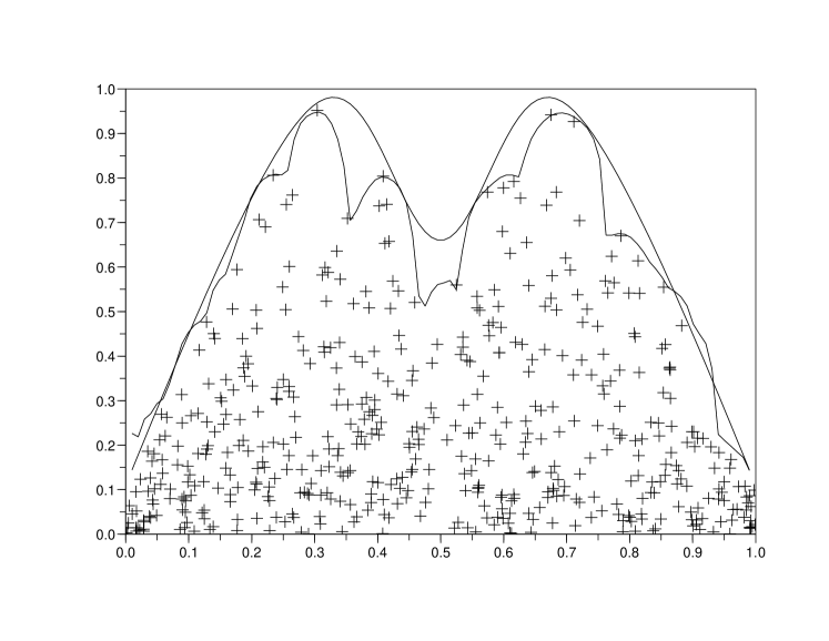
(a) Best situation

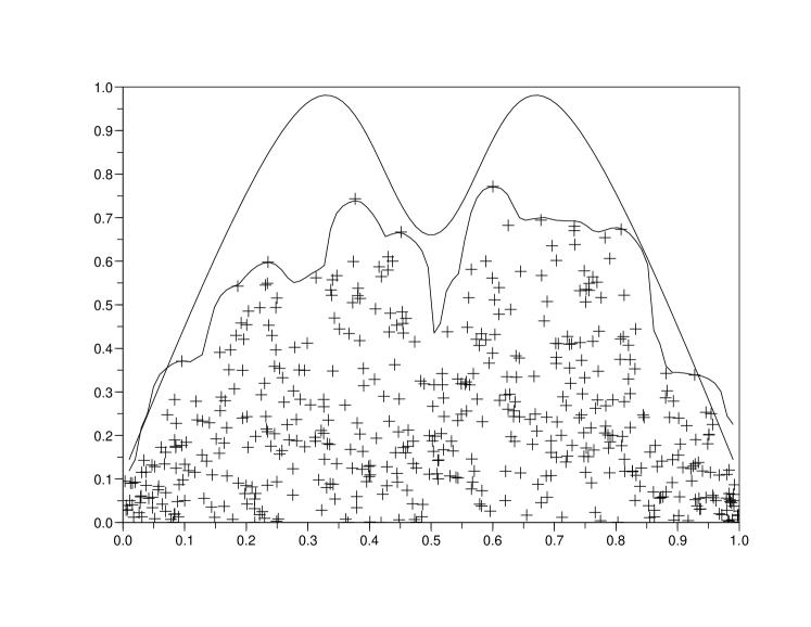
(b) Worst situation

Figure 2: The frontier $g$ (continuous line) and its estimation (dashed line). The sample size is $n=500$, $X$ is uniformly distributed on $[0,1]$ and $\gamma=2$.

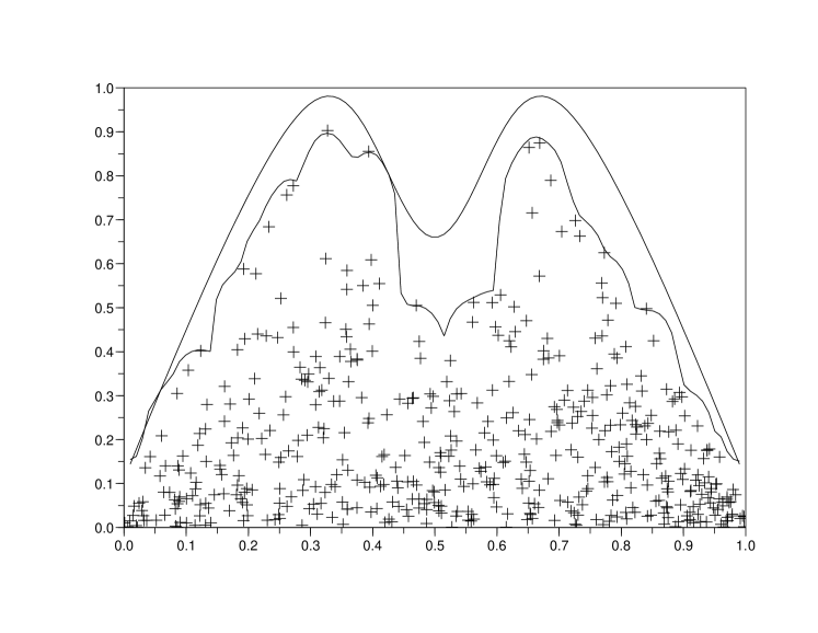
(a) Best situation

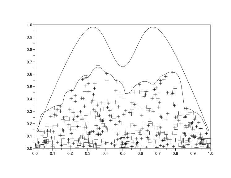
(b) Worst situation

Figure 3: The frontier $g$ (continuous line) and its estimation (dashed line). The sample size is $n=500$, $X$ is uniformly distributed on $[0,1]$ and $\gamma=3$.

References

- [1] Y. Aragon, A. Daouia and C. Thomas-Agnan. Nonparametric frontier estimation: a conditional quantile-based approach. Journal of Econometric Theory, 21(2):358–389, 2005.
- [2] C. Cazals, J.-P. Florens and L. Simar. Nonparametric frontier estimation: A robust approach. Journal of Econometrics, 106(1):1–25, 2002.
- [3] D. Deprins, L. Simar, and H. Tulkens. Measuring labor efficiency in post offices. In P. Pestieau M. Marchand and H. Tulkens, editors, The Performance of Public Enterprises: Concepts and Measurements. North Holland ed, Amsterdam, 1984.
- [4] P. Embrechts, C. Klüppelberg, and T. Mikosch. Modelling extremal events, Springer, 1997.
- [5] J. Fan and I. Gijbels, Local Polynomial Modelling and Applications, Monographs on Statistics and Applied Probability 66, Chapman & Hall, London, 1996.
- [6] M.J. Farrel. The measurement of productive efficiency. Journal of the Royal Statistical Society A, 120:253–281, 1957.
- [7] L. Gardes. Estimating the support of a Poisson process via the Faber-Shauder basis and extreme values. Publications de l’Institut de Statistique de l’Université de Paris, XXXXVI:43–72, 2002.
- [8] J. Geffroy. Sur un problème d’estimation géométrique. Publications de l’Institut de Statistique de l’Université de Paris, XIII:191–210, 1964.
- [9] I. Gijbels, E. Mammen, B. U. Park, and L. Simar. On estimation of monotone and concave frontier functions. Journal of the American Statistical Association, 94(445):220–228, 1999.
- [10] S. Girard and P. Jacob. Extreme values and Haar series estimates of point process boundaries. Scandinavian Journal of Statistics, 30(2):369–384, 2003.
- [11] S. Girard and P. Jacob. Projection estimates of point processes boundaries. Journal of Statistical Planning and Inference, 116(1):1–15, 2003.
- [12] S. Girard and P. Jacob. Extreme values and kernel estimates of point processes boundaries. ESAIM: Probability and Statistics, 8:150–168, 2004.
- [13] S. Girard and P. Jacob. Frontier estimation via kernel regression on high power-transformed data. Journal of Multivariate Analysis, 99:403–420, 2008.
- [14] S. Girard and L. Menneteau. Central limit theorems for smoothed extreme value estimates of point processes boundaries. Journal of Statistical Planning and Inference, 135(2):433–460, 2005.
- [15] P. Hall and B. U. Park. Bandwidth choice for local polynomial estimation of smooth boundaries. Journal of Multivariate Analysis, 91(2):240–261, 2004.
- [16] P. Hall, B. U. Park, and S. E. Stern. On polynomial estimators of frontiers and boundaries. Journal of Multivariate Analysis, 66(1):71–98, 1998.
- [17] W. Härdle, B. U. Park, and A. B. Tsybakov. Estimation of a non sharp support boundaries. Journal of Multivariate Analysis, 43:205–218, 1995.
- [18] P. Jacob and P. Suquet. Estimating the edge of a Poisson process by orthogonal series. Journal of Statistical Planning and Inference, 46:215–234, 1995.
- [19] K. Knight. Limiting distributions of linear programming estimators. Extremes, 4(2):87–103, 2001.
- [20] A. Korostelev, L. Simar, and A. B. Tsybakov. Efficient estimation of monotone boundaries. The Annals of Statistics, 23:476–489, 1995.
- [21] A.P. Korostelev and A.B. Tsybakov. Minimax theory of image reconstruction, volume 82 of Lecture Notes in Statistics. Springer-Verlag, New-York, 1993.
- [22] D. Ruppert and M. Wand. Multivariate locally weighted least square regression. The Annals of Statistics, 22:1343–1370, 1994.