Dynamics of a polymer chain confined in a membrane

Abstract

We present a Brownian dynamics theory with full hydrodynamics (Stokesian dynamics) for a Gaussian polymer chain embedded in a liquid membrane which is surrounded by bulk solvent and walls. The mobility tensors are derived in Fourier space for the two geometries, namely, a free membrane embedded in a bulk fluid, and a membrane sandwiched by the two walls. Within the preaveraging approximation, a new expression for the diffusion coefficient of the polymer is obtained for the free membrane geometry. We also carry out a Rouse normal mode analysis to obtain the relaxation time and the dynamical structure factor. For large polymer size, both quantities show Zimm-like behavior in the free membrane case, whereas they are Rouse-like for the sandwiched membrane geometry. We use the scaling argument to discuss the effect of excluded volume interactions on the polymer relaxation time.

1 Introduction

Integral membrane proteins play a vital role in a variety of cell functions such as solute transport, signal transduction and regulation of membrane composition alberts . Owing to finite temperatures, such proteins along with other membrane components are constantly undergoing Brownian motions. The resulting diffusive motion plays an important role in determining their transport properties. Hence the studies of diffusion constitutes an important basis for understanding the physical properties of membrane proteins, and have been an active area of focus on model systems peters-82 ; reitz-01 ; kahya-01 ; tsapis-01 ; gambin-07 as well as on living cells kucik-99 ; lippincott-01 ; vrljic-02 ; kenworthy-04 .

Although proteins consist of polymeric units of amino acids, the standard approach is to consider them as rigid disks moving in a two-dimensional (2D) liquid membrane under low-Reynolds number conditions. The diffusion coefficient of a rigid disk translating in a membrane which is embedded in a three-dimensional (3D) bulk fluid was calculated by Saffman and Delbrück (SD) saffman-75 ; saffman-76 . The obtained logarithmic size dependence is valid in the limit of small disk sizes. The SD theory was formally extended by Hughes et al. to all disk size ranges hughes-81 . In the case of large disk sizes, they showed that the diffusion coefficient is inversely proportional to its size, which is analogous to the Stoke-Einstein relation in 3D. However, it should be noted that there is no single expression of the diffusion coefficient which covers the whole disk size ranges. In a separate theoretical study, Evans and Sackmann (ES) employed a phenomenological approach to calculate the diffusion coefficient of a rigid disk moving in a membrane attached to a substrate evans-88 . The presence of a substrate in close proximity to the membrane was taken into account through a momentum decay term in the hydrodynamic equations. An extension of this work taking into account the effect of the advective terms has also been done Tserkovnyak-06 . In addition to these, diffusion of rod shaped objects on membranes levine-04 ; levine-04b or on Langmuir monolayers fischer-04 have also been theoretically analyzed.

Alternatively, the membrane protein can be regarded as a polymer chain rather than a rigid disk. In this case, the internal degrees of freedom of the polymer should be taken into account, which is the main subject of this paper. Apart from the protein analogy, hydrophobically modified polymers which adhere to the membrane could also be described using our description yang-98 . There are two theoretical works preceding the current work. One of them is a study by Muthukumar on the dynamics of a hydrophobic polymer confined in a 2D liquid membrane muthukumar-85 . In his theory, the membrane itself was treated as an isolated 2D system having an anisotropic viscosity. It was shown that the mean squared displacement of a monomer obeys a diffusive law. He also pointed out that the mode dependence of the relaxation time arises from the excluded volume effect. The second and more direct precursor to the present work is the analytical calculation of the diffusion coefficient of a polymer chain komura-95 using a 2D hydrodynamic model with momentum decay sriram-82 ; suzuki-89 ; seki-93 ; seki-07 . Since their hydrodynamic model is essentially equivalent to that used by ES, the asymptotic size dependencies of the diffusion coefficient is the same between disks and polymers; namely, logarithmic in the small size limit, and algebraic in the large size limit.

Further motivation is provided by the experiments on DNA molecules embedded on a cationic supported membrane maier-99 ; maier-00 ; maier-01 . The negative charge of the DNA molecules leads to strong adhesion with the membrane so that only the lateral motions are allowed. The measured diffusion coefficient showed a Rouse-like behavior. More recently, a similar experiment with DNA on a free standing membrane has been conducted herold-10 . Another related situation can be found in a dilute polymer solution confined between narrow slits. Based on the scaling argument, such a polymer was predicted to show a Rouse-like behavior daoud-77 ; broch-77 ; degennes-broch-77 ; tlusty-06 . In an attempt to verify these predictions, experiments on dilute solutions of DNA confined in narrow slits have shown that the exponents for conformation and chain relaxation of DNA is $2.2$ which lies between 2D and 3D behaviors lin-07 .

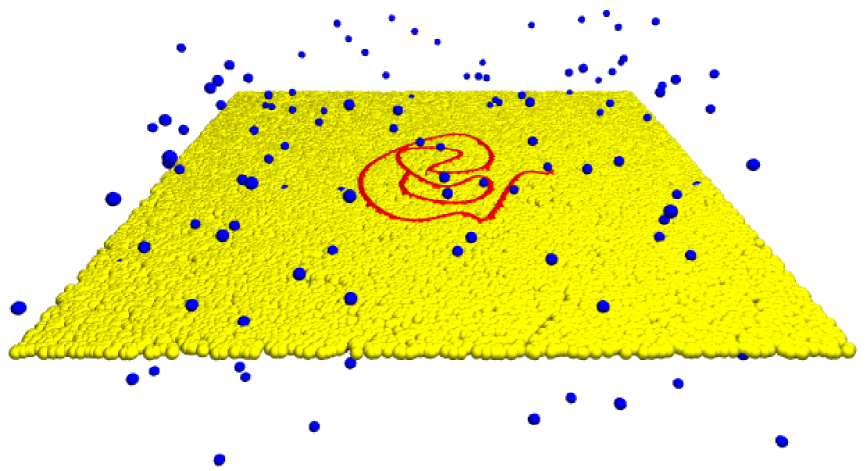
Figure 1: A transmembrane protein approximated as a polymer chain (red chain) embedded in a liquid membrane (yellow particles). The membrane itself is surrounded by solvent (blue particles). Only a few representative solvent particles are shown.

In this paper, we discuss a Brownian dynamics theory for a polymer chain confined in a membrane. As schematically presented in fig. 1, we consider a polymer chain (connected red particles) embedded in a liquid membrane (yellow particles) surrounded by a 3D bulk fluid (blue particles) and walls (not shown). We first derive the mobility tensors for the two geometries, i.e., a free membrane embedded in a bulk fluid, and a membrane sandwiched by two walls. For these two cases, we shall obtain the corresponding analytical expressions for the polymer diffusion coefficient which are valid for all sizes. We further perform a Rouse normal mode analysis to calculate the relaxation time and dynamical structure factor. For large polymer sizes, these quantities show Zimm-like behavior in the free membrane case, whereas they are Rouse-like in the presence of walls. We also use a scaling theory to discuss the effect of excluded volume interactions on the relaxation times for the two geometries. The present work demonstrates the importance of the outer environment of the membrane in determining the dynamics of a 2D polymer chain.

In the next section, we start to set up the governing equations for the membrane and the derivation of mobility tensors. With the introduction of the polymer, the general formalism of the problem is constructed in sect. 3. Sections 4 and 5 describe the results for the polymer dynamics for the free and confined membrane limiting cases, respectively. Excluded volume effects are discussed using scaling arguments in sect. 6. We finally close with several discussions in sect. 7.

2 Membrane hydrodynamics

Before introducing the polymer, we first establish the governing equations for the membrane and its surrounding environment. The aim of this section is to derive the membrane mobility tensors which will be used in the later sections for the polymer equations of motion. The present calculation closely follows the formulation by Inaura and Fujitani inaura-08 . However we consider a more general situation which will be described below. The details of the calculation are relegated to appendix A.

As shown in fig. 2, we assume that the membrane is an infinite planar sheet of liquid, and its out-of-plane fluctuations are totally neglected, which is justified for typical bending rigidities of bilayers. Relaxation dynamics of membrane fluctuations near walls have been previously considered kraus-94 ; gov-04 ; sumithra-02 . The liquid membrane is embedded in a bulk fluid such as water or solvent which is bounded by hard walls. Let ${\bf v}({\bf r})$ be the 2D velocity of the membrane fluid and the 2D vector ${\bf r}=(x,y)$ represents a point in the plane of the membrane. We first assume the membrane to be incompressible

$$\nabla\cdot{\bf v}=0,$$ (1)

where $\nabla$ is a 2D differential operator. We work in the low-Reynolds number regime of the membrane hydrodynamics so that the inertial effects can be neglected. This allows us to use the 2D Stokes equation given by

$$\eta\nabla^{2}{\bf v}-\nabla p+{\bf f}_{\rm s}+\bf{F}=0,$$ (2)

where $\eta$ is the 2D membrane viscosity, $p({\bf r})$ the 2D in-plane pressure, ${\bf f}_{\rm s}({\bf r})$ the force exerted on the membrane by the surrounding fluid (“s” stands for the solvent), and ${\bf F}({\bf r})$ is any other force acting on the membrane such as that due to a polymer chain introduced in sect. 3.

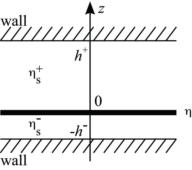
Figure 2: Schematic picture showing a planar liquid membrane having 2D viscosity $\eta$ located at $z=0$. It is sandwiched by a solvent of 3D viscosity $\eta_{\rm s}^{\pm}$. Two impenetrable walls are located at $z=\pm h^{\pm}$ bounding the solvent.

As presented in fig. 2, the membrane is fixed in the $xy$-plane at $z=0$. The upper ($z>0$) and the lower ($z<0$) fluid regions are denoted by $``+"$ and $``-"$, respectively. The velocities and pressures in these regions are written as ${\bf v}^{\pm}({\bf r},z)$ and $p^{\pm}({\bf r},z)$, respectively. Since the 3D viscosity of the upper and the lower solvent can be different, we denote them as $\eta_{\rm s}^{\pm}$ respectively. Consider the situation in which impenetrable walls are located at $z=\pm h^{\pm}$, where $h^{+}$ and $h^{-}$ can be different in general. We note that this point differs from ref. inaura-08 . Similar to the liquid membrane, the solvent in both regions are taken to be incompressible

$$\tilde{\nabla}\cdot{\bf v}^{\pm}=0,$$ (3)

where $\tilde{\nabla}$ represents a 3D differential operator. We also neglect the solvent inertia and hence the solvent obeys the 3D Stokes equations

$$\eta_{\rm s}^{\pm}\tilde{\nabla}^{2}{\bf v}^{\pm}-\tilde{\nabla}p^{\pm}=0.$$ (4)

The presence of the surrounding solvent is important because it exerts force on the liquid membrane. This force, indicated as ${\bf f}_{\rm s}$ in eq. (2), is given by the projection of $({\bm{\sigma}}^{+}-{\bm{\sigma}}^{-})_{z=0}\cdot\hat{{\bf e}}_{z}$ on the $xy$-plane. Here $\hat{{\bf e}}_{z}$ is the unit vector along the $z$-axis, and ${\bm{\sigma}}^{\pm}$ are the stress tensors due to the solvent

$${\bm{\sigma}}^{\pm}=-p^{\pm}{\bf I}+\eta_{\rm s}^{\pm}[\tilde{\nabla}{\bf v}^{\pm}+(\tilde{\nabla}{\bf v}^{\pm})^{\rm T}].$$ (5)

In the above, ${\bf I}$ is the identity tensor and the superscript “T” indicates the transpose.

Using the stick boundary conditions at $z=0$ and $z=\pm h^{\pm}$, we solve the hydrodynamic equations (3) and (4) to obtain ${\bf f}_{\rm s}$. Then we calculate the membrane velocity from eq. (2) as

$${\bf v}[{\bf k}]={{\bf G}}[{\bf k}]\cdot{\bf F}[{\bf k}],$$ (6)

where ${\bf v}[{\bf k}]$ and ${\bf F}[{\bf k}]$ are the Fourier components of ${\bf v}({\bf r})$ and ${\bf F}({\bf r})$ defined by

$${\bf v}({\bf r})=\int\frac{{\rm d}^{2}k}{(2\pi)^{2}}{\bf v}[{\bf k}]\exp(i{\bf k}\cdot{\bf r}),$$ (7)

and

$${\bf F}({\bf r})=\int\frac{{\rm d}^{2}k}{(2\pi)^{2}}{\bf F}[{\bf k}]\exp(i{\bf k}\cdot{\bf r}),$$ (8)

respectively, and ${\bf k}=(k_{x},k_{y})$. After some calculations (see appendix A for the details), one can show that the mobility tensor ${\bf G}[{\bf k}]$ in Fourier space is given by

$$G_{\alpha\beta}[{\bf k}]= \frac{1}{\eta k^{2}+k[\eta_{\rm s}^{+}\coth(kh^{+})+\eta_{\rm s}^{-}\coth(kh^{-})]}$$

$$\times\left(\delta_{\alpha\beta}-\frac{k_{\alpha}k_{\beta}}{k^{2}}\right),$$ (9)

with $\alpha,\beta=x,y$ and $k=|{\bf k}|$. As in ref. inaura-08 , we mainly consider (except in sect. 7) the case when the two walls are located at equal distances from the membrane, i.e., $h^{+}=h^{-}=h$. Then the above mobility tensor becomes

$$G_{\alpha\beta}[{\bf k}]=\frac{1}{\eta[k^{2}+\nu k\coth(kh)]}\left(\delta_{\alpha\beta}-\frac{k_{\alpha}k_{\beta}}{k^{2}}\right),$$ (10)

where $\nu\equiv 2\eta_{\rm s}/\eta$ with $\eta_{\rm s}=(\eta_{\rm s}^{+}+\eta_{\rm s}^{-})/2$. An almost equivalent expression to eq. (10) has also been derived for Langmuir monolayers in which there is only one wall or a substrate fischer-04 ; lubensky-96 . In the following, we discuss the two limiting situations of eq. (10).

Saffman and Delbrück (SD) investigated the case when the two walls are located infinitely away from the membrane saffman-75 ; saffman-76 . This is called as the free membrane case and all the related physical quantities are denoted by the superscript “SD”. Taking the limit of $kh\gg 1$ in eq. (10), the mobility tensor becomes inaura-08 ; oppenheimer-09 ; oppenheimer-10

$$G^{\rm SD}_{\alpha\beta}[{\bf k}]=\frac{1}{\eta(k^{2}+\nu k)}\left(\delta_{\alpha\beta}-\frac{k_{\alpha}k_{\beta}}{k^{2}}\right).$$ (11)

Notice that the length $\nu^{-1}$ is called the SD hydrodynamic screening length. The real space expression of this mobility tensor is obtained by the Fourier transform of eq. (11)

$${\bf G}({\bf r})=\int\frac{{\rm d}^{2}k}{(2\pi)^{2}}{\bf G}[{\bf k}]\exp(i{\bf k}\cdot{\bf r}).$$ (12)

Performing the calculations presented in appendix B, we obtain fischer-04 ; oppenheimer-09 ; oppenheimer-10

$$G^{\rm SD}_{\alpha\beta}({\bf r})= \frac{1}{4\eta}\left[{\bf H}_{0}(\nu r)-Y_{0}(\nu r)+\frac{2}{\pi\nu^{2}r^{2}}\right.$$

$$\left.-\frac{{\bf H}_{1}(\nu r)}{\nu r}+\frac{Y_{1}(\nu r)}{\nu r}\right]\delta_{\alpha\beta}$$

$$+ \frac{1}{4\eta}\left[-\frac{4}{\pi\nu^{2}r^{2}}+\frac{2{\bf H}_{1}(\nu r)}{\nu r}\right.$$

$$\left.-\frac{2Y_{1}(\nu r)}{\nu r}-{\bf H}_{0}(\nu r)+Y_{0}(\nu r)\right]\frac{r_{\alpha}r_{\beta}}{r^{2}},$$ (13)

where $r=|{\bf r}|$. In the above, ${\bf H}_{n}(z)$ are the Struve functions and $Y_{n}(z)$ are the Neumann functions or the Bessel functions of the second kind.

In the opposite $kh\ll 1$ limit, the membrane is confined between the two walls. Since such a limiting case was considered by Evans and Sackmann (ES) evans-88 , we denote all the physical quantities for this situation with the superscript “ES”. In this case, eq. (10) takes the following form

$$G^{\rm ES}_{\alpha\beta}[{\bf k}]=\frac{1}{\eta(k^{2}+\kappa^{2})}\left(\delta_{\alpha\beta}-\frac{k_{\alpha}k_{\beta}}{k^{2}}\right),$$ (14)

where $\kappa\equiv(\nu/h)^{1/2}$. This new length scale $\kappa^{-1}$ is the ES hydrodynamic screening length. We note that $\kappa^{-1}$ is the geometric mean of $\nu^{-1}$ and $h$ stone-98 . The above ES mobility tensor was previously used in a phenomenological membrane hydrodynamic model komura-95 ; seki-93 ; seki-07 ; oppenheimer-10 ; sanoop-drag-10 . Following the calculations in appendix B, the real space representation of the ES mobility tensor becomes

$$G^{\rm ES}_{\alpha\beta}({\bf r}) =\frac{1}{2\pi\eta}\left[K_{0}(\kappa r)+\frac{K_{1}(\kappa r)}{\kappa r}-\frac{1}{\kappa^{2}r^{2}}\right]\delta_{\alpha\beta}$$

$$+\frac{1}{2\pi\eta}\left[-K_{0}(\kappa r)-\frac{2K_{1}(\kappa r)}{\kappa r}+\frac{2}{\kappa^{2}r^{2}}\right]\frac{r_{\alpha}r_{\beta}}{r^{2}},$$ (15)

where $K_{n}(z)$ are the modified Bessel functions of the second kind. We use either eq. (11) or eq. (14) in our subsequent calculations with a polymer.

Strictly speaking, eqs. (13) and (15) should have been obtained by taking the limits of $\nu h\gg 1$ and $\nu h\ll 1$, respectively, after the integration of eq. (10) over ${\bf k}$. However the inverse Fourier transform of eq. (10) is nontrivial. The present approach serves our purpose and the rigorous derivation will be given in a separate publication.

3 Dynamics of a 2D Gaussian polymer chain embedded in a membrane

We are now ready to introduce a polymer into the membrane. For simplicity, we first work with a Gaussian polymer chain whose conformation is given by a set of $N$ position vectors denoted as $\{{\bf R}_{n}\}=({\bf R}_{1},\ldots,{\bf R}_{N})$ embedded in the 2D membrane. The excluded volume effects will be discussed later in sect. 6. It is implicitly assumed that the polymer relaxation time is much longer than that for the typical hydrodynamic disturbances so that the membrane can be effectively considered as a 2D liquid. If the polymer consists of monomers which exert a set of point forces ${\bf f}_{n}$ acting at ${\bf R}_{n}$, the external force due to the polymer ${\bf F}({\bf r})$ in eq. (2) can be written as

$${\bf F}({\bf r})=\sum_{n}{\bf f}_{n}\,\delta({\bf r}-{\bf R}_{n}).$$ (16)

In writing this expression, we have assumed that the superposition principle holds. With the use of the mobility tensor obtained in the previous section, eq. (2) can be formally solved as

$${\bf v}({\bf r})=\sum_{n}{\bf G}({\bf r}-{\bf R}_{n})\cdot{\bf f}_{n}.$$ (17)

Since monomers move with the same velocity as the membrane, their velocities are given by

$$\frac{\partial{\bf R}_{n}(t)}{\partial t}={\bf v}({\bf R}_{n})=\sum_{m}{\bf G}_{nm}\cdot{\bf f}_{m},$$ (18)

where we have used the notation ${\bf G}_{nm}\equiv{\bf G}({\bf R}_{n}-{\bf R}_{m})$.

The Langevin equation for a polymer chain embedded in a membrane is written as ermak-78 ; doi-edwards

$$\frac{\partial{\bf R}_{n}(t)}{\partial t} =\sum_{m}{\bf G}_{nm}\cdot\left(-\frac{\partial U}{\partial{\bf R}_{m}}+{\bm{\zeta}}_{m}(t)\right)$$

$$+\frac{k_{\rm B}T}{2}\sum_{m}\frac{\partial}{\partial{\bf R}_{m}}\cdot{\bf G}_{nm},$$ (19)

where ${\bm{\zeta}}_{m}(t)$ is the Gaussian random force acting at ${\bf R}_{m}$, $k_{\rm B}$ the Boltzmann constant, $T$ the temperature. The potential energy of the 2D polymer has the form

$$U=\frac{k_{\rm B}T}{b^{2}}\sum_{n=2}^{N}({\bf R}_{n}-{\bf R}_{n-1})^{2},$$ (20)

where $b$ is the Kuhn length. It can be shown that the mobility tensors eqs. (13) and (15) satisfy

$$\frac{\partial}{\partial{\bf R}_{m}}\cdot{\bf G}_{nm}=0.$$ (21)

Substituting eq. (20) into eq. (19) and using eq. (21), we have

$$\frac{\partial{\bf R}_{n}(t)}{\partial t}=\sum_{m}{\bf G}_{nm}\cdot\left(\frac{2k_{\rm B}T}{b^{2}}\frac{\partial^{2}{\bf R}_{m}(t)}{\partial m^{2}}+{\bm{\zeta}}_{m}(t)\right).$$ (22)

Due to the hydrodynamic coupling between different parts of the polymer, the above equation is non-linear and difficult to solve analytically. In order to overcome this difficulty, we employ the preaveraging approximation which has been successfully used for a polymer in 3D solvent doi-edwards ; zimm-56 . Assuming that the polymer is close to its equilibrium, we replace ${\bf G}_{nm}$ by its equilibrium value $\langle{\bf G}_{nm}\rangle$ such that

$$\langle{\bf G}_{nm}\rangle=\int{\rm d}\{{\bf R}_{n}\}\,{\bf G}_{nm}{\rm\Psi}(\{{\bf R}_{n}\})$$

$$=\int_{0}^{\infty}{\rm d}r\,2\pi r\frac{1}{\pi|n-m|b^{2}}\exp\left(-\frac{r^{2}}{|n-m|b^{2}}\right){\bf G}_{nm}(r)$$

$$=g(n-m){\bf I},$$ (23)

where ${\rm\Psi}(\{{\bf R}_{n}\})$ is the 2D Gaussian distribution function. Within this approximation, eq. (22) can be simplified as

$$\frac{\partial{\bf R}_{n}(t)}{\partial t}=\sum_{m}g(n-m)\left(\frac{2k_{\rm B}T}{b^{2}}\frac{\partial^{2}{\bf R}_{m}(t)}{\partial m^{2}}+{\bm{\zeta}}_{m}(t)\right).$$ (24)

The above equation can be rewritten in terms of the Rouse normal coordinates defined by doi-edwards

$${\bf X}_{p}(t)=\frac{1}{N}\int_{0}^{N}{\rm d}n\cos\left(\frac{p\pi n}{N}\right){\bf R}_{n}(t),$$ (25)

as

$$\frac{\partial{\bf X}_{p}(t)}{\partial t}=\sum_{q}g_{pq}[-k_{q}{\bf X}_{q}(t)+{\bm{\zeta}}_{q}(t)],$$ (26)

with

$$k_{p}=\frac{4\pi^{2}k_{\rm B}T}{Nb^{2}}p^{2}.$$ (27)

Here $p,q=0,1,2,\ldots$ and $g_{pq}$ is the mobility tensor in terms of the normal coordinates:

$$g_{pq}=\int_{0}^{N}\frac{{\rm d}n}{N}\int_{0}^{N}\frac{{\rm d}m}{N}\cos\left(\frac{p\pi n}{N}\right)\cos\left(\frac{q\pi m}{N}\right)g(n-m).$$ (28)

If one neglects the contribution from the off-diagonal components of $g_{pq}$, we finally obtain

$$\frac{\partial{\bf X}_{p}(t)}{\partial t}=g_{p}\left[-k_{p}{\bf X}_{p}(t)+{\bm{\zeta}}_{p}(t)\right],$$ (29)

with the definition $g_{p}\equiv g_{pp}$. The Gaussian random forces ${\bm{\zeta}}_{p}(t)$ satisfy the following conditions

$$\langle\zeta_{p\alpha}(t)\rangle=0,$$ (30)

$$\langle\zeta_{p\alpha}(t)\zeta_{q\beta}(t^{\prime})\rangle=2\delta_{pq}\delta_{\alpha\beta}(g_{p})^{-1}k_{\rm B}T\delta(t-t^{\prime}).$$ (31)

Therefore the relaxation time of a polymer in terms of the Rouse modes is given by

$$\tau_{p}=\frac{1}{g_{p}k_{p}}.$$ (32)

Furthermore, the polymer diffusion coefficient can be calculated according to the following equation

$$D=k_{\rm B}Tg_{0}=k_{\rm B}T\int_{0}^{N}\frac{{\rm d}n}{N}\int_{0}^{N}\frac{{\rm d}m}{N}\,g(n-m).$$ (33)

Another useful quantity that we calculate is the dynamic structure factor defined by

$$S({\bf k},t)=\frac{1}{N}\sum_{n,m}\langle\exp[i{\bf k}\cdot({\bf R}_{n}(t)-{\bf R}_{m}(0))]\rangle.$$ (34)

Since ${\bf R}_{n}(t)-{\bf R}_{m}(0)$ is a linear function of ${\bm{\zeta}}_{n}(t)$ obeying the Gaussian distribution, the distribution of ${\bf R}_{n}(t)-{\bf R}_{m}(0)$ is also Gaussian feller . Hence we have

$$\langle\exp(i{\bf k}\cdot[{\bf R}_{n}(t)-{\bf R}_{m}(0)])\rangle$$

$$=\exp\left(-\frac{k^{2}}{4}\langle({\bf R}_{n}(t)-{\bf R}_{m}(0))^{2}\rangle\right),$$ (35)

in 2D. Denoting the center of mass by ${\bf X}_{0}$ and using the inverse relation of eq. (25)

$${\bf R}_{n}={\bf X}_{0}+2\sum_{p=1}^{\infty}{\bf X}_{p}\cos\left(\frac{p\pi n}{N}\right),$$ (36)

we can calculate the dynamical structure factor as

$$S({\bf k},t)=\frac{1}{N}\sum_{n,m}\exp\Big{[}-k^{2}Dt-\frac{1}{4}|n-m|b^{2}k^{2}$$

$$-\frac{Nb^{2}k^{2}}{\pi^{2}}\sum_{p=1}^{\infty}\frac{1}{p^{2}}\cos\left(\frac{p\pi n}{N}\right)\cos\left(\frac{p\pi m}{N}\right)[1-\exp(-t/\tau_{p})]\Big{]}.$$ (37)

This completes the general formalism of the 2D polymer dynamics confined in a liquid membrane. In the next section, we consider the free and confined membrane cases separately by using eqs. (11) or (14) for the mobility tensor.

4 Polymer dynamics: free membrane case

When the two walls in fig. 2 are located at infinite distance from the membrane, one can use the SD mobility tensor given by eq. (11). We calculate the preaveraged mobility tensor, relaxation time, diffusion coefficient and structure factor following the recipe described in the previous section.

4.1 Mobility tensor

In order to perform the preaveraging of the mobility tensor, we take the configurational average of eq. (11) by using the equilibrium probability distribution function of a Gaussian polymer in 2D:

$$\langle{\bf G}^{\rm SD}_{nm}\rangle =\left\langle\int\frac{{\rm d}^{2}k}{(2\pi)^{2}}\frac{{\mathbf{I}}-\hat{\bf k}\hat{\bf k}}{\eta(k^{2}+\nu k)}\exp[i{\bf k}\cdot({\bf R}_{n}-{\bf R}_{m})]\right\rangle,$$ (38)

where $\hat{\bf k}$ denotes a unit vector along ${\bf k}$. This leads to $\langle{\bf G}_{nm}^{\rm SD}\rangle=g^{\rm SD}(n-m){\bf I}$ with

$$g^{\rm SD}(n-m)$$

$$=\frac{1}{4\pi\eta}\int_{0}^{\infty}{\rm d}k\,\frac{k}{k^{2}+\nu k}\exp\left(-\frac{1}{4}b^{2}k^{2}|n-m|\right)$$

$$=\frac{1}{8\pi\eta}\exp\left(-\frac{1}{4}b^{2}\nu^{2}|n-m|\right)$$

$$\times\left[\pi{\rm erfi}\left(\frac{1}{2}b\nu\sqrt{|n-m|}\right)-{\rm Ei}\left(\frac{1}{4}b^{2}\nu^{2}|n-m|\right)\right],$$ (39)

where ${\rm erfi}(z)$ is the imaginary error function

$${\rm erfi}(z)=-i{\rm erf}(iz),$$ (40)

with ${\rm erf}(z)$ being the error function

$${\rm erf}(z)=\frac{2}{\sqrt{\pi}}\int_{0}^{z}{\rm d}u\,e^{-u^{2}},$$ (41)

whereas ${\rm Ei}(-z)$ is the exponential integral given by abram-stegun

$${\rm Ei}(-z)=-\int_{z}^{\infty}{\rm d}u\,\frac{e^{-u}}{u}.$$ (42)

It should be noted that the obtained $g^{\rm SD}(n-m)$ is real despite the presence of complex functions.

4.2 Relaxation time

In order to obtain the polymer relaxation time, we first substitute eq. (39) into eq. (28) to express the mobility tensor in terms of the Rouse normal coordinates

$$g^{\rm SD}_{p}=\frac{1}{\pi\eta Nb^{2}}\int_{0}^{\infty}{\rm d}k\,\frac{k^{3}}{(k^{2}+\nu k)[k^{4}+\left(4\pi p/Nb^{2}\right)^{2}]}$$

$$=\frac{1}{16\pi\eta}\frac{\pi^{2}p-\sqrt{2p}\pi^{3/2}\delta+2\ln(\pi p/\delta^{2})\delta^{2}+(\sqrt{2\pi/p})\delta^{3}}{\pi^{2}p^{2}+\delta^{4}},$$ (43)

(note that $g^{\rm SD}_{p}=g^{\rm SD}_{pp}$). In the above, we have defined the dimensionless polymer size $\delta\equiv\sqrt{N}b\nu/2$. Since the radius of gyration for the 2D Gaussian polymer is $R_{\rm g}=\sqrt{N}b/2$ doi-edwards , $\delta$ can be also written as $\delta=R_{\rm g}\nu$. Using eq. (32), the relaxation time becomes

$$\tau_{p}^{\rm SD}=\frac{4Nb^{2}\eta}{\pi k_{\rm B}T}$$

$$\times\frac{\pi^{2}p^{2}+\delta^{4}}{p^{2}[\pi^{2}p-\sqrt{2p}\pi^{3/2}\delta+2\ln(\pi p/\delta^{2})\delta^{2}+(\sqrt{2\pi/p})\delta^{3}]}.$$ (44)

This expression shows how the presence of the bulk solvent affects the relaxation time.

We consider two asymptotic limits of eq. (44). For small polymer sizes or $\delta\ll 1$, we have

$$\tau_{p}^{\rm SD}\approx\frac{4Nb^{2}\eta}{\pi k_{\rm B}T}\frac{1}{p}.$$ (45)

For large sizes, the condition $\delta\gg 1$ yields

$$\tau_{p}^{\rm SD}\approx\frac{4Nb^{2}\eta}{\pi k_{\rm B}T}\frac{\delta}{\sqrt{2\pi}p^{3/2}}.$$ (46)

It should be noticed that eq. (46) depends only on the solvent viscosity $\eta_{\rm s}$ but not on the membrane viscosity $\eta$.

Figure 3: Scaled relaxation time $\pi k_{\rm B}T\tau_{p}/4Nb^{2}\eta$ as a function of $\delta=R_{\rm g}\nu$ for free membranes (solid lines) or $\varepsilon=R_{\rm g}\kappa$ for confined membranes (dashed lines) for $p=1$ and $10$.

Figure 4: Scaled relaxation time $\pi k_{\rm B}T\tau_{p}/4Nb^{2}\eta$ as a function of $p$ for different values of $\delta=0.01,100$ (solid lines) and $\varepsilon=0.01,100$ (dashed lines). The two curves for $\delta=\varepsilon=0.01$ overlap each other and cannot be distinguished.

In fig. 3, the scaled relaxation time eq. (44) is plotted as a function of $\delta$ for $p=1$ and $10$ as solid lines. For small $\delta$, the relaxation time is independent of the polymer size, which is consistent with eq. (45). The relaxation time increases through a crossover regime towards a linear behavior as given by eq. (46). Such a crossover occurs around the region where the polymer size $R_{\rm g}$ is comparable to the SD hydrodynamic screening length $\nu^{-1}$, i.e., $\delta\sim 1$. In the limit of large $\delta$, the $p$-dependence of the relaxation time is analogous to that obtained from the Zimm model doi-edwards . The solid lines in fig. 4 show the relaxation time as a function of the Rouse normal mode $p$ for $\delta=0.01$ and $100$. These lines have slopes $-1$ and $-3/2$ for $\delta=0.01$ and $100$, respectively. These results indicate the different mode dependencies in the two limiting polymer sizes.

4.3 Diffusion coefficient

By substituting eq. (39) into eq. (33), the diffusion coefficient of the polymer can be obtained as

$$D^{\rm SD} =\frac{k_{\rm B}T}{4\pi\eta}\frac{1}{\delta^{4}}\left[(\pi\,{\rm erfi}(\delta)-{\rm Ei}(\delta^{2}))\exp(-\delta^{2})+\frac{4\sqrt{\pi}}{3}\delta^{3}\right.$$

$$+\delta^{2}-(\ln\delta^{2}+\gamma)(\delta^{2}-1)-2\sqrt{\pi}\delta\bigg{]},$$ (47)

where $\gamma=0.5772\cdots$ is Euler’s constant. This expression for the polymer diffusion coefficient is valid for all the ranges of $\delta$. Equation (47) is one of the main results of this paper.

We now discuss the asymptotic limits of eq. (47) for small and large polymer sizes. When $\delta\ll 1$, it reduces to

$$D^{\rm SD}\approx\frac{k_{\rm B}T}{4\pi\eta}\left(-\ln\delta-\frac{\gamma}{2}+\frac{3}{4}\right).$$ (48)

Such a logarithmic behavior is consistent with that of an object in a pure 2D system saffman-75 ; saffman-76 . In the opposite limit of $\delta\gg 1$, we have

$$D^{\rm SD}\approx\frac{k_{\rm B}T}{4\pi\eta}\frac{4\sqrt{\pi}}{3\delta}=\frac{k_{\rm B}T}{6\sqrt{\pi}\eta_{\rm s}R_{\rm g}}.$$ (49)

Similar to eq. (46), this expression depends only on $\eta_{\rm s}$. The obtained $1/\eta_{\rm s}R_{\rm g}$-dependence is analogous to that of an object moving in 3D fluid as well as the result by Hughes et al. hughes-81 .

Figure 5: Dimensionless diffusion coefficient $4\pi\eta D/k_{\rm B}T$ as a function of $\delta=R_{\rm g}\nu$ (solid line) or $\varepsilon=R_{\rm g}\kappa$ (dashed line).

In fig. 5, we plot the diffusion coefficient $D^{\rm SD}$ as a function of $\delta$ (solid curve). With the increase in the polymer size, there is a crossover from logarithmic to algebraic decay indicated by eqs. (48) and (49), respectively. The change in the behavior of a domain of the diffusion coefficient with the addition of solvent has also been shown through recent dissipative particle dynamics simulations on pure 2D and quasi-2D systems sanoop-bulk-10 .

4.4 Dynamic structure factor

The last quantity calculated for the free membrane geometry is the dynamical structure factor $S^{\rm SD}({\bf k},t)$ defined in eq. (34). Since the full expression is rather complicated, we derive several analytical expressions for the limiting cases. For $R_{\rm g}k\ll 1$, we have

$$S^{\rm SD}({\bf k},t)\approx N\exp(-k^{2}D^{\rm SD}t),$$ (50)

where $D^{\rm SD}$ is given by eq. (47). This is reasonable because only the center of mass motion of the polymer is captured in the small angle regime.

For $R_{\rm g}k\gg 1$, on the other hand, we only consider the time region $t\ll\tau_{p}^{\rm SD}$ because $S^{\rm SD}({\bf k},t)$ becomes very small for $t\gg\tau_{p}^{\rm SD}$. In this case, we have

$$S^{\rm SD}({\bf k},t)\approx\frac{1}{N}\sum_{n,m}\exp\Big{[}-\frac{1}{4}|n-m|b^{2}k^{2}-\frac{Nb^{2}k^{2}}{\pi^{2}}$$

$$\times\sum_{p=1}^{\infty}\frac{1}{p^{2}}\cos\left(\frac{p\pi n}{N}\right)\cos\left(\frac{p\pi m}{N}\right)[1-\exp(-t/\tau_{p}^{\rm SD})]\Big{]}$$

$$=\frac{8}{b^{2}k^{2}}\int_{0}^{\infty}{\rm d}u\,\exp(-u-k^{2}I_{1}(u)),$$ (51)

with

$$I_{1}(u)=\frac{Nb^{2}}{2\pi^{2}}\int_{0}^{\infty}{\rm d}p\,\frac{1}{p^{2}}\cos\left(\frac{4\pi pu}{Nb^{2}k^{2}}\right)[1-\exp(-t/\tau_{p}^{\rm SD})].$$ (52)

When $\delta\gg 1$, we can use the limiting expression for $\tau_{p}^{\rm SD}$ as obtained in eq. (46). In this case, the above expression becomes

$$S^{\rm SD}({\bf k},t)$$

$$\approx\frac{8}{b^{2}k^{2}}\int_{0}^{\infty}{\rm d}u\,\exp\left[-u-(\Gamma^{\rm SD}t)^{2/3}w_{1}((\Gamma^{\rm SD}t)^{-2/3}u)\right],$$ (53)

with the decay rate

$$\Gamma^{\rm SD}=\frac{k_{\rm B}T\sqrt{N}bk^{3}}{16\eta\delta}=\frac{k_{\rm B}Tk^{3}}{8\eta\nu},$$ (54)

and

$$w_{1}(u)=\frac{2}{\pi}\int_{0}^{\infty}{\rm d}x\,\frac{\cos(xu)}{x^{2}}[1-\exp(-x^{3/2}/\sqrt{2})].$$ (55)

Notice the $k^{3}$-dependence of the decay rate. For $\Gamma^{\rm SD}t\gg 1$, the above expression is further simplified to

$$S^{\rm SD}({\bf k},t)\approx S^{\rm SD}({\bf k},0)\exp(-1.35(\Gamma^{\rm SD}t)^{2/3}),$$ (56)

since $w_{1}(0)=\Gamma(1/3)\approx 1.35$. This expression is valid in the limit of large polymer sizes such that $R_{\rm g}k\gg 1$ and $\delta\gg 1$. Large wave vectors (probing the internal motion of the polymer) and hydrodynamic screening lengths (high solvent viscosity) will also lead to the same expression. The applicable time window for eq. (56) is $1/\Gamma^{\rm SD}\ll t\ll\tau_{p}^{\rm SD}$. These expressions for large $\delta$ are analogous to that obtained from the Zimm model doi-edwards in the $R_{\rm g}k\gg 1$ regime for polymer in 3D.

5 Polymer dynamics: confined membrane case

When the thickness of the solvent layers is very small, the membrane is now almost confined by the two walls. However, there is a thin lubricating layer between the membrane and the walls so that $h\neq 0$. In this case, we use the ES mobility tensor given by eq. (14). Several quantities for this case are obtained below.

5.1 Mobility tensor

By using eq. (14), the preaveraged mobility tensor is calculated from

$$\langle{\bf G}^{\rm ES}_{nm}\rangle=\left\langle\int\frac{{\rm d}^{2}k}{(2\pi)^{2}}\frac{{\mathbf{I}}-\hat{\bf k}\hat{\bf k}}{\eta(k^{2}+\kappa^{2})}\exp[i{\bf k}\cdot({\bf R}_{n}-{\bf R}_{m})]\right\rangle.$$ (57)

This results in $\langle{\bf G}^{\rm ES}_{nm}\rangle=g^{\rm ES}(n-m){\bf I}$ with

$$g^{\rm ES}(n-m)$$

$$=\frac{1}{4\pi\eta}\int_{0}^{\infty}{\rm d}k\,\frac{k}{k^{2}+\kappa^{2}}\exp\left(-\frac{1}{4}b^{2}k^{2}|n-m|\right)$$

$$=-\frac{1}{8\pi\eta}\exp\left(\frac{1}{4}b^{2}\kappa^{2}|n-m|\right){\rm Ei}\left(-\frac{1}{4}b^{2}\kappa^{2}|n-m|\right),$$ (58)

which was previously derived in ref. komura-95 .

5.2 Relaxation time

The polymer relaxation time can be obtained by substituting eq. (58) into eq. (28). Then we have

$$g^{\rm ES}_{p} =\frac{1}{\pi\eta Nb^{2}}\int_{0}^{\infty}{\rm d}k\,\frac{k^{3}}{(k^{2}+\kappa^{2})[k^{4}+\left(4\pi p/Nb^{2}\right)^{2}]}$$

$$=\frac{1}{16\pi\eta}\frac{\pi^{2}p+2\varepsilon^{2}\ln(\varepsilon^{2}/(\pi p))}{\pi^{2}p^{2}+\varepsilon^{4}}.$$ (59)

In the above, we have defined the dimensionless polymer size as $\varepsilon\equiv\sqrt{N}b\kappa/2=R_{\rm g}\kappa$ which should be distinguished from $\delta$ in the previous section. Then the relaxation time can be written as

$$\tau^{\rm ES}_{p}=\frac{4Nb^{2}\eta}{\pi k_{\rm B}T}\frac{\pi^{2}p^{2}+\varepsilon^{4}}{p^{2}[\pi^{2}p+2\varepsilon^{2}\ln(\varepsilon^{2}/(\pi p))]}.$$ (60)

In the limit of $\varepsilon\ll 1$, it reduces to

$$\tau_{p}^{\rm ES}\approx\frac{4Nb^{2}\eta}{\pi k_{\rm B}T}\frac{1}{p},$$ (61)

which coincides with eq. (45). In the opposite limit of $\varepsilon\gg 1$, one gets

$$\tau_{p}^{\rm ES}\approx\frac{4Nb^{2}\eta}{\pi k_{\rm B}T}\frac{\varepsilon^{2}}{2p^{2}\ln(\varepsilon^{2}/(\pi p))}.$$ (62)

In fig. 3, we plot $\tau_{p}^{\rm ES}$ as a function of $\varepsilon$ for $p=1$ and $10$ in dashed lines. The algebraic $\varepsilon^{2}$-dependence in eq. (62) is seen for large $\varepsilon$. The dashed lines in fig. 4 are the plots of $\tau_{p}^{\rm ES}$ as a function of $p$ for $\varepsilon=0.01$ and $100$. For $\varepsilon=100$, the slope $-2$ is consistent with eq. (62) neglecting the logarithmic correction. Notice that this $p$-dependence is in contrast to that for the free membrane case given in eq. (46).

5.3 Diffusion coefficient

With the use of eq. (58), the diffusion coefficient for the confined membrane geometry is written as

$$D^{\rm ES} =\frac{k_{\rm B}T}{4\pi\eta}\frac{1}{\varepsilon^{4}}[(1+\varepsilon^{2})(2\ln\varepsilon+\gamma)-\varepsilon^{2}$$

$$-\exp(\varepsilon^{2}){\rm Ei}(-\varepsilon^{2})].$$ (63)

This equation was also obtained before komura-95 . The limiting expression for $\varepsilon\ll 1$ is

$$D^{\rm ES}\approx\frac{k_{\rm B}T}{4\pi\eta}\left(-\ln\varepsilon-\frac{\gamma}{2}+\frac{3}{4}\right),$$ (64)

which coincides with eq. (48) as long as $\varepsilon$ is replaced by $\delta$. When $\varepsilon\gg 1$, eq. (63) reduces to

$$D^{\rm ES}\approx\frac{k_{\rm B}T}{4\pi\eta}\frac{1}{\varepsilon^{2}}=\frac{k_{\rm B}Th}{8\pi\eta_{\rm s}R_{\rm g}^{2}}.$$ (65)

This $1/R_{\rm g}^{2}$-dependence is a characteristic of a system in which there is momentum loss from the membrane to the surrounding environment diamant-09b . An intuitive understanding of the large size behaviors of the diffusion coefficient in terms of the conservation principles will be described in sect. 7. The dashed line in fig. 5 shows the plot of $D^{\rm ES}$ as a function of $\varepsilon$, showing the logarithmic and algebraic behaviors as derived above.

According to the definition of $\delta$ and $\varepsilon$, one obtains $\varepsilon=\delta/\sqrt{\nu h}$. This correspondence leads to a rescaling of the $\varepsilon$-axis in figs. 3 and 5. Here the value of $\sqrt{\nu h}$ cannot be taken arbitrarily since the condition for the confined membrane is given by $\nu h\ll 1$ as explained in sect. 2.

5.4 Dynamic structure factor

The dynamic structure factor can be calculated in the same manner as before. For $R_{\rm g}k\ll 1$, we have

$$S^{\rm ES}({\bf k},t)\approx N\exp(-k^{2}D^{\rm ES}t).$$ (66)

For $R_{\rm g}k\gg 1$ and $t\ll\tau_{p}^{\rm ES}$, we get

$$S^{\rm ES}({\bf k},t)\approx\frac{8}{b^{2}k^{2}}\int_{0}^{\infty}{\rm d}u\,\exp(-u-k^{2}I_{2}(u)),$$ (67)

with

$$I_{2}(u)=\frac{Nb^{2}}{2\pi^{2}}\int_{0}^{\infty}{\rm d}p\,\frac{1}{p^{2}}\cos\left(\frac{4\pi pu}{Nb^{2}k^{2}}\right)[1-\exp(-t/\tau_{p}^{\rm ES})].$$ (68)

Considering $\varepsilon\gg 1$ and neglecting the logarithmic dependence in eq. (62), the above expression becomes

$$S^{\rm ES}({\bf k},t)$$

$$\approx\frac{8}{b^{2}k^{2}}\int_{0}^{\infty}{\rm d}u\,\exp\left[-u-(\Gamma^{\rm ES}t)^{1/2}w_{2}((\Gamma^{\rm ES}t)^{-1/2}u)\right],$$ (69)

with the decay rate

$$\Gamma^{\rm ES}=\frac{k_{\rm B}TNb^{2}k^{4}}{32\pi\eta\varepsilon^{2}}=\frac{k_{\rm B}Tk^{4}}{8\pi\eta\kappa^{2}},$$ (70)

and

$$w_{2}(u)=\frac{2}{\pi}\int_{0}^{\infty}{\rm d}x\,\frac{\cos(xu)}{x^{2}}[1-\exp(-x^{2})].$$ (71)

Note that $\Gamma^{\rm ES}$ is proportional to $k^{4}$ as for the Rouse model. For $\Gamma^{\rm ES}t\gg 1$, it can be further simplified to

$$S^{\rm ES}({\bf k},t)\approx S^{\rm ES}({\bf k},0)\exp(-1.13(\Gamma^{\rm ES}t)^{1/2}),$$ (72)

since $w_{2}(0)=2/\sqrt{\pi}\approx 1.13$. This expression is valid when $R_{\rm g}k\gg 1$ and $\varepsilon\gg 1$. The relevant time interval for this expression is $1/\Gamma^{\rm ES}\ll t\ll\tau_{p}^{\rm ES}$.

6 Excluded volume effects

So far, we have treated only a 2D Gaussian polymer chain. In this section, we briefly discuss the effects of excluded volume on the dynamical quantities. Even if the polymer is not a Gaussian chain, one can still use the preaveraging approximation for the mobility tensor. For the free membrane case, one can generally show that

$$g^{\rm SD}(n-m)=\frac{1}{8\eta}\langle{\bf H}_{0}(\nu r_{nm})-Y_{0}(\nu r_{nm})\rangle,$$ (73)

where $r_{nm}=|{\bf R}_{n}-{\bf R}_{m}|$ (see appendix B). Then the diffusion coefficient can be expressed as

$$D^{\rm SD}=\frac{k_{\rm B}T}{8\eta}\int_{0}^{N}\frac{{\rm d}n}{N}\int_{0}^{N}\frac{{\rm d}m}{N}\langle{\bf H}_{0}(\nu r_{nm})-Y_{0}(\nu r_{nm})\rangle.$$ (74)

Similarly for the confined membrane case, we find

$$D^{\rm ES}=\frac{k_{\rm B}T}{4\pi\eta}\int_{0}^{N}\frac{{\rm d}n}{N}\int_{0}^{N}\frac{{\rm d}m}{N}\langle K_{0}(\kappa r_{nm})\rangle,$$ (75)

(see eq. (B.14)). These expressions are the 2D analog of the Kirkwood formula doi-edwards . It should be emphasized that they are rigorous even in the presence of excluded volume effect.

For excluded volume chains, however, the appropriate equilibrium distribution function ${\rm\Psi}(\{{\bf R}_{n}\})$ needed to calculate averages is not known doi-edwards . Therefore, we cannot obtain rigorous forms of diffusion coefficient. Instead, we shall make use of scaling arguments to infer the effects of excluded volume interactions. Here, we limit our discussion to small and large polymer sizes. A simple argument is that the excluded volume effects lead to a rescaled polymer radius of gyration $R_{\rm g}$. Within the Flory theory, the radius of gyration scales as $R_{\rm g}\sim bN^{\nu_{\rm F}}$ using the Flory exponent $\nu_{\rm F}$. Up to a numerical factor, the diffusion coefficient in the limiting cases will still show the same size dependence as in eqs. (48), (49), (64) and (65) in which $R_{\rm g}$ is now replaced with that of excluded volume chains. In other words, we replace $N$ with $N^{2\nu_{\rm F}}$ in these equations. On the other hand, the relaxation time in the presence of the excluded volume effects can be obtained by replacing $N/p$ with $(N/p)^{2\nu_{\rm F}}$ in the Gaussian chain cases. In the small size limits, i.e, $\delta,\varepsilon\ll 1$, we have

$$\tau^{\rm SD}\sim\frac{\eta b^{2}}{k_{\rm B}T}\left(\frac{N}{p}\right)^{2\nu_{\rm F}},$$ (76)

and

$$\tau^{\rm ES}\sim\frac{\eta b^{2}}{k_{\rm B}T}\left(\frac{N}{p}\right)^{2\nu_{\rm F}}.$$ (77)

In the opposite of large polymer size limits, i.e., $\delta,\varepsilon\gg 1$, we get

$$\tau^{\rm SD}\sim\frac{\eta b^{3}\nu}{k_{\rm B}T}\left(\frac{N}{p}\right)^{3\nu_{\rm F}},$$ (78)

and

$$\tau^{\rm ES}\sim\frac{\eta b^{4}\kappa^{2}}{k_{\rm B}T}\left(\frac{N}{p}\right)^{4\nu_{\rm F}}.$$ (79)

These are the scaling predictions. Notice that the above results can also be obtained by using the relation $\tau\sim R_{\rm g}^{2}/D$ where $R_{\rm g}$ includes the excluded volume effect rubinstein-colby .

Table 1 shows the comparison between a Gaussian chain polymer ($\nu_{\rm F}=1/2$) and a chain with excluded volume interactions ($\nu_{\rm F}=3/4$) in 2D. The former Gaussian case recovers all the relations in the previous sections (see eqs. (45), (61), (46), (62)). For the chain with $\nu_{\rm F}=3/4$, the relaxation time shows a $p^{-3/2}$-dependence for both the free and confined membrane cases when $\delta,\varepsilon\ll 1$. This is consistent with the result in ref. muthukumar-85 . For $\delta\gg 1$ and $\varepsilon\gg 1$, we have $\tau^{\rm SD}\sim p^{-9/4}$ and $\tau^{\rm ES}\sim p^{-3}$, respectively. These exponents are unique for polymers confined in a membrane.

Table 1: Comparison of the relaxation times between a Gaussian polymer chain and a polymer with excluded volume interactions.

limits	ideal chain ($\nu_{\rm F}=1/2$)	real chain ($\nu_{\rm F}=3/4$)
$\delta\ll 1$	$\tau^{\rm SD}\sim p^{-1}$	$\tau^{\rm SD}\sim p^{-3/2}$
$\varepsilon\ll 1$	$\tau^{\rm ES}\sim p^{-1}$	$\tau^{\rm ES}\sim p^{-3/2}$
$\delta\gg 1$	$\tau^{\rm SD}\sim p^{-3/2}$	$\tau^{\rm SD}\sim p^{-9/4}$
$\varepsilon\gg 1$	$\tau^{\rm ES}\sim p^{-2}$	$\tau^{\rm ES}\sim p^{-3}$

7 Discussion

In this paper, we have investigated the dynamics of a Gaussian polymer chain confined in a liquid membrane taking into account the surrounding environment. For the most general geometry with the membrane, solvent and walls (see fig. 2), we have derived the mobility tensor in eq. (9). We obtained the analytical expressions for the relaxation time, diffusion coefficient and dynamic structure factor of a Gaussian chain for the two limiting cases of free and confined membranes. These quantities were calculated within the preaveraging approximation of the mobility tensor in order to avoid the non-linearity introduced by the hydrodynamic coupling. We shall summarize and discuss the results obtained in this paper.

Our theoretical analysis relies on the preaveraging approximation, which is used to decouple the polymer fluctuations from hydrodynamics. The validity of this approximation has been studied in some detail for polymers in a 3D bulk fluid, where the preaveraging approximation (Zimm model) yields results which are not very different from more sophisticated calculations doi-edwards . The response of a dilute polymer solution to an external field has also been experimentally verified to follow the predictions of the Zimm model johnson-70 . Deviations from the Zimm model have been attributed to non-Gaussian distributions, the slowness to reach asymptotic behaviors or the effect of hydrodynamic fluctuations, although a clear conclusion has not been reached stockmayer-84 . Up to now, there have not been any experimental studies of the dynamics of polymers confined to membranes, to the best of our knowledge. Experiments using a combination of Langmuir trough as well as light scattering techniques should be able to test our predictions. The success of preaveraging in three-dimensional polymer solutions encourages us to expect the same to hold for quasi-2D systems.

We first compare the relaxation times between the two cases. As seen from eqs. (45) and (61) for small polymer sizes, i.e., $\delta,\varepsilon\ll 1$, both $\tau_{p}^{\rm SD}$ and $\tau_{p}^{\rm ES}$ show exactly the same mode dependence. This is due to the fact that for polymer sizes smaller than than the hydrodynamic screening lengths ($\nu^{-1}$ or $\kappa^{-1}$), the outer environment does not affect the polymer dynamics. The behavior $\tau_{p}^{\rm SD}\sim p^{-3/2}$ for $\delta\gg 1$ (see eq. (46)) is analogous to the Zimm relaxation time of a Gaussian polymer in a 3D solvent. On the other hand, the dependence $\tau_{p}^{\rm ES}\sim p^{-2}$ for $\varepsilon\gg 1$ (see eq. (62)) is similar to the Rouse relaxation time in 3D.

One of the important results of this paper is the derivation of eq. (47) which provides the diffusion coefficient valid for all size ranges in the free membrane case. According to eqs. (48) and (64), the diffusion coefficients $D^{\rm SD}$ and $D^{\rm ES}$ show the same logarithmic dependence when $\delta,\varepsilon\ll 1$. Again this occurs when the polymer size is smaller than $\nu^{-1}$ or $\kappa^{-1}$. A crossover from logarithmic to algebraic behavior takes place when the polymer size $R_{\rm g}$ is comparable to these hydrodynamic screening lengths. Thus $\nu^{-1}$ or $\kappa^{-1}$ determines the length scale at which the outer environment surrounding the membrane becomes important. For a pure 2D system, the screening length is infinite, which causes the Stokes paradox.

When the polymer size becomes much larger than the hydrodynamic screening lengths, the interactions are no longer only through the membrane. In the free membrane case, the outer fluid plays the role of the mediator of the hydrodynamic interactions. This attributes a 3D nature to the polymer dynamics and hence the scaling $D^{\rm SD}\sim 1/\eta_{\rm s}R_{\rm g}$ is recovered (see eq. (49)). In the confined membrane case, the presence of the walls takes away the momentum from the membrane. Owing to the stick boundary condition, a linear shear velocity gradient is set up in the intervening fluid layer between the membrane and the walls leading to a momentum leakage from the membrane. As given in eq. (65), the resultant diffusion coefficient behaves as $D^{\rm ES}\sim 1/R_{\rm g}^{2}$. These asymptotic behaviors are consistent with the results of correlated diffusion obtained in ref. oppenheimer-10 .

The different large size behaviors of the diffusion coefficient can be better understood by focusing on the mobility tensors. It is essentially described as a consequence of the conservation of mass and momentum principles diamant-09b . The mobility tensor ${\bf G}({\bf r})$ acts as a Green’s function relating a source of disturbance at the origin to the velocity at a point ${\bf r}$. At sufficiently large distances, the source of disturbance in the fluid can be thought of as a force monopole which introduces a source for momentum in the fluid. A moving object also causes a perturbation in the mass density and this can be regarded as a mass dipole (a source and a sink of mass density). We now apply the conservations of momentum and mass to the 3D and 2D cases separately.

For the 3D case, the presence of a force monopole at the origin should cause the momentum flux or stress $\sigma$ decay as $1/r^{2}$ in order to conserve the total momentum ($r^{2}$ being proportional to the area of a sphere surrounding the force monopole). Since the shear stress is related to the fluid velocity through $\sigma\sim\eta_{\rm s}v/r$, we have $v\sim 1/\eta_{\rm s}r$. This implies that the mobility tensor should also scale as $1/\eta_{\rm s}r$. Concerning the mass conservation principle, a mass monopole would create a flow velocity that decays as $1/r^{2}$. Since we have a mass dipole, the resulting velocity now decays as $1/r^{3}$. Comparing these two effects, the contribution to the velocity due to momentum conservation (which varies as $1/r$) always dominates at large distances in 3D. This essentially explains the behavior $D^{\rm SD}\sim 1/\eta_{\rm s}R_{\rm g}$.

Let us now consider the 2D case in which the membrane is in contact with the walls leading to a loss of momentum from the membrane. This implies that the momentum is not conserved, and the only contribution to the velocity is from the mass conservation. In 2D, a mass monopole will create a velocity which decays as $1/r$ ($r$ being the perimeter of a circle surrounding the mass monopole). Hence the velocity and the mobility tensor due to a mass dipole decays as $1/r^{2}$. This explains the scaling $D^{\rm ES}\sim 1/R_{\rm g}^{2}$. These two different behaviors of the mobility tensors are reflected in the diffusion coefficients for large size polymers. Incidentally, for the pure 2D case, the stress decays as $1/r$ due to the momentum conservation. Since the stress scales as $\sigma\sim\eta v/r$, we have $v\sim 1/\eta$. This explains the logarithmic size dependence of the diffusion coefficient.

The dynamic structure factor is a quantity readily accessible through scattering experiments. For small wave numbers $R_{\rm g}k\ll 1$, only the center of mass motion of the polymer can be captured. When $R_{\rm g}k\gg 1$ and $t$ is much less than the relaxation times, the screening lengths become important. In the limit of $\delta\gg 1$, $S^{\rm SD}({\bf k},t)$ shows a stretched exponential decay with an exponent $2/3$, and so does $S^{\rm ES}({\bf k},t)$ for $\varepsilon\gg 1$ with an exponent $1/2$. Again the role of the outer environment is reflected in the decay rates $\Gamma^{\rm SD}$ and $\Gamma^{\rm ES}$ given by eqs. (54) and (70), respectively. In the free membrane case, the dependence $\Gamma^{\rm SD}\sim k^{3}$ resembles that of the Zimm model in 3D. For confined membranes on the other hand the behavior $\Gamma^{\rm ES}\sim k^{4}$ is analogous to that obtained from the Rouse model.

The dynamics of a hydrophobic polymer embedded in a 2D membrane was previously investigated by Muthukumar both for a Gaussian polymer and a polymer with excluded volume effects muthukumar-85 . In his treatment, the membrane was regarded as an isolated entity without any couplings to the outer environment. The membrane 2D nature was taken into account through an anisotropic viscosity. It was shown that the longest relaxation time is proportional to $p^{-1}$ for a Gaussian chain. This agrees with our limiting expressions of the relaxation times in eqs. (45) and (61) obtained for small $\delta$ and $\varepsilon$, respectively. In ref. muthukumar-85 , the excluded volume effects were taken into account by a mode-dependent polymer blob size. In this case, he showed that the relaxation time scales as $p^{-3/2}$. As discussed in sect. 6, we find the mode dependencies of the relaxation times are altered in the presence of excluded volume interactions. In the small size limit, we indeed recover the scaling $p^{-3/2}$ for the free and confined membrane cases (see table 1). Notice again that the polymer dynamics in this limit remains unaffected by the outer environment. For large polymer sizes, we obtain either $\tau^{\rm SD}\sim p^{-9/4}$ or $\tau^{\rm ES}\sim p^{-3}$ for real polymer chains.

A related situation to a polymer in a confined membrane is a dilute polymer solution trapped in a slit-like geometry whose width is much smaller than the polymer blob size. Using scaling arguments, Brochard calculated the polymer relaxation time scales as $p^{-5/2}$ broch-77 . An experimental realization of such a geometry was done by Lin et al. who confined dilute DNA solution in quasi-2D 110 nm wide slits lin-07 . The relaxation times measured in this case was found to scale as $p^{-2.2}$. However, it should be emphasized that this scenario is different from the model discussed in this article. In our model, the polymer chain is strictly confined to the 2D plane of the membrane which itself is embedded in a 3D bulk fluid.

At this stage, a rough estimate of the screening lengths would be useful. As reported in ref. peters-82 , the membrane viscosity of dimyristoylphosphatidylcholine bilayers at $32^{\circ}{\rm C}$ (rounded to the nearest order) is approximately $0.1$ Ns/m² and the viscosity of water is $\eta_{\rm s}\approx 10^{-3}$ Ns/m². For supported membranes we can approximate the height of the intervening solvent region to be $h\approx 10^{-8}$ m kaizuka-04 . Hence we obtain $\nu^{-1}\approx 2.5\times 10^{-7}$ m and $\kappa^{-1}\approx 0.5\times 10^{-7}$ m. As described in the Introduction, the experiments with DNA adsorbed on supported membranes point towards a Rouse-like behavior maier-99 ; maier-00 . The strong electrostatic attraction between the negatively charged DNA and the positively charged membrane prevents any out-of-plane motions of the polymer. Because the typical length scale of a DNA molecule used in the experiments were of several microns, the scenario should be close to the case of $\varepsilon\gg 1$. Hence our result is consistent with the experimental observations showing the Rouse-like behavior. A more recent experiment on DNA adsorption on free standing cationic giant unilamellar vesicles showed that the diffusion coefficient of DNA molecules lies in the crossover region between the logarithmic to the algebraic regimes herold-10 .

We finally discuss the mobility tensor for a supported membrane. In this case, a membrane sits at the bottom of a trough filled with a bulk solution having an infinite depth when compared to the membrane thickness. In fig. 2, this corresponds to the case where $h^{+}$ is infinitely large while $h^{-}$ is finite. Using the general expression of the mobility tensor in eq. (9), we obtain

$$G_{\alpha\beta}[{\bf k}]=\frac{1}{\eta k^{2}+k[\eta_{\rm s}^{+}+\eta_{\rm s}^{-}\coth(kh^{-})]}\left(\delta_{\alpha\beta}-\frac{k_{\alpha}k_{\beta}}{k^{2}}\right).$$ (80)

If we further assume that $h^{-}$ is very small, the above equation reduces to

$$G_{\alpha\beta}[{\bf k}]=\frac{1}{\eta k^{2}+\eta_{\rm s}^{+}k+(\eta_{\rm s}^{-}/h^{-})}\left(\delta_{\alpha\beta}-\frac{k_{\alpha}k_{\beta}}{k^{2}}\right).$$ (81)

This mobility tensor for a supported membrane contains two screening length scales, i.e., $\eta/\eta_{\rm s}^{+}$ and $(\eta h^{-}/\eta_{\rm s}^{-})^{1/2}$. The investigation using the above mobility tensor is left as our future work.

We thank H. Diamant, Y. Fujitani, M. Imai, T. Kato and N. Oppenheimer for useful discussions. This work was supported by KAKENHI (Grant-in-Aid for Scientific Research) on Priority Area “Soft Matter Physics” and Grant No. 21540420 from the Ministry of Education, Culture, Sports, Science and Technology of Japan.

Appendix A. Derivation of the general mobility tensor

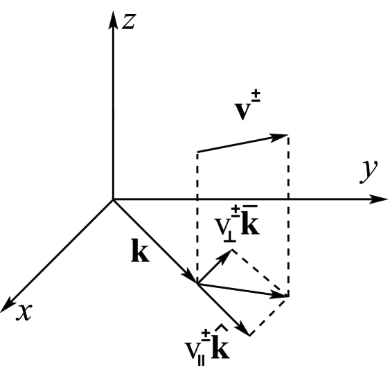
Figure 6: Projection of ${\bf v}^{\pm}[{\bf k},z]$ onto the $xy$-plane which is decomposed as $v_{\parallel}^{\pm}\hat{{\bf k}}+v_{\perp}^{\pm}\bar{{\bf k}}$.

Our derivation of the mobility tensor for the membrane closely follows that by Inaura and Fujitani inaura-08 . As presented in fig. 2, we consider a more general case where the two walls are located at different distances from the membrane, i.e., $h^{+}\neq h^{-}$. The membrane is assumed to be impermeable.

Our purpose is to derive the in-plane force ${\bf f}_{\rm s}$ on the membrane due to the bulk solvent and walls (see eq. (2)). We first take the Fourier transform of ${\bf v}^{\pm}({\bf r},z)$ by

$${\bf v}^{\pm}[{\bf k},z]=\int{\rm d}^{2}r\,{\bf v}^{\pm}({\bf r},z)\exp(-i{\bf k}\cdot{\bf r}),$$ (A.1)

where ${\bf r}=(x,y)$ and ${\bf k}=(k_{x},k_{y})$. The projection of the vector ${\bf v}^{\pm}[{\bf k},z]$ on the $xy$-plane can be expressed as $v_{\parallel}^{\pm}[{\bf k},z]\hat{{\bf k}}+v_{\perp}^{\pm}[{\bf k},z]\bar{{\bf k}}$ where $\hat{{\bf k}}=(k_{x}/k,k_{y}/k)$ and $\bar{{\bf k}}=(-k_{y}/k,k_{x}/k)$ with $k=|{\bf k}|$. The subscripts $\parallel$ and $\perp$ indicate the components parallel and perpendicular to $\hat{{\bf k}}$, respectively. From eq. (4), the vertical component $v_{\perp}^{\pm}[{\bf k},z]$ obeys the equation

$$\left(-k^{2}+\frac{\partial^{2}}{\partial z^{2}}\right)v_{\perp}^{\pm}[{\bf k},z]=0.$$ (A.2)

The solution to the above equation can be written as

$$v_{\perp}^{\pm}[{\bf k},z]=A_{1}e^{-kz}+A_{2}e^{kz},$$ (A.3)

with unknown coefficients $A_{1}$ and $A_{2}$. These coefficients are determined by the stick boundary conditions imposed at the membrane-solvent and solvent-wall boundaries:

$$v_{\perp}^{\pm}[{\bf k},z]=\begin{cases}v_{\perp}[{\bf k}]&\mbox{at}~{}~{}z=0,\\ 0&\mbox{at}~{}~{}z=\pm h^{\pm},\end{cases}$$ (A.4)

where $v_{\perp}[{\bf k}]={\bf v}[{\bf k}]\cdot\bar{{\bf k}}$ and see eq.(7) for the definition of ${\bf v}[{\bf k}]$. Thus we have

$$v_{\perp}^{\pm}[{\bf k},z]=\mp v_{\perp}[{\bf k}]\frac{\sinh(k(z\mp h^{\pm}))}{\sinh(kh^{\pm})}.$$ (A.5)

From eq. (A.5), the in-plane force on the membrane due to the outer solvent and walls becomes

$$f_{\rm s\perp}[{\bf k}] ={\bf f}_{\rm s}[{\bf k}]\cdot\bar{{\bf k}}$$

$$=\frac{\partial}{\partial z}\left(\eta^{+}_{\rm s}v_{\perp}^{+}[{\bf k},z]-\eta^{-}_{\rm s}v_{\perp}^{-}[{\bf k},z]\right)_{z=0}$$

$$=-\eta_{\rm s}^{+}v_{\perp}k\coth(kh^{+})-\eta_{\rm s}^{-}v_{\perp}k\coth(kh^{-}).$$ (A.6)

Since the incompressibility condition of the membrane fluid implies $v_{\parallel}[{\bf k}]={\bf v}[{\bf k}]\cdot\hat{{\bf k}}=0$, the perpendicular component of the Fourier transform of eq. (2) gives

$$-\eta k^{2}v_{\perp}[{\bf k}]+f_{{\rm s}\perp}[{\bf k}]+F_{\perp}[{\bf k}]=0,$$ (A.7)

with $F_{\perp}[{\bf k}]={\bf F}[{\bf k}]\cdot\bar{{\bf k}}$. Hence the mobility tensor defined by ${\bf v}[{\bf k}]={\bf G}[{\bf k}]\cdot{\bf F}[{\bf k}]$ is given by eq. (9).

Appendix B. Mobility tensors in real space

Free membrane case

The mobility tensor in Fourier space is given by eq. (11). The expression for $G^{\rm SD}_{\alpha\beta}({\bf r})$ can be found by assuming

$$G^{\rm SD}_{\alpha\beta}({\bf r})=B_{1}\delta_{\alpha\beta}+B_{2}\frac{r_{\alpha}r_{\beta}}{r^{2}},$$ (B.1)

with two coefficients $B_{1}$ and $B_{2}$. By considering the diagonal and off-diagonal parts of eq. (B.1) separately, we have

$$2B_{1}+B_{2} =\frac{1}{2\pi\eta}\int_{0}^{\infty}{\rm d}k\,\frac{J_{0}(kr)}{k+\nu}$$ (B.2)

$$=\frac{1}{4\eta}\left[{\bf H}_{0}(\nu r)-Y_{0}(\nu r)\right],$$ (B.3)

and

$$B_{1}+B_{2} =\frac{1}{2\pi\eta}\int_{0}^{\infty}{\rm d}k\,\frac{J_{1}(kr)}{kr(k+\nu)}$$ (B.4)

$$=\frac{1}{4\pi\eta}\int_{0}^{\infty}{\rm d}k\,\frac{J_{0}(kr)+J_{2}(kr)}{k+\nu}$$ (B.5)

$$=\frac{1}{4\eta}\left[-\frac{2}{\pi\nu^{2}r^{2}}+\frac{{\bf H}_{1}(\nu r)}{\nu r}-\frac{Y_{1}(\nu r)}{\nu r}\right].$$ (B.6)

See ref. gradshteyn for the integral of eq. (B.3). In evaluating the integral of eq. (B.6), we have made use of the following relations;

$$\frac{J_{1}(z)}{z}=J_{0}(z)+\frac{{\rm d}^{2}}{{\rm d}z^{2}}J_{0}(z),$$ (B.7)

$$\int_{0}^{\infty}{\rm d}z\,J_{0}(z)\frac{{\rm d}^{2}}{{\rm d}z^{2}}\frac{1}{z+a}=\frac{{\rm d}^{2}}{{\rm d}a^{2}}\int_{0}^{\infty}{\rm d}z\,\frac{J_{0}(z)}{z+a}.$$ (B.8)

Solving eqs. (B.3) and (B.6) for $B_{1}$ and $B_{2}$, we get

$$B_{1}= \frac{1}{4\eta}\left[{\bf H}_{0}(\nu r)-Y_{0}(\nu r)+\frac{2}{\pi\nu^{2}r^{2}}\right.$$

$$\left.-\frac{{\bf H}_{1}(\nu r)}{\nu r}+\frac{Y_{1}(\nu r)}{\nu r}\right],$$ (B.9)

$$B_{2}= \frac{1}{4\eta}\left[-\frac{4}{\pi\nu^{2}r^{2}}+\frac{2{\bf H}_{1}(\nu r)}{\nu r}\right.$$

$$\left.-\frac{2Y_{1}(\nu r)}{\nu r}-{\bf H}_{0}(\nu r)+Y_{0}(\nu r)\right].$$ (B.10)

The preaveraging of eq. (B.1) yields

$$g^{\rm SD}(n-m)=\frac{1}{2}\langle 2B_{1}+B_{2}\rangle.$$ (B.11)

Hence we obtain eq. (73) using eq. (B.3).

Confined membrane case

Now the mobility tensor in the Fourier space is eq. (14). Similar to the free membrane case, its real space expression can be written as

$$G^{\rm ES}_{\alpha\beta}({\bf r})=C_{1}\delta_{\alpha\beta}+C_{2}\frac{r_{\alpha}r_{\beta}}{r^{2}},$$ (B.12)

with two coefficients $C_{1}$ and $C_{2}$. Then it follows that

$$2C_{1}+C_{2} =\frac{1}{2\pi\eta}\int_{0}^{\infty}{\rm d}k\,\frac{kJ_{0}(kr)}{k^{2}+\kappa^{2}}$$ (B.13)

$$=\frac{1}{2\pi\eta}K_{0}(\kappa r),$$ (B.14)

and

$$C_{1}+C_{2} =\frac{1}{2\pi\eta}\int_{0}^{\infty}{\rm d}k\,\frac{J_{1}(kr)}{r(k^{2}+\kappa^{2})}$$ (B.15)

$$=\frac{1}{2\pi\eta}\left[\frac{1}{\kappa^{2}r^{2}}-\frac{K_{1}(\kappa r)}{\kappa r}\right].$$ (B.16)

Solving these equations, we obtain

$$C_{1} =\frac{1}{2\pi\eta}\left[K_{0}(\kappa r)+\frac{K_{1}(\kappa r)}{\kappa r}-\frac{1}{\kappa^{2}r^{2}}\right],$$ (B.17)

$$C_{2} =\frac{1}{2\pi\eta}\left[-K_{0}(\kappa r)-\frac{2K_{1}(\kappa r)}{\kappa r}+\frac{2}{\kappa^{2}r^{2}}\right].$$ (B.18)

References

- (1) B. Alberts, A. Johnson, P. Walter, J. Lewis, M. Raff, Molecular Biology of the Cell (Garland Science, New York, 2008)
- (2) R. Peters, R.J. Cherry, Proc. Natl. Acad. Sci. USA 79, 4317 (1982)
- (3) E.A.J. Reitz, J.J. Neefjes, Nat. Cell Biol. 3, E145 (2001)
- (4) N. Kahya, E.-I. Pécheur, W.P. de Boeij, D.A. Wiersam, D. Hoekstra, Biophys. J. 81, 1464 (2001)
- (5) N. Tsapis, F. Reiss-Husson, R. Ober, M. Genest, R.S. Hodges, W. Urbach, Biophys. J. 81, 1613 (2001)
- (6) Y. Gambin, R. Lopez-Esparza, M. Reffay, E. Sierecki, N.S. Gov, M. Genest, R.S. Hodges, W. Urbach, Proc. Natl. Acad. Sci. USA 103, 2098 (2007)
- (7) D.F. Kucik, E.L. Olson, M.P. Sheetz, Biophys. J. 76, 314 (1999)
- (8) J. Lippincott-Schwartz, E. Snapp, A. Kenworthy, Nat. Rev. Mol. Cell Biol. 2, 444 (2001)
- (9) M. Vrljic, Y. Nishimura, S. Brasselet, W.E. Moerner, H.M. McConnell, Biophys. J. 83, 2681 (2002)
- (10) A.K. Kenworthy, B.J. Nichols, C.L. Remmert, G.M. Hendrix, M. Kumar, J. Zimmerberg, J. Lippincott-Schwartz, J. Cell. Biol. 165, 735 (2004)
- (11) P.G. Saffman, M. Delbrück, Proc. Natl. Acad. Sci. USA 72, 3111 (1975)
- (12) P.G. Saffman, J. Fluid Mech. 73, 593 (1976)
- (13) B.D. Hughes, B.A. Pailthorpe, L.R. White, J. Fluid Mech. 110, 349 (1981)
- (14) E. Evans, E. Sackmann, J. Fluid Mech. 194, 553 (1988)
- (15) Y. Tserkovnyak, D.R. Nelson, Proc. Natl. Acad. Sci. USA 103, 15002 (2006)
- (16) A.J. Levine, T.B. Liverpool, F.C. MacKintosh, Phys. Rev. Lett. 93, 038102 (2004)
- (17) A.J. Levine, T.B. Liverpool, F.C. MacKintosh, Phys. Rev. E 69, 021503 (2004)
- (18) Th.M. Fischer, J. Fluid Mech. 498, 123 (2004)
- (19) Y. Yang, R. Prudhomme, K.M. McGrath, P. Richetti, C.M. Marques, Phys. Rev. Lett. 12, 2729 (1998)
- (20) M. Muthukumar, J. Chem. Phys. 82, 5696 (1985)
- (21) S. Komura, K. Seki, J. Phys. II 5, 5 (1995)
- (22) S. Ramaswamy, G.F. Mazenko, Phys. Rev. A 26, 1735 (1982)
- (23) Y.Y. Suzuki, T. Izuyama, J. Phys. Soc. Japan 58, 1104 (1989)
- (24) K. Seki, S. Komura, Phys. Rev. E 47, 2377 (1993)
- (25) K. Seki, S. Komura, M. Imai, J. Phys.: Condens. Matter 19, 072101 (2007)
- (26) B. Maier, J.O. Rädler, Phys. Rev. Lett. 82, 1911 (1999)
- (27) B. Maier, J.O. Rädler, Macromolecules 33, 7185 (2000)
- (28) B. Maier, J.O. Rädler, Macromolecules 34, 5723 (2001)
- (29) C. Herold, P. Schwille, E.P. Petrov, Phys. Rev. Lett. 104, 148102 (2010)
- (30) M. Daoud, P.G. de Gennes, J. Phys. 38, 85 (1977)
- (31) F. Brochard, J. Phys. 38, 1285 (1977)
- (32) P.G. de Gennes, F. Brochard, J. Chem. Phys. 67, 52 (1977)
- (33) T. Tlusty, Macromolecules 39, 3927 (2006)
- (34) P.K. Lin, C.C. Fu, Y.R. Chen, P.K. Wei, C.H. Kuan, W.S. Fann, Phys. Rev. E 76, 011806 (2007)
- (35) K. Inaura, Y. Fujitani, J. Phys. Soc. Jpn. 77, 114603 (2008)
- (36) M. Kraus, U. Seifert, J. Phys. II 4, 1117 (1994)
- (37) N. Gov, A.G. Zilman, S. Safran, Phys. Rev. E 70, 011104 (2004)
- (38) S. Sankararaman, G.I. Menon, P.B.S. Kumar, Phys. Rev. E 66, 031914 (2002)
- (39) D.K. Lubensky, R.E. Goldstein, Phys. Fluids 8, 843 (1996)
- (40) N. Oppenheimer, H. Diamant, Biophys. J. 96, 3041 (2009)
- (41) N. Oppenheimer, H. Diamant, Phys. Rev. E 82, 041912 (2010)
- (42) H. Stone, A. Ajdari, J. Fluid Mech. 369, 151 (1998)
- (43) S. Ramachandran, S. Komura, M. Imai, K. Seki, Eur. Phys. J. E 31, 303 (2010)
- (44) D.L. Ermak, J.A. McCammon, J. Chem. Phys. 69, 1352 (1978)
- (45) M. Doi, S.F. Edwards, The Theory of Polymer Dynamics (Clarendon Press, Oxford, 1986)
- (46) B.H. Zimm, J. Chem. Phys. 24, 269 (1956)
- (47) W. Feller, An Introduction to Probability Theory and its Applications (Wiley, New York, 1968)
- (48) M. Abramowitz, I.A. Stegun, Handbook of Mathematical Functions (Dover, New York, 1972)
- (49) S. Ramachandran, S. Komura, G. Gompper, Europhys. Lett. 89, 56001 (2010)
- (50) H. Diamant, J. Phys. Soc. Jpn. 78, 041002 (2009)
- (51) M. Rubinstein, R.H. Colby, Polymer Physics (University Press, Oxford, 2004)
- (52) R.M. Johnson, J.L. Schrag, J.D. Ferry, Polymer J. 1, 742 (1970)
- (53) W.H. Stockmayer, B. Hammouda, Pure Appl. Chem. 56, 1373 (1984)
- (54) Y. Kaizuka, J.T. Groves, Biophys. J. 86, 905 (2004)
- (55) I.S. Gradshteyn, I.M. Ryzhik, Table of Integrals, Series and Products (Academic Press, London, 1994)