Study of fragmentation and momentum correlations in heavy-ion collisions
Sakshi Gautam and Rajni Kant
Department of Physics, Panjab University, Chandigarh -160 014, India.

The role of momentum correlations is studied in the production of light and medium mass fragments by imposing momentum cut in clusterization the phase space. Our detailed investigation shows that momentum cut has major role to play in the emission of fragments.

1 Introduction

It is well known that colliding nuclei break into several small and medium size pieces and a lot of nucleons are also emitted. This subfield, known as multifragmentation, gained momentum after several theoretical and experimental groups around the world put their collective efforts to understand this process [1]. Because of accumulation of experimental data on multifragmentation, one has the opportunity to study the role of dynamical correlations in fragment formation. Theoretically, the availability of large number of models makes the situation worse [1, 2, 3, 4]. Due to fact that fragmentation need fluctuations and correlations, the molecular dynamical models are the only resource in theoretical domains. The molecular dynamics (n-body) approach is well suited as it incorporates the correlations and fluctuations among the nucleons. We will, therefore, use quantum molecular dynamics (QMD) model [2, 3] to study the dynamics of heavy-ion collisions. Since every model simulate single nucleon, one needs to have afterburner to clusterize the phase space. In a very simple picture, we can define a cluster by using space correlations. This method is known as minimum spanning tree (MST) method [5]. In this method, we allow nucleons to form a cluster if their centroids are less than 4 fm. This method works fine when the system is very dilute. At the same time fragments formed in MST method will be highly unstable (especially in central collisions) as there the two nucleons may not be well formed and therefore can be unstable that will decay after a while. In order to filter out such unstable fragments, we impose another cut in terms of relative momentum of nucleons. This method, dubbed as minimum spanning tree with momentum cut (MSTP) method was discussed by Puri et al. [6]. Unfortunately this study was restricted to heavier systems like ⁹³Nb+⁹³Nb and ¹⁹⁷Au+¹⁹⁷Au reactions. The role of momentum cut on the fragment structure of lighter systems is still unclear. We aim to address this in present paper.

Exclusively we plan to
(i) see the role of momentum cut on the fragment structure of lighter colliding systems.
(ii) and see the role of colliding geometry on the fragment structure with momentum cut being imposed.
The present study is carried out within the framework of QMD model [2, 3] which is described in the following section.

2 The Formalism

2.1 Quantum Molecular dynamics (QMD) model

We describe the time evolution of a heavy-ion reaction within the framework of Quantum Molecular Dynamics (QMD) model [2, 3] which is based on a molecular dynamics picture. This model has been successful in explaining collective flow [7], elliptic flow [8], multifragmentation [9] as well as dense and hot matter [10]. Here each nucleon is represented by a coherent state of the form

$$\phi_{\alpha}(x_{1},t)=\left({\frac{2}{L\pi}}\right)^{\frac{3}{4}}e^{-(x_{1}-x_{\alpha}(t))^{2}}e^{ip_{\alpha}(x_{1}-x_{\alpha})}e^{-\frac{ip_{\alpha}^{2}t}{2m}}.$$ (1)

Thus, the wave function has two time dependent parameters $x_{\alpha}$ and $p_{\alpha}$. The total n-body wave function is assumed to be a direct product of coherent states:

$$\phi=\phi_{\alpha}(x_{1},x_{\alpha},p_{\alpha},t)\phi_{\beta}(x_{2},x_{\beta},p_{\beta},t)....,$$ (2)

where antisymmetrization is neglected. One should, however, keep in the mind that the Pauli principle, which is very important at low incident energies, has been taken into account. The initial values of the parameters are chosen in a way that the ensemble ($A_{T}$+$A_{P}$) nucleons give a proper density distribution as well as a proper momentum distribution of the projectile and target nuclei. The time evolution of the system is calculated using the generalized variational principle. We start out from the action

$$S=\int_{t_{1}}^{t_{2}}{\cal{L}}[\phi,\phi^{*}]d\tau,$$ (3)

with the Lagrange functional

$${\cal{L}}=\left(\phi\left|i\hbar\frac{d}{dt}-H\right|\phi\right),$$ (4)

where the total time derivative includes the derivatives with respect to the parameters. The time evolution is obtained by the requirement that the action is stationary under the allowed variation of the wave function

$$\delta S=\delta\int_{t_{1}}^{t_{2}}{\cal{L}}[\phi,\phi^{*}]dt=0.$$ (5)

If the true solution of the Schrödinger equation is contained in the restricted set of wave function $\phi_{\alpha}\left({x_{1},x_{\alpha},p_{\alpha}}\right),$ this variation of the action gives the exact solution of the Schrödinger equation. If the parameter space is too restricted, we obtain that wave function in the restricted parameter space which comes close to the solution of the Schrödinger equation. Performing the variation with the test wave function (2), we obtain for each parameter $\lambda$ an Euler-Lagrange equation;

$$\frac{d}{dt}\frac{\partial{\cal{L}}}{\partial{\dot{\lambda}}}-\frac{\partial\cal{L}}{\partial\lambda}=0.$$ (6)

For each coherent state and a Hamiltonian of the form,

$H=\sum_{\alpha}\left[T_{\alpha}+{\frac{1}{2}}\sum_{\alpha\beta}V_{\alpha\beta}\right]$, the Lagrangian and the Euler-Lagrange function can be easily calculated [aich2]

$${\cal{L}}=\sum_{\alpha}{\dot{\bf x}_{\alpha}}{\bf p}_{\alpha}-\sum_{\beta}\langle{V_{\alpha\beta}}\rangle-\frac{3}{2Lm},$$ (7)

$${\dot{\bf x}_{\alpha}}=\frac{{\bf p}_{\alpha}}{m}+\nabla_{p_{\alpha}}\sum_{\beta}\langle{V_{\alpha\beta}}\rangle,$$ (8)

$${\dot{\bf p}_{\alpha}}=-\nabla_{{\bf x}_{\alpha}}\sum_{\beta}\langle{V_{\alpha\beta}}\rangle.$$ (9)

Thus, the variational approach has reduced the n-body Schrödinger equation to a set of 6n-different equations for the parameters which can be solved numerically. If one inspects the formalism carefully, one finds that the interaction potential which is actually the Brückner G-matrix can be divided into two parts: (i) a real part and (ii) an imaginary part. The real part of the potential acts like a potential whereas imaginary part is proportional to the cross section.

In the present model, interaction potential comprises of the following terms:

$$V_{\alpha\beta}=V_{loc}^{2}+V_{loc}^{3}+V_{Coul}+V_{Yuk}$$ (10)

$V_{loc}$ is the Skyrme force whereas $V_{Coul}$, $V_{Yuk}$ and $V_{MDI}$ define, respectively, the Coulomb, and Yukawa potentials. The Yukawa term separates the surface which also plays the role in low energy processes like fusion and cluster radioactivity [12]. The expectation value of these potentials is calculated as

$$V^{2}_{loc} = \int f_{\alpha}({\bf p}_{\alpha},{\bf r}_{\alpha},t)f_{\beta}({\bf p}_{\beta},{\bf r}_{\beta},t)V_{I}^{(2)}({\bf r}_{\alpha},{\bf r}_{\beta})$$ (11)

$$\times{d^{3}{\bf r}_{\alpha}d^{3}{\bf r}_{\beta}d^{3}{\bf p}_{\alpha}d^{3}{\bf p}_{\beta},}$$

$$V^{3}_{loc} = \int f_{\alpha}({\bf p}_{\alpha},{\bf r}_{\alpha},t)f_{\beta}({\bf p}_{\beta},{\bf r}_{\beta},t)f_{\gamma}({\bf p}_{\gamma},{\bf r}_{\gamma},t)$$ (12)

$$\times V_{I}^{(3)}({\bf r}_{\alpha},{\bf r}_{\beta},{\bf r}_{\gamma})d^{3}{\bf r}_{\alpha}d^{3}{\bf r}_{\beta}d^{3}{\bf r}_{\gamma}$$

$$\times d^{3}{\bf p}_{\alpha}d^{3}{\bf p}_{\beta}d^{3}{\bf p}_{\gamma}.$$

where $f_{\alpha}({\bf p}_{\alpha},{\bf r}_{\alpha},t)$ is the Wigner density which corresponds to the wave functions (eq. 2). If we deal with the local Skyrme force only, we get

$$V^{Skyrme}=\sum_{{\alpha}=1}^{A_{T}+A_{P}}\left[\frac{A}{2}\sum_{{\beta}=1}\left(\frac{\tilde{\rho}_{\alpha\beta}}{\rho_{0}}\right)+\frac{B}{C+1}\sum_{{\beta}\neq{\alpha}}\left(\frac{\tilde{\rho}_{\alpha\beta}}{\rho_{0}}\right)^{C}\right].$$ (13)

Here A, B and C are the Skyrme parameters which are defined according to the ground state properties of a nucleus. Different values of C lead to different equations of state. A larger value of C (= 380 MeV) is often dubbed as stiff equation of state.The finite range Yukawa ($V_{Yuk}$) and effective Coulomb potential ($V_{Coul}$) read as:

$$V_{Yuk}=\sum_{j,i\neq j}t_{3}\frac{exp\{-|\textbf{r}_{\textbf{i}}-\textbf{r}_{\textbf{j}}|\}/\mu}{|\textbf{r}_{\textbf{i}}-\textbf{r}_{\textbf{j}}|/\mu},$$ (14)

$$V_{Coul}=\sum_{j,i\neq j}\frac{Z_{eff}^{2}e^{2}}{|\textbf{r}_{\textbf{i}}-\textbf{r}_{\textbf{j}}|}.$$ (15)

The Yukawa interaction (with $t_{3}$= -6.66 MeV and $\mu$ = 1.5 fm) is essential for the surface effects. The relativistic effect does not play role in low incident energy of present interest [11].

The phase space of nucleons is stored at several time steps. The QMD model does not give any information about the fragments observed at the final stage of the reaction. In order to construct the fragments, one needs clusterization algorithms. We shall concentrate here on the MST and MSTP methods.

According to MST method [5], two nucleons are allowed to share the same fragment if their centroids are closer than a distance $r_{min}$,

$$|\textbf{r}_{\textbf{i}}-\textbf{r}_{\textbf{j}}|\leq r_{min}.$$ (16)

where $\textbf{r}_{\textbf{i}}$ and $\textbf{r}_{\textbf{j}}$ are the spatial positions of both nucleons and r_min taken to be 4fm.

For MSTP method,we impose a additional cut in the momentum space, i.e., we allow only those nucleons to form a fragment which in addition to equation(16) also satisfy

$$|\textbf{p}_{\textbf{i}}-\textbf{p}_{\textbf{j}}|\leq p_{min},$$ (17)

where p_min = 150 MeV/c.

3 Results and Discussion

We simulated the reactions of ¹²C+¹²C , ⁴⁰Ca+⁴⁰Ca, ⁹⁶Zr+⁹⁶Zr and ¹⁹⁷Au+¹⁹⁷Au at 100 and 400 MeV/nucleon at $\hat{b}$ = 0.0, 0.2, 0.4, 0.6 and 0.8. We use a soft equation of state with standard energy-dependent Cugon cross section.

Figure 1: The time evolution of A^max, free nucleons and LCPs for the reaction of ¹²C+¹²C at incident energy of 100 (left panels) and 400 MeV/nucleon (right) with MST and MSTP methods, respectively.

Figure 2: Same as Fig. 1 but for the reaction of ⁴⁰Ca+⁴⁰Ca.

In Figure 1, we display the time evolution of A^max[(a),(b)], free nucleons [(c),(d)] and LCPs(2$\leq$A$\leq$4) [(e),(f)] for the reactions of ¹²C+¹²C at 100 (left panels) and 400 (right) MeV/nucleon. Solid lines indicate the results of MST method whereas dashed lines represent the results of MSTP method. The heaviest fragment A^max follows different time evolution in MSTP as compared to MST method. In MST, we have a single big fragment whereas momentum cut gives two distinct fragments which shows realistic picture.

In Figure 1(c) and 1(d), we display the time evolution of free nucleons. We see that for both the energies, MSTP method yields more free nucleons compared to MST method. There is also a delayed emission of nucleons in MST because of no restrictions being imposed. This delayed emission of free nucleons in MST method taken place because of the fact that till 30 fm/c, we have a single big fragment in MST method (See Figure 1(a),(b)). The fragments saturate earlier in MSTP than MST as predicted in Ref. [6].

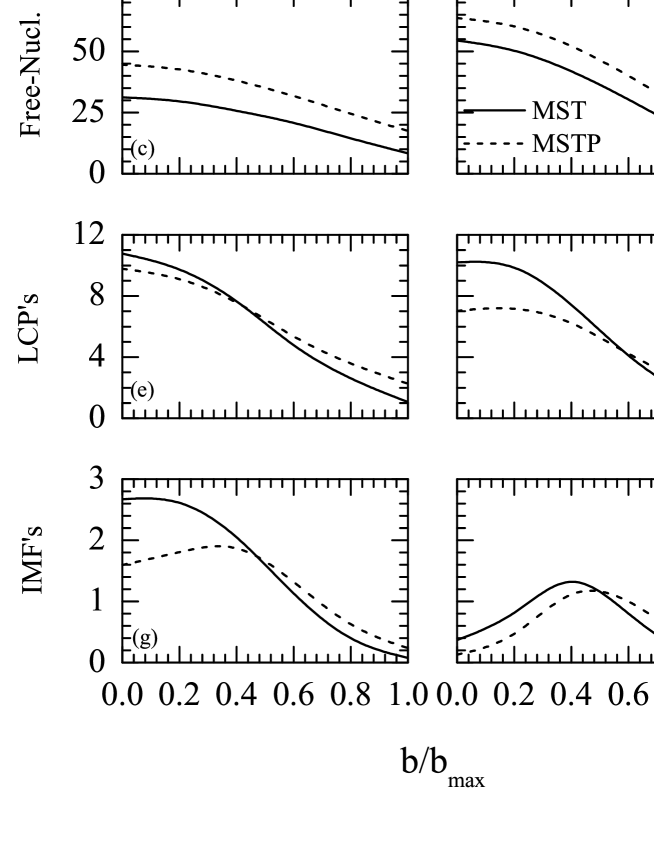
Figure 3: The impact parameter dependence of A^max, free nucleons, LCPs and IMFs for the reaction of ⁴⁰Ca+⁴⁰Ca at 100 (left panels) and 400 (right) MeV/nucleon with MST and MSTP methods.

In figure 1 [(e),(f)], we display the time evolution of LCPs. We see that MST yields more LCPs. The difference between MST and MSTP method increases at 400 Mev/nucleon signifying significant role of momentum correlations at higher incident energies.

Figure 4: Same as Fig. 3 but for the reaction of ⁹⁶Zr+⁹⁶Zr.

Figure 5: Same as Fig. 3 but for the reaction of ¹²C+¹²C.

In figure 2, we display the time evolution of A^max, free nucleons, LCPs and IMFs for the reactions of ⁴⁰Ca+⁴⁰Ca respectively at 100 (left panel) and 400 (right) MeV/nucleon. We see that A^max and free nucleons follow similar behavior as reported for the reactions of ¹²C+¹²C. The emission of free nucleons enhances with the cut and thus reducing the number of LCPs and IMFs. Similar effects also seen for the reaction of ⁹⁶Zr+⁹⁶Zr.

In figures 3 and 4, we display the impact parameter dependence of A^max, free nucleons, LCPs, and IMFs for the reaction of ⁴⁰Ca+⁴⁰Ca and ⁹⁶Zr+⁹⁶Zr, respectively, at 100(left panel) and 400 (right) MeV/nucleon. From both figures we see that A^max rises with impact parameter for both methods uniformly. The difference increases with impact parameter. This happens because of the fact that we have a bigger spectator matter (from where A^max generates) at peripheral collisions geometry. The number of free nucleons decreases with increase in impact parameter for both methods.

Figure 6: The system size dependence of the percentage difference of A^max and free nucleons between MST and MSTP at various impact parameters. Lines represent the average values.

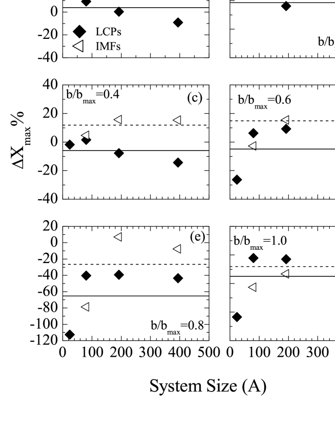
Figure 7: Same as Fig. 6, but for the LCPs and IMFs.

The emission of fragments shows that in contrast to central collisions, peripheral collisions does not show drastic changes with method. This happens due to fact that with increase in colliding geometry, the fragments are the reminants of either projectile or target, therefore breaking mechanisms are almost bound and therefore MSTP methods does not give different results.

In figure 5, we display the impact parameter dependence of A^max, free nucleons, and LCPs for the reaction of ¹²C+¹²C at 100 (left panel) and 400 (right) MeV/nucleon. We see that in this particular case, the effect of momentum cut on the fragment production enhances with impact parameter (see figure 6(e) and (f)) which is quite different compared to earlier figures. This is because the spectator matter even at peripheral geometries will be very less in such a lighter system and so the fragments are emitted mostly from the participant region, where they are unstable and hence momentum cut plays a role at such geometries.

In figure 6, we display the percentage difference [$(\Delta X($%$)=(X_{(mst)}-X_{(mstp)}/X_{mst})\times 100)$]. We display the system size dependence of the percentage difference of the quantities A^max and free nucleons at $\hat{b}$= 0.0, 0.2, 0.4, 0.6 and 0.8. We see that percentage difference of A^max (circles) is almost constant and remains independent of system size at central and semicentral colliding geometry where it is more for lighter systems at peripheral colliding geometries. Similar behavior is also observed for the free nucleons.

In figure 7, we display the system size dependence of the percentage difference of LCPs and IMFs at various impact parameters. From figure we see that in central collision, $\Delta$IMF% is almost independent of the system size whereas at peripheral colliding geometries it increases with system mass. The average difference is 22, 69, -45, and -16 for A^max, free nucleons, LCPs, and IMFs, respectively.

4 Summary

Using quantum molecular dynamic model,we studied the role of momentum correlations in fragmentation. This was achieved by imposing cut in momentum space during the process of clusterization. We find that this cut yields significant difference in the multifragmentations of system at all colliding geometries.

5 Acknowledgement

This work is done under the supervision of Dr. Rajeev K. Puri, Department of Physics, Panjab University, Chandigarh, India. This work has been supported by a grant from Centre of Scientific and Industrial Research (CSIR), Govt. of India.

References

- [1] M. Begemann-Blaich, Phys. Rev. C 48, 610 (1993); M. B. Tsang et al., Phys. Rev. Lett. 71, 1502 (1993); D. R. Bowmann et al., Phys. Rev. Lett. 67, 1527 (1991); W. Reisdorf et al., Nucl. Phys. A612, 493 (1997); W. Bauer, G. F. Bertsch and H. Schulz, Phys. Rev. Lett. 69, 1888 (1992).
- [2] J. Aichelin, Phys. Rep. 202, 233 (1991).
- [3] J. Singh, S. Kumar, and R. K. Puri, Phys. Rev. C 62, 044617 (2000); R. K. Puri and J. Aichelin, J. Comput. Phys. 162, 245 (2000); Y. K. Vermani, J. K. Dhawan, S. Goyal, R. K. Puri, and J. Aichelin, J. Phys. G: Nucl. Part. Phys. 37, 015105 (2010); ibid. G 36, 105103 (2009); Y. K. Vermani and R. K. Puri, Europhys. Lett. 85, 62001 (2009); A. D. Sood and R. K. Puri, Phys. Rev. C 79, 064618 (2009); ibid. C 79, 064613 (2009).
- [4] C. Dorso and J. Randrup, Phys. Lett. B301, 328 (1993).
- [5] J. Singh and R. K. Puri, J. Phys. G: Nucl. Part. Phys. 27, 2091 (2001); ibid. Phys. Rev. C 62, 054602 (2000).
- [6] S. Kumar and R. K. Puri, Phys. Rev. C 78, 064602 (2008); ibid. C 58, 320 (1998); ibid. C 57, 2744 (1998).
- [7] A. D. Sood et al., Phys. Lett. B 594, 260 (2004); ibid., Phys. Rev. C 70, 034611 (2004); ibid. C 69, 054612 (2004); ibid. C 73, 067602 (2006); ibid., Eur. Phys. J A 30, 571 (2006); R. Chugh et al., Phys. Rev. C 82, 014603 (2010); S. Goyal et al., Nucl. Phys. A 853, 164 (2011); S. Gautam et al., J. Phys. G: Nucl. Part. Phys. 37, 085102 (2010); ibid., Phys. Rev. C 83, 014603 (2011).
- [8] S. Kumar et al., Phys. Rev. C 81, 014601 (2010); ibid. C 81, 014611 (2010); V. Kaur et al., Phys. Lett. B 697, 512 (2011).
- [9] J. Dhawan et al., Phys. Rev. C 74, 057901 (2006); ibid. C 74, 057610 (2006).
- [10] C. Fuchs et al., J. Phys. G: Nucl. Part. Phys. 22, 131 (1996); Y. K. Vermani et al., Nucl. Phys. A 847, 243 (2010); G. Batko et al., J. Phys. G: Nucl. Part. Phys. 20, 461 (1994); S. W. Huang et al., Prog. Part. Phys. 30, 105 (2003).
- [11] E. Lehmann et al., Phys. Rev. C 51, 2113 (1995); ibid., Prog. Part. Nucl. Phys. 30, 219 (1993).
- [12] R. K. Puri et al., J. Phys. G: Nucl. Part. Phys. G 18, 903 (1992); ibid., G18, 1533 (1992); ibid., Phys. Rev. C 45, 1837 (1992); ibid., C 43, 315 (1991); ibid., Eur. Phys. J. A 3, 277 (1998); ibid. A23, 429 (2005); ibid., Eur. Phys. J. A 8, 103 (2008); S. S. Malik et al., Pramana J. Phys. 32, 419 (1989); I. Dutt et al., Phys. Rev. C 81, 064608 (2010); ibid. C 81, 064609 (2010); ibid. C 81, 047601 (2010); ibid. C 81, 044615 (2010).