Lattice SU(3) thermodynamics and the onset of perturbative behaviour
Abstract:
We present the equation of state (pressure, trace anomaly, energy density and entropy density) of the SU(3) gauge theory from lattice field theory in an unprecedented precision and temperature range. We control both finite size and cut-off effects. The studied temperature window () stretches from the glueball dominated system into the perturbative regime, which allows us to discuss the range of validity of these approaches. From the critical couplings on fine lattices we get and use this ratio to express the perturbative free energy in units. We also determine the preferred renormalization scale of the Hard Thermal Loop scheme and we fit the unknown order perturbative coefficient at extreme high temperatures . We furthermore quantify the nonperturbative contribution to the trace anomaly using two simple functional forms.
1 Introduction
The general feature of asymptotic freedom makes weak coupling approaches very natural in non-abelian gauge theories, such as the SU(3) model, which describes the gluonic degrees of freedom of Quantum Chromodynamics. At asymptotically high temperatures low orders of perturbation theory may be acceptable, but at any lower scale that could be probed by a realistic experiment an extension is necessary: either by the inclusion of very high order diagrams, or by an efficient resummation scheme, such as Hard Thermal Loops (HTL). Note however that analytic perturbative expansions are plagued by infrared divergences due to which the series can be computed only up to a given finite order. There is strong simulation evidence that at low temperatures ( MeV) the gluonic matter freezes and a first order transition takes place. At even lower temperatures colorless non-perturbative excitations govern the thermodynamics. To describe the phase transition or the glueball gas no weak coupling scheme succeeds and one has to rely on a natively non-perturbative approach, such as lattice field theory.
The past year witnessed considerable achievements on the side of the analytical results. The HTL scheme has been used to calculate the pure SU(3) gauge theory’s thermodynamic potential to the next-to-next-to-leading order (NNLO) [1]. The authors used their results at intermediate temperatures () where existing lattice data were available. Later the same authors have extended their results to full QCD (with massless quarks) [2] and found good agreement with the lattice data of the Wuppertal-Budapest collaboration [3] from about 300 MeV.
In conventional perturbation theory even higher orders can be computed by dimensional reduction. The full expression up to order is given in [4] and was compared to the Bielefeld lattice data [5] at . Fitting the pressure (thermodynamic potential) the slope of the pressure curve was succesfully predicted. This raised hope that at this high order perturbation theory does possess some predictive power at phenomenological temperatures. In this work we repeat this fitting procedure at a much higher temperature, where the sixth order can be shown to be a minor correction to the fifth order. Instead of treating the soft sector strictly perturbatively a screened perturbation theroy can be formulated for the dimensionally reduced theory, resulting in significantly better convergence of the free energy [6].
For more than a decade the renowned paper by Boyd et al [5] has been the reference lattice simulation of the SU(3) theory in the temperature range of . It uses the plaquette gauge action at up to lattice spacing and an aspect ratio of 4. Here denotes the number of lattice points in the Euclidean time direction, meaning that the lattice spacing at any given temperature is . The fixed approach has been introduced in Ref. [7] and this work follows it, too. It implies that the lattice spacing varies with temperature. Continuum limit is achieved by performing an extrapolation on the data at a set of fixed physical temperatures. The aspect ratio sets the ratio between space and time-like lattice points.
Since the publication of [5] several similar simulations were performed to study pure gauge theory. The equation of state has been recalculated using the Symanzik improved gauge action [8]. This set of simulations have been further generalized to SU() theories with in Refs. [9, 10]. Alternatively, the equation of state can also be calculated by fixing the lattice spacing, and using for tuning the temperature [11]. This approach is mostly advantageous with Wilson-type dynamical fermions, and less economic for the pure gluonic theory.
In most fixed simulation projects, like Ref. [5], the aspect ratio is kept constant to allow the use of a single lattice geometry. This means that higher temperatures are simulated at smaller volumes. Length scales that are present in (resummed) perturbative calculations, such as , and are normally well accommodated in the lattice, since the renormalized coupling drops only logarithmically as the temperature increases. Yet, to establish the range of validity of the perturbative approach itself, one has to simulate the non-perturbative scale, too. In this sense, the aspect ratio sets the maximum temperature as a precondition for the non-perturbativeness of the simulation: . In most previous works this was set to .
2 Simulation setup
In this work we calculate the continuum equation of state of the SU(3) theory using tree-level Symanzik improvement in the temperature range of (on , and lattices). We also support this continuum extrapolation using an additional set of lattices () below . Furthermore we present a non-continuum data set that is valid up to approximately (on a lattice) and study finite volume effects using various smaller boxes. Finally, from our third set of simulations we calculate the continuum equation of state in a small box (on , and lattices) up to 1000 . These latter data we use to find the optimal free parameters of existing perturbative calculations, e.g. the preferred renormalization scale for the HTL scheme. The precision of our data points exceeds any previous calculation by about an order of magnitude.
Although the lattice techniques for the analysis as well as for the generation of lattice configurations have been well established, achieving the presented statistics was a very challenging procedure. As explained in Ref. [7], the normalized trace anomaly is determined first. The normalized pressure and energy density are calculated using thermodynamic relations. The trace anomaly contains a quartic divergence, which is subtracted using lattice measurements of the same quantity (at the same lattice spacing) at a smaller temperature. Because of this divergence the trace anomaly is rather difficult to measure. Moreover, the value of reduces rapidly with temperature as one moves away from the transition region in either direction.
Another challenging issue was the accurate determination of the non-perturbative beta function corresponding to the Symanzik improved action. Instead of using the string tension or the Sommer parameter, it was advantageous to define the lattice spacing in terms of the transition temperature. To this end we determined the critical couplings up to from the peak of the Polyakov loop susceptibility. Matching to the universal two-loop running (in terms of the improved coupling in the “E” scheme [12], generalized for the case of the Symanzik improved action) we determined the lambda parameter in terms of the transition temperature: . (The error is overwhelmingly systematic and reflects the sensitivity to various continuum extrapolations.) This is consistent with the combination of previous determinations: the Lambda parameter of [13] can be translated to units using (based on [14]) and then used with of Ref. [5]. Through our direct result for one can easily translate the scale setting of the perturbative expression for the SU(3) free energy to the lattice language.
Given the beta function one can simply relate the expectation value of the gauge action (a weighted sum of and plaquettes) to [7]. In the standard lattice renormalization scheme this result is then subtracted from the value corresponding to zero temperature. This would require a lattice with a large temporal size. In order to be able to fit larger lattices into the given memory of our computer system we used half-temperature subtraction, i.e. we calculated along the lines of our previous work [15]. To finally arrive at this partial result was supplemented with another set of simulations at half temperature, double lattice spacing, but same physical volume. For these supplementary data we used the standard renormalization subtracting the vacuum. The continuum limit from this combined technique is equal to what one finds using the stardard scheme.
3 Results
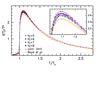
We start the presentation of the results with the reproduction of the Boyd et. al. data [5] in the left side of figure 1. We fit our four large-volume data sets with different lattice spacings altogether, using an -dependent spline function. As a result we have a smooth function interpolating our data for each (colored lines in the figure), together with a smooth, continuum extrapolated curve (yellow band in the figure). The systematic error coming from this extrapolation procedure and the statistical error are added in quadrature. We see a small discrepancy between our results and Ref. [5], which might be attributed to the scale setting assuptions in [5].
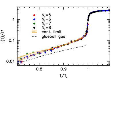
Zooming in to the low temperure region we can explore the thermodynamics of the confined phase. To find out to what extent glueballs dominate, we calculated the trace anomaly contribution of the first twelve glueballs in Ref. [16] and plotted this together with our lattice results in the right side of figure. 1. It has been suggested in Ref. [17] that the apparent deficit between the lattice data might be explained if we allow a temperature dependence for the glueballs. This dependence has already been determined for the 0++ and 2++ states [18]. This point was raised when only a couple of inprecise simulation points existed below from Panero’s data set [9]. Our data is in fairly good agreement with this scenario, however, further studies are needed to understand the question in more detail.
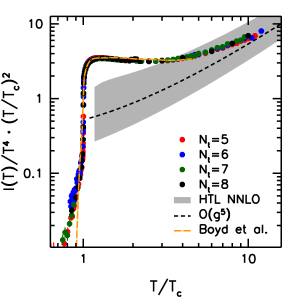
The strong non-perturbative effects in the equation of state can be emphasized by plotting instead of normalizing it to (left side of figure 2). For dimensional reasons, any finite order perturbative formula will only contribute logarithmic corrections to the Stefan-Boltzmann law. Now plotting we expect to see a curve times logarithmic corrections. What lattice data, actually, does show, is an approximately linear section up to temperature, which then connects to the perturbative estimate. This linear segment was more striking in the Bielefeld lattice data [5], since the somewhat bigger errors hid a more complex structure. Moreover the latter data set ended at a temperature where the non-perturbative behaviour was still dominant. The observed non-perturbative pattern induced speculations on a “fuzzy” bag model [19] and potential explanations in terms of a dimension-2 gluon condensate emerged [20, 21].
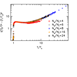
In this work we do not go into the viability of various explanations to the apparent behaviour of , but we identify it as the dominant non-perturbative effect in the deconfined phase. Its effect reduces at high temperatures and becomes unnoticeable from the lattice equation of state, independently whether or not the lattice volume accommodates the inverse scale. One way of discussing the relevance of the scale in the dynamics is to compare the trace anomaly at various volumes, as we do in the right side of figure 2 for one lattice resolution. The “standard” aspect ratio gives somewhat smaller values, but beyond our simulation is not capable of resolving the difference.
We summarize our findings as i) the large volume lattice trace anomaly data shows qualitative (and as we find using the fitted order coefficient, also quantitative, see later) agreement with the perturbative results from , and ii) we see no deviation between results from various volumes (with ), moreover iii) the dominant non-perturbative contribution loses significance as . These considerations suggest that – even if the lattice volumes are ever shrinking as the temperature is increased – our results are able to describe the physical trace anomaly (and its integral, the thermodynamic potential) within the error bars shown. Of course, this assumes that all perturbatively relevant scales are properly accounted for.
Even in the small-volume simulations presented in this paper the lattices do accommodate the ultrasoft scale . This encourages us to use these very high temperature lattice data to extract some information on the ultrasoft physics. At high enough temperatures, where the order is known to give a small correction to the order one can fit the coefficient for the perturbative result, and the preferred renomalization scale for the HTL result. For the latter we find that our lattice data prefers , with the numbers in the parentheses from left to right representing the statistical error, the error coming from the lattice scale and that from the variation of the fit interval. Repeating the fit in Ref. [4] we get for the sixth order coefficient , in the same notation for the errors. We used these data in the left and right side of Fig˙3 to compare our small volume simulations with the theoretical results.
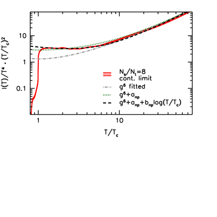
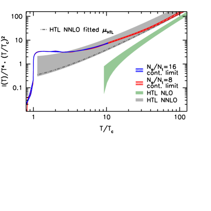
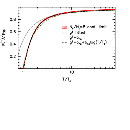
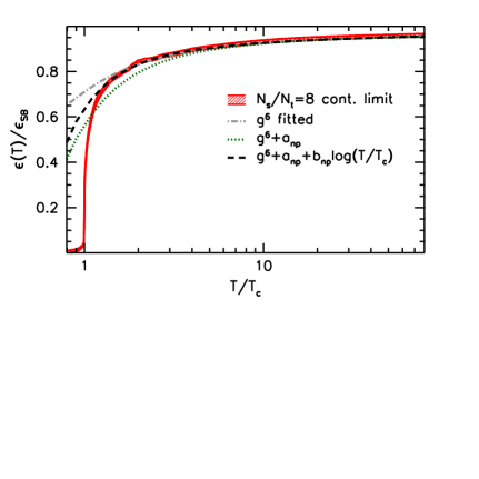
In the figure we also plot the perturbative formula plus a nonperturbative contribution using two simple functional forms and . Using the former ansatz we obtain , and the latter . We note that these parameters are rather sensitive to the variation of the lower endpoint of the fit interval, but the relatively small indicates (as it can be seen in the figure) that the low-temperature region is well described by the latter ansatz. Using thermodynamic relations the fitted perturbative formulae for the pressure and the energy density are also straightforward to calculate. In figure 4 we compare our small volume results to the so obtained predictions. Similar comparisons can be made for the case of the entropy density, too.
Tabulated data and the details of the present work will follow in a separate, longer publication.
Acknowledgments: The simulations have mainly been performed on the QPACE facility. The work was partially supported by the DFG grants SFB-TR55 and FO-502/1-2. Part of the calculation was running on the GPU cluster at the Eötvös University with the support from the European Research Council grant 208740 (FP7/2007-2013). The authors acknowledge the helpful comments from Axel Maas, Aleksi Kurkela, Marco Panero, Kari Rummukainen and York Schröder as well as the fruitful correspondence with Mike Strickland.
References
- [1] J. O. Andersen, M. Strickland and N. Su, Phys. Rev. Lett. 104, 122003 (2010); JHEP 1008, 113 (2010)
- [2] J. O. Andersen, L. E. Leganger, M. Strickland and N. Su, Phys. Lett. B 696 (2011) 468 arXiv:1009.4644 [hep-ph], arXiv:1103.2528 [hep-ph].
- [3] S. Borsanyi et al., JHEP 1011, 077 (2010) [arXiv:1007.2580 [hep-lat]].
- [4] K. Kajantie, M. Laine, K. Rummukainen and Y. Schroder, Phys. Rev. D 67, 105008 (2003)
- [5] G. Boyd, J. Engels, F. Karsch, E. Laermann, C. Legeland, M. Lutgemeier and B. Petersson, Phys. Rev. Lett. 75, 4169 (1995); Nucl. Phys. B 469, 419 (1996)
- [6] J. P. Blaizot, E. Iancu and A. Rebhan, Phys. Rev. D 68 (2003) 025011
- [7] J. Engels, J. Fingberg, F. Karsch, D. Miller and M. Weber, Phys. Lett. B 252, 625 (1990).
- [8] B. Beinlich, F. Karsch, E. Laermann and A. Peikert, Eur. Phys. J. C 6, 133 (1999)
- [9] M. Panero, Phys. Rev. Lett. 103, 232001 (2009)
- [10] S. Datta and S. Gupta, Phys. Rev. D 80, 114504 (2009)
- [11] T. Umeda et. al. [WHOT-QCD collaboration] Phys. Rev. D 79, 051501 (2009)
- [12] G. S. Bali and K. Schilling, Phys. Rev. D 47, 661 (1993)
- [13] M. Gockeler, R. Horsley, A. C. Irving, D. Pleiter, P. E. L. Rakow, G. Schierholz and H. Stuben, Phys. Rev. D 73, 014513 (2006)
- [14] M. Guagnelli, R. Sommer and H. Wittig [ALPHA collaboration], Nucl. Phys. B 535, 389 (1998)
- [15] G. Endrodi, Z. Fodor, S. D. Katz, K. K. Szabo, PoS LAT2007 (2007) 228.
- [16] Y. Chen et al., Phys. Rev. D 73, 014516 (2006)
- [17] F. Buisseret, Eur. Phys. J. C 68, 473 (2010)
- [18] N. Ishii, H. Suganuma and H. Matsufuru, Phys. Rev. D 66, 094506 (2002)
- [19] R. D. Pisarski, Prog. Theor. Phys. Suppl. 168, 276 (2007)
- [20] R. D. Pisarski, Phys. Rev. D 62, 111501 (2000)
- [21] K. I. Kondo, Phys. Lett. B 514, 335 (2001)