Statistics of gamma-ray point sources
below the Fermi detection limit

Abstract

An analytic relation between the statistics of photons in pixels and the number counts of multi-photon point sources is used to constrain the distribution of gamma-ray point sources below the Fermi detection limit at energies above 1 GeV and at latitudes below and above $30^{\circ}$. The derived source-count distribution is consistent with the distribution found by the Fermi collaboration based on the first Fermi point source catalogue. In particular, we find that the contribution of resolved and unresolved active galactic nuclei (AGN) to the total gamma-ray flux is below 20 to 25%. In the best fit model, the AGN-like point source fraction is $17\pm 2$%. Using the fact that the Galactic emission varies across the sky while the extra-galactic diffuse emission is isotropic, we put a lower limit of 51% on Galactic diffuse emission and an upper limit of 32% on the contribution from extra-galactic weak sources, such as star-forming galaxies. Possible systematic uncertainties are discussed.

Keywords: galaxies: active; gamma rays: diffuse background; gamma rays: general; methods: statistical; quasars: general

1 Introduction

Faint gamma-ray point sources cannot be detected individually, however their presence affects the statistics of photons across the sky. One can use the observed statistics of photons to infer some general properties about the population of point sources below the Fermi detection limit. The idea of using the statistics of photon counts or intensity maps in the study of faint point sources is familiar in radio and X-ray observations (e.g., Scheuer, 1957; Condon, 1974; Scheuer, 1974; Hasinger et al., 1993; Miyaji & Griffiths, 2002; Sołtan, 2011). A closely related subject is the use of extreme statistics to constrain the non-Gaussianity of cosmic microwave background data, e.g., Colombi et al. (2011) and references therein. In this paper, we extend the prior analysis (Slatyer & Finkbeiner, 2010) and use the points in cells statistics to understand the population of gamma-ray point sources.

In a larger context, the problem is to separate different sources of gamma-ray emission. The standard strategy is either to use templates (Dobler et al., 2010) that trace the sources or else to simulate the cosmic ray propagation and gamma-ray production using, e.g., Galprop (Strong et al., 2007, 2009). In this paper we would like to adopt a different methodology: we assume some general properties of the sources in order to obtain model-independent constraints on the contribution from these sources.

We separate the sources based on their statistical properties. In the paper we consider three sources of gamma-rays at high latitudes. The first source is a diffuse source that varies over large angles. The main contribution to this source comes from the Galactic diffuse emission ($\pi^{0}$ production, ICS photons, and bremsstrahlung) and, possibly, a population of faint Galactic point sources, such as millisecond pulsars (Faucher-Giguère & Loeb, 2010; Malyshev et al., 2010; 2010arXiv1011.5501S). We will call this source non-isotropic Galactic diffuse emission. It puts a lower limit on the actual Galactic emission.

The second source corresponds to an isotropic distribution of gamma-rays, i.e., the statistics of photons across the sky is consistent with the Poisson distribution for this source. The isotropic flux has contributions from the homogeneous part of the Galactic diffuse emission, from diffuse intergalactic emission (references can be found in Stecker & Venters, 2010), and from a population of very weak extragalactic sources that on average emit much less than one photon during the time of observation, such as star-forming galaxies (e.g., Pavlidou & Fields, 2002; Fields et al., 2010), starburst galaxies (Thompson et al., 2007), galaxy clusters (Berrington & Dermer, 2003), etc. The value of the isotropic emission puts an upper limit on the gamma-ray flux from very weak extra-galactic sources, as well as an upper limit on the contamination from cosmic rays (Abdo et al., 2010b).

The third source is a population of point sources modeled by a broken power-law source-count distribution. We assume that the point sources are distributed homogeneously over the sky. The statistics of photons coming from these point sources has a non-trivial form (derived in Appendix A) different from the Poisson statistics. These sources model a population of AGN-like point sources (Stecker et al., 1993; Padovani et al., 1993; Chiang et al., 1995; Stecker & Salamon, 1996; Mücke & Pohl, 2000; Abazajian et al., 2010; Neronov & Semikoz, 2011).

We note that in our approach it is impossible to separate the isotropic part of Galactic emission from the diffuse extragalactic background (EGB). Consequently, all results will be quoted either with respect to the total gamma-ray flux or in absolute values. We find that at high latitudes (below and above $30^{\circ}$) for energies above 1 GeV the contribution of AGN-like point sources (both resolved and unresolved) to the total gamma-ray flux is $17\%\pm 2$%, the contribution from Galactic diffuse emission is above 51% and the contribution from extra-galactic weak sources is below 32%. Using these values, we estimate that the contribution of unresolved AGN-like point sources to the EGB model in Abdo et al. (2010b) is below $\sim 25\%$, which is consistent with Abdo et al. (2010c).

The paper is organized as follows. In Section 2, we describe a general model and a fitting algorithm. In Section 3, we present an analysis of the Fermi data. Section 4 has discussion. In Appendix A, we derive the statistics of photons coming from a population of point sources. In Appendix B, we determine a model for non-isotropic Galactic diffuse emission. In Appendix C, we repeat the data analysis of Section 3 for different pixel sizes.

2 Model

In this section we describe the model that we later use to fit the Fermi gamma-ray data. At first, we present an analytic relation between the counts of photons in pixels and the statistics of point sources. Then we take into account the detector point spread function (PSF) and describe a model of Galactic diffuse gamma-ray emission. The model that we present in this section is rather general. An application of this analysis for the Fermi data is presented in Section 3.

2.1 Statistics of Photon Counts and Point Sources

We will assume a pixelation of the sphere with pixels of equal area. Usually a model of gamma-ray emission is represented in terms of the expected number $x_{p}$ of gamma-rays in pixel $p$. The problem is that the number and the positions of weak point sources are not known. The position of a point source can be found only by a “detection” of the source. However, if one is interested only in the total number of sources of a given flux, then a “detection” of sources is not necessary. In this paper, we use the statistics of photon counts in pixels, in order to find the source-count distribution of point sources without actual identification of the sources.

In order to find the statistics of photon counts in pixels we calculate the total number of pixels $n_{k}$ that contain $k$ photons. In this calculation, the information about the position of the pixels on the sky is not preserved, but the remaining information may be sufficient to constrain general properties of the population of sources. There are two competing conditions for this method to work. On the one hand, there should be sufficiently many pixels to determine the statistics of photon counts, while, on the other hand, the size of the pixels cannot be too small compared to the PSF, otherwise the statistics corresponding to the presence of point sources cannot be distinguished from non-isotropic diffuse emission.

If the total number of pixels is $N_{\rm pix}$ and $n_{k}$ is the observed number of pixels with $k$ photons, then we can estimate the probability to find $k$ photons in a pixel as

$$p_{k}=\frac{n_{k}}{N_{\rm pix}}.$$ (1)

For large $N_{\rm pix}$, the statistical uncertainty of $n_{k}$ is approximately $\sqrt{n_{k}}$ (there is a small correction due to the fact that the total number of pixels is fixed, i.e., the process is multinomial). If there are no point sources and all the emission comes from an isotropic diffuse source, then the probability distribution $p_{k}$ is the Poisson probability of getting $k$ photons given the mean rate. In the presence of point sources the probability distribution is more complicated than the Poisson distribution. In the context of X-ray point sources, the probability distribution is called a $P(D)$ distribution (or a $P(D)$ diagram) and is usually computed with the help of Monte Carlo simulations (e.g., Miyaji & Griffiths, 2002).

In this paper we find an analytic relation between the probability distribution of photon counts in pixels and the source-count distribution. We will use this relation to find a source-count distribution that has the best fit to the observed probability distribution determined in Equation (1).

In calculations we use the method of probability generating functions (an introduction can be found in, e.g., Hoel et al., 1971, Section 3.6). For a given discrete probability distribution $p_{k},\;k=0,1,2\ldots$, the corresponding generating function is defined as a power series in an auxiliary variable $t$

$$P(t)=\sum_{k=0}^{\infty}p_{k}t^{k}.$$ (2)

If the generating function $P(t)$ is known, then the probabilities $p_{k}$ can be found by picking the coefficient in front of $t^{k}$, or, equivalently, by differentiating with respect to $t$

$$p_{k}=\left.\frac{1}{k!}\frac{d^{k}P(t)}{dt^{k}}\right|_{t=0}.$$ (3)

An important property of probability generating functions is that a sum of two independent random variables corresponds to a product of the corresponding probability generating functions (Hoel et al., 1971). For example, if there are two independent sources of gamma-rays on the sky, e.g., Galactic and extragalactic, then the probability generating function for the photon counts with the two sources overlaid is given by the product of probability generating functions corresponding to the two sources (see Appendix A for more details).

Let $x_{m}$ denote the average number of sources inside a pixel that emit exactly $m$ photons during the time of observation. Using the sum-product property of probability generating functions (Hoel et al., 1971, Section 3.6), we derive in Appendix A the following relation between the probability generating function for the photon counts and the expected number $x_{m}$ of $m$-photon sources

$$\sum_{k=0}^{\infty}p_{k}t^{k}=\exp\left({\sum_{m=1}^{\infty}(x_{m}t^{m}-x_{m})}\right).$$ (4)

This formula provides an analytic relation between the expected numbers of $m$-photon sources and the statistics of photons in pixels. The probabilities $p_{k}$ to observe $k$ photons in a pixel are determined by expanding the right hand side of this equation and picking the coefficient in front of $t^{k}$.

If we substitute $t=e^{i\omega}$, then Equation (2) becomes a discrete Fourier transform analog of the probability characteristic functions (e.g., Hoel et al., 1971). The probability characteristic functions were extensively used in the study of radio point sources below detection limit (e.g., Scheuer, 1957). Similarly to probability generating functions, the characteristic function for a sum of two independent random variables corresponds to a product of the two characteristic functions.

The statistics of point sources can be described in terms of the differential source counts as a function of flux $S$, denoted by $dN/dS$. One of the simplest forms for the source-count distribution is a broken power-law

$$\frac{dN}{dS}\sim\left\{\begin{array}[]{l}S^{-n_{1}},\qquad S>S_{\rm break}\\ S^{-n_{2}},\qquad S<S_{\rm break},\end{array}\right.$$ (5)

where we have to require $n_{1}<2$ and $n_{2}>2$ in order to have a finite total flux.

Let $S$ be an average flux from a source (normalized to give the number of photons during the time of observation). Then the probability to observe $m$ photons from this source is

$$p_{m}(S)=\frac{S^{m}}{m!}e^{-S}.$$ (6)

If the sources are distributed isotropically, then the average number of $m$-photon sources inside a pixel is given by the Poisson probabilities for sources with flux $S$ to emit $m$ photons

$$x_{m}=\frac{\Omega_{\rm pix}}{4\pi}\int_{0}^{\infty}dS\frac{dN}{dS}(S)\frac{S^{m}}{m!}e^{-S},$$ (7)

where $\Omega_{\rm pix}$ is the angular area of the pixel.

2.2 PSF

In the case of non-zero PSF a source in some pixel may contribute gamma-rays to nearby pixels as well. In order to correctly estimate the number of point sources of a certain strength, we need to know how often a gamma-ray from a source in one pixel is detected in a different pixel.

We can represent the effect of the PSF as a smearing of a point source over some area, so that the flux from the point source is split between several pixels. We determine the average properties of the flux splitting from Monte Carlo simulations. In the simulation, we assume that the profile of the PSF is Gaussian. In order to calculate the average splitting, we put $n$ Gaussians at random positions on the sphere and integrate every Gaussian over the pixels to get a collection of fractions $f_{i},\;i=1,\ldots,N_{\rm pix}$, such that $f_{1}+f_{2}+\cdots=1$ (in practice, one can truncate at some minimal value of $f$). Denote by $\Delta n(f)$ the number of fractions for $n$ Gaussians that fall within $\Delta f$, then the average distribution of fractions is defined as

$$\rho(f)=\left.\frac{\Delta n(f)}{n\Delta f}\right|_{\Delta f\rightarrow 0,\>n\rightarrow\infty}.$$ (8)

This distribution is normalized as

$$\int f\rho(f)df=1.$$ (9)

The case of zero PSF corresponds to $\rho(f)=\delta(f-1)$. Sums over fractions are substituted by the integral $\int\rho(f)df$. In particular, the contribution of point sources with intrinsic flux between $S$ and $S+dS$ to the total number of $m$-photon sources is

$$dx_{m}=dN(S)\int df\rho(f)\frac{(fS)^{m}}{m!}e^{-fS}.$$ (10)

The expected number of $m$-photon sources inside a pixel including the effect of PSF is

$$x_{m}=\frac{\Omega_{\rm pix}}{4\pi}\int_{0}^{\infty}dS\frac{dN}{dS}(S)\int df\rho(f)\frac{(fS)^{m}}{m!}e^{-fS}.$$ (11)

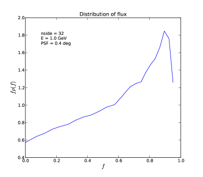
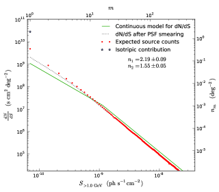
An example of the function $\rho(f)$ relevant for the data analysis in Section 3 is presented in Figure 1. If we rescale the integration variable $S$ in Equation (11) by $f$, then the effect of the PSF can be represented as a change of the source-count function

$$\frac{dN}{dS}(S)\longrightarrow\frac{d\tilde{N}}{dS}(S)=\int df\frac{\rho(f)}{f}\frac{dN}{dS}({S}/{f}).$$ (12)

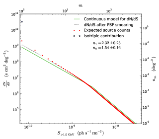
The apparent number of sources with small fluxes in $\frac{d\tilde{N}}{dS}$ is larger than the corresponding number of physical sources in $\frac{dN}{dS}$ due to contribution from point sources in nearby pixels, whereas the apparent number of sources with large fluxes is smaller due to loss of the flux to nearby pixels. One can see the effect of PSF in Figure 2 on the right. On the same figure, we also plot the expected number of $m$-photon sources for discrete $m$, derived from $\frac{d\tilde{N}}{dS}$.

2.3 The Model

In Equation (4), the probabilities $p_{k}$ and the average expected number of $m$-photon sources may depend on the position of the pixel. The quantity that we use is the averaged probability $p_{k}=\frac{n_{k}}{N_{\rm pix}}$, where $n_{k}$ is the number of pixels with $k$ photons. The generating function for averaged probabilities is given by

$$\sum_{k=0}^{\infty}{p}_{k}t^{k}=\frac{1}{N_{\rm pix}}\sum_{{\rm p}=1}^{N_{\rm pix}}{\rm exp}\left(\sum_{m=1}^{\infty}(x_{m}^{\rm p}t^{m}-x_{m}^{\rm p})\right).$$ (13)

This form of the generating function can be used when the distribution of sources is not isotropic or the exposure is non-uniform. If the exposure is sufficiently uniform, then we may assume that the distribution of extragalactic sources is independent of the pixel position and can be taken out of the sum over pixels. The diffuse emission corresponds to “one-photon” source density that depends on the pixel, $x_{\rm diff}({\rm p})$. Thus, the expression on the right-hand side of Equation (13) can be split into a product

$$\frac{1}{N_{\rm pix}}\sum_{{\rm p}=1}^{N_{\rm pix}}e^{x_{\rm diff}^{\rm p}t-x_{\rm diff}^{\rm p}+{\sum_{m=1}^{\infty}(x_{m}t^{m}-x_{m})}}=\left(\frac{1}{N_{\rm pix}}\sum_{{\rm p}=1}^{N_{\rm pix}}e^{x_{\rm diff}^{\rm p}t-x_{\rm diff}^{\rm p}}\right)\cdot e^{\sum_{m=1}^{\infty}(x_{m}t^{m}-x_{m})}$$ (14)

The second term in the product on the right hand side corresponds to the isotropic distribution of AGN-like point sources

$$P(t)={\rm exp}\left(\sum_{m=1}^{\infty}(x_{m}t^{m}-x_{m})\right),$$ (15)

while the first term corresponds to diffuse emission or, indistinguishably, one-photon sources

$$D(t)=\frac{1}{N_{\rm pix}}\sum_{{\rm p}=1}^{N_{\rm pix}}e^{x_{\rm diff}^{\rm p}t-x_{\rm diff}^{\rm p}}.$$ (16)

It is convenient to separate the diffuse emission into a non-isotropic part that puts a lower limit on Galactic diffuse emission and an isotropic part that consists of isotropic Galactic component and a possible population of weak extragalactic sources (additional to AGN-like sources)

$$x_{\rm diff}^{\rm p}=x_{\rm Gal}^{\rm p}+x_{\rm isotr}.$$ (17)

The main problem with the non-isotropic diffuse emission is a variability on large scales (on small scales the variability in Galactic emission is subdominant to Poisson noise and variability due to the presence of undetected point sources). In Appendix B we construct a model for the non-isotropic component $x_{\rm Gal}^{\rm p}$ that varies on large scales. We mask the known point sources and use low multipole spherical harmonics in order to filter out the small-scale variations while preserving the large-scale ones. We add a constant to $x_{\rm Gal}^{\rm p}$ so that ${\rm min}(x_{\rm Gal}^{\rm p})=0$. In the following, the non-isotropic component of diffuse emission is fixed. The corresponding generating function is

$$G(t)=\frac{1}{N_{\rm pix}}\sum_{{\rm p}=1}^{N_{\rm pix}}e^{x_{\rm Gal}^{\rm p}t-x_{\rm Gal}^{\rm p}}.$$ (18)

We denote the probability generating function for the isotropic emission as

$$I(t)=e^{x_{\rm isotr}t-x_{\rm isotr}}.$$ (19)

The total generating function for the probability distribution of photons in pixel is the product of the three components

$$\sum_{k=0}^{\infty}p_{k}t^{k}=P(t)\cdot G(t)\cdot I(t).$$ (20)

The parameters of the point-source distribution in Equation (5) and the level of the isotropic flux $x_{\rm isotr}$ are found from fitting the probability distribution given in Equation (20) to the observed probability distribution. The details of the fitting algorithm are presented in the next subsection.

This simple factorized form of the generating function is valid in every pixel. In general, this factorization is not possible if we take an average over pixels, unless at most one sources is non-isotropic and the other sources can be taken out of the average over pixels. The factorization leads to a significant simplification of calculations at the expense that, due to a variation in exposure, a part of isotropic EGB may be misinterpreted as a non-isotropic Galactic foreground. This effect is expected to be small, provided that the Fermi -LAT exposure is sufficiently uniform (Atwood et al., 2009). Another possible source of systematic uncertainty is that the distribution of galaxies in the local neighborhood of the Milky Way is non-uniform and a part of emission from these galaxies can be misinterpreted as Galactic emission.

2.4 Fitting Algorithm

The algorithm has two main parts:

1. Determine the non-isotropic part $x_{\rm Gal}^{\rm p}$ of Galactic diffuse emission. We mask the bright point sources and use low multipoles of spherical harmonics to find the variable part of the remaining flux (Appendix B). Then we add a constant such that ${\rm min}(x_{\rm Gal}^{\rm p})=0$. In the following $x_{\rm Gal}^{\rm p}$ is fixed, i.e. we do not vary this component in fitting the pixel counts.

2. Use pixel counts to find $x_{\rm isotr}$ and $dN/dS$. The source-count distribution has four parameters: normalization, break, and two indices. Together with the level of isotropic contribution, $x_{\rm isotr}$, this gives five fitting parameters which we denote by $\alpha=(A,S_{\rm break},n_{1},n_{2},x_{\rm isotr})$, where $A$ denotes the normalization in the source-count distribution in Equation (5).

The model prediction for the pixel counts $\nu_{k}(\alpha)$ is determined by multiplying the right-hand side of Equation (20) by $N_{\rm pix}$

$$N_{\rm pix}\cdot P(t)\cdot G(t)\cdot I(t)=\sum_{k=0}\nu_{k}(\alpha)t^{k}.$$ (21)

The expected pixel counts $\nu_{k}(\alpha)$ are found by expanding the left-hand side of this equation in powers of $t$ and picking the coefficient in front of $t^{k}$. Given the observed number of pixels $n_{k}$ with $k$ photons, the likelihood of $\nu_{k}(\alpha)$ is estimated by the Poisson probability

$$L_{k}=\frac{\nu_{k}^{n_{k}}}{n_{k}!}e^{-\nu_{k}}.$$ (22)

The overall likelihood of the model is estimated as

$$L(\alpha)=\prod_{k}\frac{\nu_{k}(\alpha)^{n_{k}}}{n_{k}!}e^{-\nu_{k}(\alpha)}.$$ (23)

Here the product is over the number of photons $k$, while the data are represented by the number of pixels $n_{k}$ that contain $k$ photons. This is different from a usual coordinate space fit of maps, where the product is over pixels and the data are the number of photons $k_{p}$ in a pixel $p$.

We use this likelihood function to find the best-fit parameters $\alpha_{*}$ for a given set of observed pixel counts $n_{k}$. The significance of deviation of $\alpha$ from $\alpha_{*}$ can be estimated as

$$\frac{\sigma(\alpha)^{2}}{2}=\ln L(\alpha_{*})-\ln L(\alpha).$$ (24)

In the case of large counts the likelihood is well approximated by the Gaussian distribution and $\sigma(\alpha)$ is the deviation in sigma values.

3 Data analysis

Figure 1: Average distribution of flux among pixels from Gaussian sources at random positions. The width of the Gaussian corresponds to the average point spread function for front-converted gamma-rays with energies between 1 GeV and 300 GeV. The pixels are determined in HEALPix (Górski et al., 2005) with ${\rm nside=32}$. $x$-axis: fraction of the flux, $y$-axis: density of pixels as a function of $f$ (cf., Equation (8)) multiplied by the flux fraction. The fractions are computed by taking 50,000 Gaussian distributions at random positions on the sphere. The area under the curve corresponds to the total flux equal to 1.

Figure 2: Left plot: $n_{k}$ is the number of pixels with $k$ photons, the red dots correspond to pixel counts derived from Fermi data, the errors bars are equal to $\sqrt{n_{k}}$. We consider three sources: AGN-like point sources (blue dotted line), isotropic Poisson contribution (brown dashed line), and non-isotropic Galactic diffuse emission (black dash-dotted line). Note, that the total model on this plot is not the sum of the components, the corresponding generating function of the PDF is a product of the generating functions in Equation (20). $N_{\rm points}$ corresponds to the number of points on the $x$-axis that we have used for fitting, $k<500$. Right plot: green solid line is the physical model for the AGN-like source counts, blue dotted line is the source counts in pixels in the presence of PSF (Equation (12)), points represent expected number of $m$-photon sources per ${\rm deg^{2}}$ as defined in Equation (11), blue star is the value of the isotropic flux.

We consider 11 months of Fermi data (August 4, 2008 - July 4, 2009) that were used for the first Fermi point-source catalog (Abdo et al., 2010a) and for the Fermi analysis of the source-count distribution (Abdo et al., 2010c).

In order to reduce the PSF, we use front-converted gamma-rays, i.e., the gamma-rays converted in the front part of the Fermi-LAT tracker (Atwood et al., 2009), with energies between 1 GeV and 300 GeV. The corresponding (quadratic) average of the PSF is $0.4^{\circ}$. For pixelation of data, we use HEALPix (Górski et al., 2005) with the pixelation parameter nside = 32, which corresponds to pixel size about $2$ degrees. We mask the galactic plane within 30 degrees in latitude. The number of pixels outside of the mask is $N_{\rm pix}=6178$ and the number of photons is 152,143.

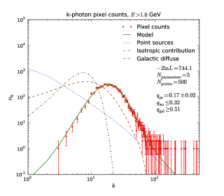
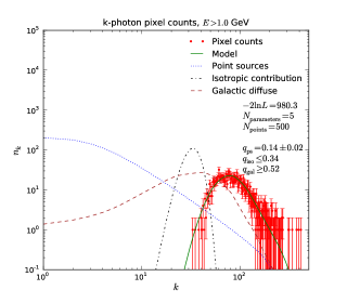
The distribution of pixel counts is presented in Figure 2 on the left. We model this distribution by a combination of three components: non-isotropic Galactic diffuse emission derived in Appendix B, isotropic distribution of photons, and the distribution of AGN-like point sources described in Section 2.3. The best-fit models for the isotropic flux and the AGN-like point sources are presented in Figure 2 on the right.

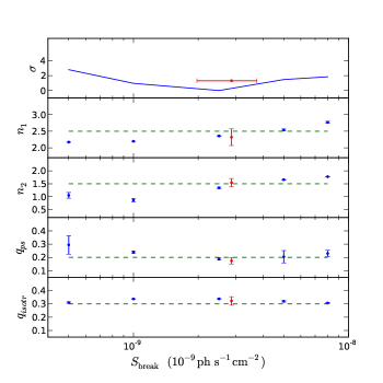
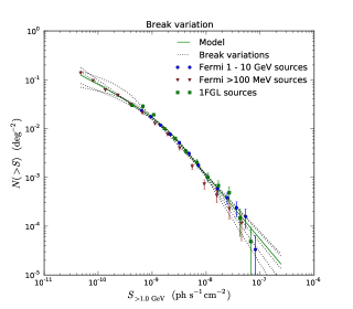
In fitting we consider pixel counts $n_{k}$ with $k<500$, i.e., the number of data points is $N_{\rm points}=500$. We use $\ell_{\rm max}=20$ for the Galactic diffuse emission model. The sampling is performed with Metropolis-Hastings Markov Chain Monte Carlo method with 1500 steps. The average model is presented in Figure 2 and compared with Fermi models in Table 1. We find that the position of the break is almost a flat direction. The results of fitting with a set of fixed break positions are presented in Figure 3.

Figure 3: Results of fitting the AGN-like source-count distribution for fixed positions of the break. The significance of deviation is determined from Equation (24) as $\sigma=\sqrt{2\Delta\ln L}$. $n_{1}$ and $n_{2}$ are the indices above and below the break for differential source-count distribution, $q_{\rm ps}$ is the fractional contribution from AGN-like point sources, $q_{\rm isotr}$ is the fractional contribution from an isotropic source (it provides an upper limit on the extra-galactic isotropic contribution additional to AGN-like point sources). Red dots correspond to the model used in Figure 2. Green dashed lines provide reference values: $n_{1}=2.5$, $n_{2}=1.5$, $q_{\rm ps}=0.2$, and $q_{\rm isotr}=0.3$.

Table 1: Comparison with Fermi Results (Abdo et al., 2010c).

Analysis	$n_{1}$	$n_{2}$	$S_{\rm break}^{a}$
This work	$2.31\pm 0.25$	$1.54\pm 0.16$	$2.9\pm 0.9$
Fermi $>100$ MeV	$2.44\pm 0.11$	$1.58\pm 0.08$	$2.8\pm 0.5^{b}$
Fermi 1 - 10 GeV	$2.38^{+0.15}_{-0.14}$	$1.52^{+0.8}_{-1.1}$	$\rm 2.3\pm 0.6$

^a In units of $10^{-9}{\rm ph\>s^{-1}cm^{-2}}$.
^b Rescaled from the break in Abdo et al. (2010c) according to energy spectrum $\sim E^{-2.4}$.

We find that the contribution of point sources to the gamma-ray flux is $(17\pm 2)\%$. This fraction is obtained by integrating the best-fit source-count model presented in Figure 2 and in Table 1 from zero to infinity. This fraction is not model independent, i.e., it may change for different shapes of the source-count function used in fitting, but, provided that the broken power-law source-counts distribution gives a good fit to the data, we do not expect a large systematic uncertainty due to the change in the shape of the fitting function. In part this can be justified by looking at the models with fixed positions of the break: most of the models in Figure 3 have the point-source fraction $q_{\rm ps}\lesssim 0.25$.

At smaller position of the break the contribution of point sources becomes larger ($q_{\rm ps}\sim 0.3$ for the left point in Figure 3) but the fit has smaller likelihood. It would be interesting to estimate constraints on models involving high redshift AGNs to explain the unresolved part of the EGB (e.g., Abazajian et al., 2010; Neronov & Semikoz, 2011) using the statistics of photon counts.

We can also put an approximate lower bound of 51% on Galactic diffuse emission, and an approximate upper bound of 32% on isotropic emission consistent with Poisson statistics. In terms of the absolute flux values, the total gamma-ray flux above 1 GeV for $|b|>30^{\circ}$ is $F_{\rm tot}=1.75\times 10^{-6}\>{\rm s^{-1}cm^{-2}sr^{-1}}$, the diffuse Galactic flux is $F_{\rm Gal}>8.8\times 10^{-7}\>{\rm s^{-1}cm^{-2}sr^{-1}}$, the isotropic component of the flux is $F_{\rm isotr}=(5.6\pm 0.6)\times 10^{-7}\>{\rm s^{-1}cm^{-2}sr^{-1}}$, the flux from AGN-like point sources with $dN/dS$ parameters given in Table 1 and in Figure 2 is $F_{\rm PS}=(3.0\pm 0.4)\times 10^{-7}\>{\rm s^{-1}cm^{-2}sr^{-1}}$.

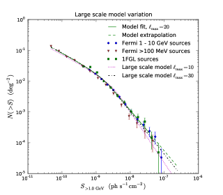
Using this value of the total flux from AGN-like point sources, we can estimate the gamma-ray flux from undetected sources. The total flux in the energy range 1 - 100 GeV from point sources at $|b|>30^{\circ}$ detected by Fermi (Abdo et al., 2010a) is $F_{\textsl{Fermi}\>\rm AGN}=2.1\times 10^{-7}\>{\rm s^{-1}cm^{-2}sr^{-1}}$. Consequently, the flux from undetected AGN-like point sources above $30^{\circ}$ can be estimated as $F_{\rm unres\>AGN}=0.9\times 10^{-7}\>{\rm s^{-1}cm^{-2}sr^{-1}}$. This value is reasonable, since from Figure 4 it follows that the detected point sources give a good approximation to the best-fit distribution of sources down to fluxes below the break in $N(S)$, while the contribution of point sources to the gamma-ray background is saturated around the break. The extragalactic diffuse emission can be estimated from the model presented in Abdo et al. (2010b). In this model, the EGB flux above 1 GeV is $F_{\rm EGB}\approx 4\times 10^{-7}\>{\rm s^{-1}cm^{-2}sr^{-1}}$. The contribution of unresolved AGN’s to this EGB flux is about $23\%$. This value is consistent with the estimations in Abdo et al. (2010c). We would like to stress that our analysis is different from Abdo et al. (2010c). We do not count any sources, but rather do a “blind” statistical analysis. The consistency of results may serve as a non-trivial check of both methods.

Figure 4: Left plot: different lines correspond to different models for Galactic diffuse emission of gamma-rays corresponding to $\ell_{\rm max}=10,\>20,\>30$ (Appendix B). Solid green line corresponds to the range of photon counts (1 to 500) used in fitting. Dashed green line is the extrapolation of the model. Magenta triangles correspond to total source counts found by Fermi collaboration above 100 MeV (right plot in Figure 9 of Abdo et al., 2010c) with flux rescaled assuming energy density spectrum $\sim E^{-2.4}$. Blue circles correspond to sources found by the Fermi collaboration in $1-10$ GeV energy bin (center plot in Figure 17 of Abdo et al. (2010c)). Green squares correspond to $1-100$ GeV flux for sources in the first Fermi catalog (Abdo et al., 2010a). Right plot: models with different fixed positions of the break presented in Figure 3.

4 Discussion

One of the most interesting problems in gamma-ray astrophysics is to understand the origin of EGB flux, which is defined as the total gamma-ray flux minus the contribution from resolved point sources, minus the Galactic foreground (Abdo et al., 2010b). In general, we can separate the sources of diffuse EGB into two big classes: non-Poisson sources and Poisson-like sources. In the first case, the contribution comes from sources below detection limit that may emit several photons during the observation time, these are the AGN-like point sources (e.g., Padovani et al., 1993; Chiang et al., 1995; Stecker & Salamon, 1996; Abazajian et al., 2010; Neronov & Semikoz, 2011). In this case the statistics of photon counts in pixels across the sky will be different from Poisson statistics due to correlation among photons coming from the same point source. In the second case, there is a large number of sources emitting on average much fewer than one photon during the observation time, e.g., star-forming and star-burst galaxies (Pavlidou & Fields, 2002; Thompson et al., 2007; Fields et al., 2010). The statistics of photons in this case will be very close to Poisson statistics.

These two possibilities are relatively hard to separate based only on energy spectrum arguments (see, however, Abazajian et al., 2010; Stecker & Venters, 2010; Neronov & Semikoz, 2011). Alternatively, one can use a correlation between gamma-ray emission and multi-wavelength emission from AGNs (Urry & Padovani, 1995; Mücke & Pohl, 2000; Abdo et al., 2010d; Angelakis et al., 2010; Li & Cao, 2011) together with AGN population studies (e.g., Padovani & Giommi, 1995; Hopkins et al., 2007; Padovani et al., 2007; Rigby et al., 2008; Hodge et al., 2009; Smolčić et al., 2009) to infer the AGN contribution to gamma-ray background.

In this paper we show that the statistics of photons in pixels can also be used to constrain the distribution of point sources below the detection limit. We find that there is a slight preference for two populations of point sources: the AGN-like point sources with a break at relatively high flux and a population of faint sources such as star-forming galaxies rather than a single population of AGN-like point sources with a break at a smaller flux. This statement is insensitive to the energy spectrum since we use the integrated flux above 1 GeV but it may depend on the form of the function used to fit the point source number counts. Possible sources of systematic uncertainty include the source smearing due to PSF, non-isotropic Galactic diffuse emission, non-isotropic emission (on large scales) from nearby galaxies, and non-homogeneous exposure. The interpretation of the point-source number counts may also be affected by clustering of sources on scales smaller than the PSF.

A stronger constrain on the population of gamma-ray point sources may come from an unpixelized analysis of the data. In this more general analysis, the likelihood of a model depends on the full gamma-ray data (positions on the sky, energy, arrival time) rather than the counts of gamma-rays in pixels. This likelihood would have the form of an integral over flux times the source number counts, times an integral over all possible positions of the sources on the sky. The photon counts approximation is simpler computationally and already gives rough constraints on the source population, while the full unbinned analysis may provide stronger constraints at the expense of computational complexity. Examples of unbinned analysis using some part of gamma-ray data include the gamma-ray two-point correlation function (e.g., Ave et al., 2009; Geringer-Sameth & Koushiappas, 2010), angular power spectrum (Ando & Komatsu, 2006; Hensley et al., 2010), nearest neighbor statistics (Sołtan, 2011), etc.

We also believe that the techniques of generating functions in the study of photon counts statistics, known for some time in radio and X-ray observations, may have further important applications in data analysis of current and future radio, IR, X-ray, and gamma-ray observations.

Acknowledgments.

The authors are thankful to Kevork Abazajian, Marko Ajello, Jo Bovy, Christopher Kochanek, Jennifer Siegal-Gaskins, Tracy Slatyer, Tonia Venters, and Itay Yavin for stimulating discussions and useful comments. We are also thankful to Ilias Cholis for the help in selecting the Fermi gamma-ray data. This work is supported in part by the Russian Foundation of Basic Research under Grant No. RFBR 10-02-01315 (D.M.), by the NSF Grant No. PHY-0758032 (D.M.), by Packard Fellowship No. 1999-1462 (D.M.), by NASA grant NNX08AJ48G (D.W.H.), and by the NSF grant AST-0908357 (D.W.H.). Some results in this paper have been obtained using the HEALPix package (Górski et al., 2005).

Appendix A Derivation of statistics

In this Appendix we derive the photon counts statistics in the presence of point sources. The derivation is based on the following well known property of generating functions for probabilities: the generating function of a sum of two independent sources is the product of the corresponding generating functions (e.g., Hoel et al., 1971, Section 3.6). Indeed, consider a box where we can put red balls with probabilities $p_{k}$, $k=1,\>2,\>3\ldots$, and blue balls with corresponding probabilities $q_{k}$, $k=1,\>2,\>3\ldots$, then the probability to find $k$ balls of any color is

$$r_{k}=\sum_{k^{\prime}=0}^{k}p_{k^{\prime}}q_{k-k^{\prime}},\qquad k=1,\>2,\>3\ldots$$ (A1)

The last equation is the rule for multiplication of polynomials or power series. Let

$$R(t)=\sum_{k}r_{k}t^{k},\qquad P(t)=\sum_{k}p_{k}t^{k},\qquad Q(t)=\sum_{k}q_{k}t^{k},$$ (A2)

then

$$R(t)=P(t)\cdot Q(t).$$ (A3)

As before, denote the probability to observe $k$ photons in a pixel by $p_{k}$. The corresponding generating function is

$$P(t)=\sum_{k}p_{k}t^{k}.$$ (A4)

The knowledge of the generating function is equivalent to the knowledge of all $p_{k}$, provided that every $p_{k}$ can be found from $P(t)$ by picking the term in front of $t^{k}$.

We will now derive the generating function for probabilities to observe $k$ photons from a collection of point sources. Denote by $x_{m}$ the average number of point sources inside a pixel that emit exactly $m$ photons during the time of observation. We assume that the probability to find $n_{m}$ $m$-photon sources in a pixel is given by the Poisson statistics

$$p_{n_{m}}(x_{m})=\frac{x_{m}^{n_{m}}}{n_{m}!}e^{-x_{m}},$$ (A5)

then the probability to find $k$ photons from $m$-photon sources is

$$p^{(m)}_{k}=\left\{\begin{array}[]{ll}p_{n_{m}}(x_{m}),&\text{if $k=m\cdot n_{m}$ for some $n_{m}$};\\ 0,&\text{otherwise}.\end{array}\right.$$ (A6)

The corresponding probability generating function is

$$P^{(m)}(t)=\sum_{k}p_{k}t^{k}=\sum_{n_{m}}t^{m\cdot n_{m}}\frac{x_{m}^{n_{m}}}{n_{m}!}e^{-x_{m}}=e^{x_{m}t^{m}-x_{m}}.$$ (A7)

The generating function of probabilities $p_{k}$ to observe $k$ photons from any sources is the product of the generating functions for every $m$

$$\sum_{k=0}^{\infty}p_{k}t^{k} = \prod_{m=1}^{\infty}e^{x_{m}t^{m}-x_{m}}$$ (A8)

$$= {\rm exp}\left(\sum_{m=1}^{\infty}(x_{m}t^{m}-x_{m})\right).$$

If we denote $t=e^{2\pi i\omega}$ and

$$\tilde{P}(\omega) = \sum_{k=0}^{\infty}p_{k}e^{2\pi i\omega k},$$ (A9)

$$\tilde{X}(\omega) = \sum_{m=0}^{\infty}x_{m}e^{2\pi i\omega m},$$ (A10)

then Equation (A8) can be represented as

$$\tilde{P}(\omega)=e^{\tilde{X}(\omega)-\tilde{X}(0)},$$ (A11)

which is the discrete Fourier transform analog of characteristic functions considered in, e.g., Scheuer (1957).

Appendix B Non-isotropic Galactic diffuse emission

In this appendix, we describe a model for the non-isotropic Galactic diffuse emission. This signal is “filtered” by low multipoles of the gamma-ray data. In this approach, the homogeneous part of Galactic emission is indistinguishable from extragalactic flux. Also some part of extragalactic emission from galaxies and galaxy clusters close to Milky Way may lead to a signal that varies over the sky and can be misinterpreted as non-isotropic Galactic emission. However, the majority of extragalactic emission comes from higher redshifts where the distribution of extragalactic sources is sufficiently uniform on large scales.

Figure 5: Blue line (upper): angular power spectrum of gamma-ray data with $|b|>30^{\circ}$. Red line (lower): same as the blue line, but with additional masking of Fermi gamma-ray point sources (Figure 6). The normalization is chosen such that for the Poisson noise $\langle C_{l}\rangle=1$ (constant green line). $C_{l}$’s below $\ell\sim 10$ are dominated by the variation in Galactic diffuse emission on large scales. Constant $C_{l}$’s above $\ell=10$ are due to contribution of point sources. Decay of $C_{l}$’s above $\ell\sim 100$ for the blue line is due to detector PSF. In our case $\langle\rm PSF\rangle\approx 0.4^{\circ}$, which corresponds to $\ell\gtrsim 400$. A smoothed model for large-scale structure distribution is obtained by spherical harmonics decomposition up to $\ell=20$, the corresponding map of the model is presented in Figure 6.

Figure 6: Sky maps for photon counts and for a Galactic diffuse emission model derived from the photon counts by using the spherical harmonics decomposition with $l\leq 20$ (Equation (B2)). Residuals are in sigma values: $\frac{|{\rm model}-{\rm data}|}{\sqrt{{\rm model}}}$.

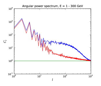
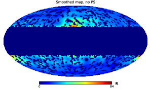
In Figure 5, we plot the angular power spectrum for the data at high latitudes ($|b|>30^{\circ}$) before and after masking the point sources in the first Fermi catalog (Abdo et al., 2010a). The angular power spectrum is

$$C_{l}=\frac{1}{2l+1}\sum_{m}|a_{lm}|^{2},$$ (B1)

where $a_{lm}$’s are the spherical harmonics coefficients of $f(p)\cdot m(p)$, where $f(p)$ is the number of photon counts inside pixel $p$ and $m(p)$ is the mask function. The mask function is equal to one (zero) for $|b|>30^{\circ}$ ($|b|<30^{\circ}$). In the case of masked point sources, we also have $m(p)=0$ when a Fermi point source is inside the pixel or within two PSF from the boundary of the pixel. We also subtract the average of the data within the unmasked region in order to avoid a non-trivial contribution from a constant source inside the window. We choose the normalization such that for the Poisson noise $\langle C_{l}\rangle=1$.

Figure 7: Photon counts vs smooth model with Fermi point sources subtracted. The Galactic diffuse emission model is obtained by taking the spherical harmonics of the data with $\ell\leq 20$. The model photon counts are derived from the probability generating function in Equation (16) with $x_{\rm diff}$ given in Equation (B2).

The algorithm for estimating the component that varies on large scales is as follows:

1. Calculate the $a_{lm}$’s inside a window larger than needed (in order to avoid edge effects). We use $|b|>20^{\circ}$ for the data above $30^{\circ}$. We also fill in the pixels with point sources by the average of nearest neighbors.

2. The large-scale distribution of gamma-rays is defined as

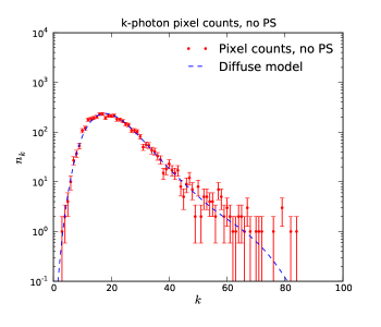
   $$x_{\rm diff}(p)=A\sum_{l=0}^{l_{\rm max}}\sum_{m=-l}^{l}a_{lm}Y_{lm}(p)+B,$$ (B2)

   where we find the coefficients $A$ and $B$ from the best fit of the diffuse model to the photon counts in the pixels without point sources (see Figure 7).

3. We represent $B=B_{\rm min}+x_{\rm isotr}$ so that

   $$x_{\rm Gal}(p)=A\sum_{l=0}^{l_{\rm max}}\sum_{m=-l}^{l}a_{lm}Y_{lm}(p)+B_{\rm min}$$ (B3)

   is non-negative for $|b|>30^{\circ}$. In fitting to full data, $A$ and $B_{\rm min}$ are fixed, while $x_{\rm isotr}$ is allowed to vary together with parameters describing the AGN-like point sources.

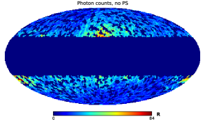
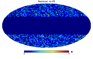
An example of the diffuse emission model $x_{\rm diff}(p)$ for $l_{\rm max}=20$ is presented in the middle plot of Figure 6. The top plot represents the counts of photons in pixels inside the window $|b|>30^{\circ}$ with masked Fermi gamma-ray point sources. The bottom plot represents the deviation of the model from the data in “sigma” values. In Figure 4 we study the effect of changing $l_{\rm max}=10,20,30$. The difference is rather small, i.e., already $l_{\rm min}=10$ captures the large-scale distribution of gamma-rays reasonably well.

Appendix C Variation of pixel size

In the data analysis in Section 3, we use the pixel size of about $2^{\circ}$ corresponding to HEALPix parameter nside = 32. In this appendix, we repeat the analysis of Section 3 for different sizes of pixels, in particular we consider nside = 64 and nside = 16 corresponding to pixel sizes $1^{\circ}$ and $4^{\circ}$ respectively.

Figure 8: Same as in Figure 2 but with the pixel size of about $1^{\circ}$ corresponding to HEALPix parameter nside = 64.

Figure 9: Comparison with Fermi source counts (Abdo et al., 2010a, c) in the case of analysis with HEALPix parameter nside = 64 (Figure 8).

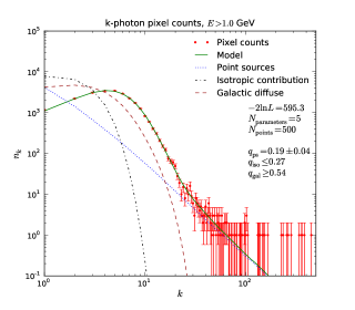
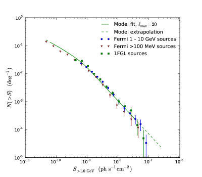
The results for nside = 64 are presented in Figure 8. The total number of pixels inside the window below and above $30^{\circ}$ in latitude is about 25,000, i.e., the statistics of pixel counts is relatively good, but the effect of PSF becomes more significant than in the case of nside = 32. For PSF = $0.4^{\circ}$, less than about 60% of the flux from a source can be inside one pixel. In particular, one can note that the number of sources with small fluxes is about two times larger than in the input model. Nonetheless, in the case of nside = 64 the best-fit model is similar to nside = 32 case. The position of the break, $S_{\rm break}=1.1\times 10^{-9}{\rm ph\>s^{-1}cm^{-2}}$, is somewhat lower than the values in Table 1 but the overall source count distribution (Figure 9) is consistent with the source counts found by Fermi collaboration (Abdo et al., 2010a, c).

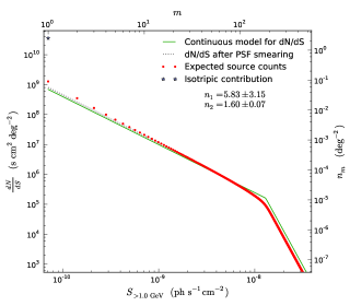
The results of fitting for nside = 16 are presented in Figure 10. In this case, the PSF can be neglected. However, the number of pixels inside the window is only about 1,500. As one can see on the left side of Figure 10, the error bars are rather large and the photon counts in most of the pixels are dominated by the contribution from diffuse emission. As a result, our method is not sensitive to the contribution from point sources for nside = 16. In particular, the MCMC is dominated by models with large $S_{\rm break}$. The best fit value $S_{\rm break}=1.3\times 10^{-8}{\rm ph\>s^{-1}cm^{-2}}$ is an order of magnitude larger than the values in Table 1. The reason is that models with large $S_{\rm break}$ have a comparable likelihood to the models with small $S_{\rm break}$ but there are many more ways to choose a large $S_{\rm break}$.

We conclude that our method is relatively robust to the change of pixel size: the cases of nside = 32 and nside = 64 give very similar results, unless the number of pixels is not sufficient to draw any conclusion about the statistics of sources, as in the case of nside = 16.

Figure 10: Same as in Figure 2 but with the pixel size of about $4^{\circ}$ corresponding to HEALPix parameter nside = 16.

References

- Abazajian et al. (2010) Abazajian, K. N., Blanchet, S., & Harding, J. P. 2010, arXiv:1012.1247
- Abdo et al. (2010a) Abdo, A. A., et al. 2010a, ApJS, 188, 405
- Abdo et al. (2010b) —. 2010b, Physical Review Letters, 104, 101101
- Abdo et al. (2010c) —. 2010c, ApJ, 720, 435
- Abdo et al. (2010d) —. 2010d, ApJ, 716, 30
- Ando & Komatsu (2006) Ando, S., & Komatsu, E. 2006, Phys. Rev. D, 73, 023521
- Angelakis et al. (2010) Angelakis, E., Fuhrmann, L., Nestoras, I., Zensus, J. A., Marchili, N., Pavlidou, V., & Krichbaum, T. P. 2010, arXiv:1006.5610
- Atwood et al. (2009) Atwood, W. B., et al. 2009, ApJ, 697, 1071
- Ave et al. (2009) Ave, M., et al. 2009, J. Cosmology Astropart. Phys, 7, 23
- Berrington & Dermer (2003) Berrington, R. C., & Dermer, C. D. 2003, ApJ, 594, 709
- Chiang et al. (1995) Chiang, J., Fichtel, C. E., von Montigny, C., Nolan, P. L., & Petrosian, V. 1995, ApJ, 452, 156
- Colombi et al. (2011) Colombi, S., Davis, O., Devriendt, J., Prunet, S., & Silk, J. 2011, arXiv:1102.5707
- Condon (1974) Condon, J. J. 1974, ApJ, 188, 279
- Dobler et al. (2010) Dobler, G., Finkbeiner, D. P., Cholis, I., Slatyer, T., & Weiner, N. 2010, ApJ, 717, 825
- Faucher-Giguère & Loeb (2010) Faucher-Giguère, C., & Loeb, A. 2010, J. Cosmology Astropart. Phys, 1, 5
- Fields et al. (2010) Fields, B. D., Pavlidou, V., & Prodanović, T. 2010, ApJ, 722, L199
- Geringer-Sameth & Koushiappas (2010) Geringer-Sameth, A., & Koushiappas, S. M. 2010, arXiv:1012.1873
- Górski et al. (2005) Górski, K. M., Hivon, E., Banday, A. J., Wandelt, B. D., Hansen, F. K., Reinecke, M., & Bartelmann, M. 2005, ApJ, 622, 759
- Hasinger et al. (1993) Hasinger, G., Burg, R., Giacconi, R., Hartner, G., Schmidt, M., Trumper, J., & Zamorani, G. 1993, A&A, 275, 1
- Hensley et al. (2010) Hensley, B. S., Siegal-Gaskins, J. M., & Pavlidou, V. 2010, ApJ, 723, 277
- Hodge et al. (2009) Hodge, J. A., Zeimann, G. R., Becker, R. H., & White, R. L. 2009, AJ, 138, 900
- Hoel et al. (1971) Hoel, P. G., Port, S. C., & Stone, C. J. 1971, Introduction to Probability Theory (Boston, MA: Houghton Mifflin)
- Hopkins et al. (2007) Hopkins, P. F., Richards, G. T., & Hernquist, L. 2007, ApJ, 654, 731
- Li & Cao (2011) Li, F., & Cao, X. 2011, arXiv:1103.4545
- Malyshev et al. (2010) Malyshev, D., Cholis, I., & Gelfand, J. D. 2010, ApJ, 722, 1939
- Miyaji & Griffiths (2002) Miyaji, T., & Griffiths, R. E. 2002, ApJ, 564, L5
- Mücke & Pohl (2000) Mücke, A., & Pohl, M. 2000, MNRAS, 312, 177
- Neronov & Semikoz (2011) Neronov, A., & Semikoz, D. V. 2011, arXiv:1103.3484
- Padovani et al. (1993) Padovani, P., Ghisellini, G., Fabian, A. C., & Celotti, A. 1993, MNRAS, 260, L21
- Padovani & Giommi (1995) Padovani, P., & Giommi, P. 1995, ApJ, 444, 567
- Padovani et al. (2007) Padovani, P., Giommi, P., Landt, H., & Perlman, E. S. 2007, ApJ, 662, 182
- Pavlidou & Fields (2002) Pavlidou, V., & Fields, B. D. 2002, ApJ, 575, L5
- Rigby et al. (2008) Rigby, E. E., Best, P. N., & Snellen, I. A. G. 2008, MNRAS, 385, 310
- Scheuer (1957) Scheuer, P. A. G. 1957, in Proceedings of the Cambridge Philosophical Society, Vol. 53, Proceedings of the Cambridge Philosophical Society, 764–773
- Scheuer (1974) Scheuer, P. A. G. 1974, MNRAS, 166, 329
- Slatyer & Finkbeiner (2010) Slatyer, T. R., & Finkbeiner, D. P. 2010, MNRAS, 405, 1777
- Smolčić et al. (2009) Smolčić, V., et al. 2009, ApJ, 696, 24
- Sołtan (2011) Sołtan, A. M. 2011, arXiv:1101.0256
- Stecker & Salamon (1996) Stecker, F. W., & Salamon, M. H. 1996, ApJ, 464, 600
- Stecker et al. (1993) Stecker, F. W., Salamon, M. H., & Malkan, M. A. 1993, ApJ, 410, L71
- Stecker & Venters (2010) Stecker, F. W., & Venters, T. M. 2010, arXiv:1012.3678
- Strong et al. (2009) Strong, A. W., Moskalenko, I. V., Porter, T. A., Jóhannesson, G., Orlando, E., & Digel, S. W. 2009, arXiv:0907.0559
- Strong et al. (2007) Strong, A. W., Moskalenko, I. V., & Ptuskin, V. S. 2007, Annual Review of Nuclear and Particle Science, 57, 285
- Thompson et al. (2007) Thompson, T. A., Quataert, E., & Waxman, E. 2007, ApJ, 654, 219
- Urry & Padovani (1995) Urry, C. M., & Padovani, P. 1995, PASP, 107, 803