SMOOTHED EXTREME VALUE ESTIMATORS

OF NON-UNIFORM POINT PROCESSES BOUNDARIES

WITH APPLICATION TO STAR-SHAPED SUPPORTS ESTIMATION

Stéphane Girard⁽¹⁾ and Ludovic Menneteau⁽²⁾

⁽¹⁾ INRIA Rhône-Alpes, ⁽²⁾ Université Montpellier 2

Abstract: We address the problem of estimating the edge of a bounded set in $\mathbb{R}^{d}$ given a random set of points drawn from the interior. Our method is based on a transformation of estimators dedicated to uniform point processes and obtained by smoothing some of its bias corrected extreme points. An application to the estimation of star-shaped supports is presented.

Key words and phrases: Functional estimators, extreme values, point process, shape estimation.

AMS Subject Classification: Primary 62G32; Secondary 62M30, 62G05, 62G07.

1 Introduction

We address the problem of estimating a bounded set $S$ of $\mathbb{R}^{d}$ given a finite random set $S_{n}$ of points drawn from the interior. This kind of problem arises in various frameworks such as classification (Hardy and Rasson (1982)), image processing (Korostelev and Tsybakov (1993)) or econometrics problems (Deprins (1984)). A lot of different solutions were proposed since Geffroy (1964) and Renyi and Sulanke (1963) depending on the properties of the observed random set $S_{n}$ and of the unknown set $S$. Up to our knowledge, the set valued estimators of Chevalier (1976), Gensbittel (1979) and of Devroye and Wise (1980) are the more general in the sense that they require little assumptions on $S_{n}$ and $S$. Recently (Girard and Menneteau (2005), Menneteau (2007)), estimators have been introduced for estimating supports writing

$$S=\{(x,y)\in E\times\mathbb{R},0\leq y\leq f(x)\},$$

where $f$ is an unknown function and $E$ is a given subset of $\mathbb{R}^{d-1}$. Thus, the estimation of $S$ reduces to the estimation of the function $f$. These methods assume that the random set $S_{n}$ is obtained from a point process with mean measure independent from $y$. In this paper, we propose an extension of the estimators in order to overcome this limitation. In section 2, the new family of estimators is introduced. Section 3 is devoted to their asymptotic properties. We state a multivariate central limit theorem as well as a moderate deviations principle. These results are applied in section 4 to the estimation of star-shaped supports. Proofs are collected in section 5.

2 Boundary estimators

Let $(E,\mathcal{E},\nu)$ be a probability space, with $E\subset\mathbb{R}^{d-1}$ and where $\nu$ is absolutely continuous with respect to $\lambda$ the Lebesgue measure on $\mathbb{R}^{d-1}$. Let $f:(E,\mathcal{E})\rightarrow(\mathbb{R}^{+},\mathcal{B}(\mathbb{R}^{+}))$ be a measurable function, where $\mathcal{B}\left(\mathbb{R}\right)$ is the Borel $\sigma$-algebra on $\mathbb{R}$. Consider the set

$$S=\{(x,y)\in E\times\mathbb{R},0\leq y\leq f(x)\}.$$ (1)

Our aim is to estimate $S$ from a sequence of $S$-valued random vectors

$$S_{n}=\{(X_{n,i},Y_{n,i}),\;1\leq i\leq N_{n}(S)\},$$

with associated counting process

$$N_{n}=\left\{N_{n}\left(D\right):D\in\mathcal{E}\otimes\mathcal{B}\left(\mathbb{R}^{+}\right)\right\},\;\;n\geq 1,$$

of mean measure

$$n\;c\;\varphi\left(x,y\right)\;\mathbf{1}_{S}\left(x,y\right)\;\nu(dx)\;dy,$$ (2)

where $\varphi:S\to\mathbb{R}^{+}$ is a given non negative function, and $c$ is an unknown positive parameter. In the following, some additional hypothesis are introduced on $\varphi$. Two cases are considered below:
(P) $N_{n}$ is a Poisson point process,
(E) $N_{n}$ is an ($n$-sample) empirical point process.
In view of (1), it appears that the estimation of the support $S$ is equivalent to the estimation of the frontier $f$. We refer to section 4 for an illustrative example of this framework. It is shown that the estimation of star-shaped supports of homogeneous point processes reduces to the estimation of supports (1) associated to point processes with mean measure (2).

The estimators proposed in this paper are based on a measurable partition of $E$,
$\{I_{n,r}:\;1\leq r\leq k_{n}\}$, with $k_{n}\uparrow\infty$. For all $1\leq r\leq k_{n}$, we note

$$D_{n,r}=\{(x,y):x\in I_{n,r},\;0\leq y\leq f(x)\}$$

the cell of $S$ built on $I_{n,r}$ and $N_{n,r}=N_{n}(D_{n,r})$. Let us introduce the conditional quantile transformation

$$\Phi_{x}:y\in\mathbb{R}^{+}\mapsto\int_{0}^{y}\varphi\left(x,t\right)dt\in\mathbb{R}^{+}$$

and the extreme points

$$(X_{n,r}^{\ast},Y_{n,r}^{\ast})=\underset{(X_{n,i},Y_{n,i})\in D_{n,r}}{\arg\max}\Phi_{X_{n,i}}\left(Y_{n,i}\right),$$

if $N_{n,r}\neq 0$ and $(X_{n,r}^{\ast},Y_{n,r}^{\ast})=(0,0)$ otherwise. In the following, the convention $0\times\infty=0$ is adopted. Our estimator of $f(x)$ is:

$$\hat{f}_{n}(x;\hat{c}_{n})=\Phi_{x}^{-1}\left(\sum_{r=1}^{k_{n}}\nu_{n,r}\kappa_{n,r}(x)\left(\Phi_{X_{n,r}^{*}}(Y_{n,r}^{\ast})+\frac{1}{n\hat{c}_{n}(x)\nu_{n,r}}\right)\right),$$ (3)

where $\nu_{n,r}=\nu(I_{n,r})$, $\kappa_{n,r}:E\rightarrow\mathbb{R}$ is a weighting function determining the nature of the smoothing introduced in the estimator, and $\hat{c}_{n}(x)$ is a convenient estimator of $c$. Some examples are provided in section 4.

Remark 1

When $\varphi=1$, $\hat{f}_{n}$ is the estimator defined in Menneteau (2007):

$$\hat{f}_{n}(x;\hat{c}_{n})=\sum_{r=1}^{k_{n}}\nu_{n,r}\kappa_{n,r}(x)\left(Y_{n,r}^{\ast}+\frac{1}{n\hat{c}_{n}(x)\nu_{n,r}}\right).$$ (4)

It can be seen that $Y_{n,r}^{\ast}$ is an estimator of the maximum of $f$ on $I_{n,r}$ with negative bias. The use of the random variable $1/(n\hat{c}_{n}(x)\nu_{n,r})$ allows to reduce this bias, see also Girard and Menneteau (2005) for an example.

Our estimator (3) can be considered as a transformation back-transformation of (4). The first transformation allows to obtain extreme values $\Phi_{X_{n,r}^{*}}(Y_{n,r}^{\ast})$ of an homogeneous point process, while the back-transformation, via $\Phi_{x}^{-1}$, gives back an estimation of the frontier of the original non-uniform point process. The next section is devoted to the asymptotic properties of $\hat{f}_{n}$. General conditions are imposed to the partition $(I_{n,r})$, the functions $\kappa_{n,r}$, $\hat{c}_{n}$ and $\Phi$ to obtain a central limit theorem and a moderate deviations principle for $\hat{f}_{n}$.

3 Main results

Let us introduce some auxiliary functions, defined for all $x\in E$:

$$g(x)=\Phi_{x}(f(x))=\int_{0}^{f\left(x\right)}\varphi(x,t)dt$$

is the frontier function of the homogenized point process. Let $w_{n,r}(x)=\kappa_{n,r}\left(x\right)/\kappa_{n}(x)$ be the renormalized weights where we have defined

$$\kappa_{n}(x)=\left(\sum_{r=1}^{k_{n}}\kappa_{n,r}^{2}(x)\right)^{1/2}.$$

Define $\nu_{n}=\min\{\nu_{n,r},\;1\leq r\leq k_{n}\}$, $m=\inf\{g(x),x\in E\}$ and $M=\sup\{g(x),x\in E\}$. Let us also introduce the step function, defined for all $x\in E$ by

$$g_{n}(x)=\sum_{r=1}^{k_{n}}\kappa_{n,r}(x)\int_{I_{n,r}}g\;d\nu.$$

First assumptions are devoted to the function $\varphi$:
$(\mathrm{\Phi})$ $\varphi$ is continuous on $\stackrel{{\scriptstyle o}}{{S}}$, positive almost everywhere on ${S}$, $\varphi(x,f(x))>0$ for all $x\in E$ and $y\to\varphi(x,y)$ is left-differentiable at $y=f(x)$.

Remark 2

Under assumption $(\mathrm{\Phi})$, $\varphi$ can be extended to $E\times\mathbb{R}^{+}$ such that for all $x\in E$,
          i) $y\to\varphi(x,y)$ is continuous at $y=f(x)$,
          ii) $y\to\frac{\partial{\varphi}(x,y)}{\partial y}$ is continuous at $y=f(x)$.
In the sequel, this kind of extensions will be still denoted by $\varphi$.

Let $(\varepsilon_{n})$ be a sequence of positive real numbers such that $\varepsilon_{n}=1$ or $\varepsilon_{n}\downarrow 0$. The following assumptions will reveal useful to control the asymptotic behavior of $\hat{f}_{n}$.
$\left(\mathrm{H.1}\right)\;k_{n}\uparrow\infty$ and $(n\nu_{n})^{-1}\max(\log(n),\varepsilon_{n}^{-1})\rightarrow 0$ as $n\rightarrow\infty$.
$\left(\mathrm{H.2}\right)\;$ $0<m\leq M<+\infty$ and

$$\delta_{n}:=\max_{1\leq r\leq k_{n}}\nu_{n,r}\sup_{(t,s)\in I_{n,r}^{2}}(g(t)-g(s))=o\left({1/n}\right)\;\mathrm{as\;}n\rightarrow\infty.$$

There exists $F\subset E$ such that
$\left(\mathrm{H.3}\right)\;$For each $(x_{1},...,x_{p})\subset F$, there exists a regular covariance matrix
$\Sigma_{(x_{1},\dots,x_{p})}=[\sigma(x_{i},x_{j})]_{1\leq i,j\leq p}$ in ${}\mathbb{R}^{p}$ such that for all $1\leq i$, $j\leq p$,

$$\sum_{r=1}^{k_{n}}w_{n,r}(x_{i})w_{n,r}(x_{j})\rightarrow\;\sigma(x_{i},x_{j})\;\mathrm{as\;}n\rightarrow\infty.$$

$\left(\mathrm{H.4}\right)\;$For all $x\in F$,

$$\varepsilon_{n}^{-1/2}\max_{1\leq r\leq k_{n}}|w_{n,r}(x)|\rightarrow 0\;\mathrm{as\;}n\rightarrow\infty.$$

$\left(\mathrm{H.5}\right)\;$For all $x\in F$,

$$\varepsilon_{n}^{1/2}\left|g_{n}(x)-g(x)\right|=o\left({\frac{\kappa_{n}(x)}{n}}\right)\;\mathrm{as\;}n\rightarrow\infty.$$

$\left(\mathrm{H.6}\right)\;$For all $x\in F$,

$$\varepsilon_{n}^{1/2}\sum_{r=1}^{k_{n}}|w_{n,r}(x)|\left(n\delta_{n}\right)^{2}\rightarrow 0\;\mathrm{as\;}n\rightarrow\infty.$$

$\left(\mathrm{H.7}\right)\;$ Either $\varphi$ is a constant function, or for all $x\in F$,

$$\varepsilon_{n}^{-1/2}\kappa_{n}(x)/n\to 0\;\mathrm{as\;}n\rightarrow\infty.$$

Before proceeding, let us comment on the assumptions. $\left(\mathrm{H.1}\right)$–$\left(\mathrm{H.4}\right)$ are devoted to the control of the centered estimator. Assumption $\left(\mathrm{H.1}\right)$ imposes that the mean number of points in each cell goes to infinity. $\left(\mathrm{H.2}\right)$ requires the unknown function $g$ to be bounded away from 0. It also imposes that the mean number of points in the cell $D_{n,r}$ above $m_{n,r}$ converges to 0. Note that $\left(\mathrm{H.1}\right)$ and $\left(\mathrm{H.2}\right)$ force the oscillation of $g$ on $I_{n,r}$ to converge uniformly to 0. $\left(\mathrm{H.3}\right)$ is devoted to the multivariate aspects of the limit theorems. $\left(\mathrm{H.4}\right)$ imposes to the weight functions $\kappa_{n,r}(x)$ in the linear combination (3) to be approximatively of the same order. This is a natural condition to obtain an asymptotic Gaussian behavior. Assumptions $\left(\mathrm{H.5}\right)$ and $\left(\mathrm{H.6}\right)$ are devoted to the control of the bias term $\mathbb{E}(\widehat{f}_{n}\left(x\right))-f(x)$. They prevent it to be too important with respect to the variance of the estimate (which will reveal to be of order $\kappa_{n}(x)/n$). Finally, $\left(\mathrm{H.6}\right)$ can be looked at as a stronger version of $\left(\mathrm{H.2}\right)$.

The last assumptions control the estimation of $c$.
$\left(\mathrm{C.1}\right)\;$For all $x\in F$, and any $\eta>0$

$$\mathop{\lim\sup}_{n\to\infty}\varepsilon_{n}\log P\left(\varepsilon_{n}^{1/2}\left|\sum_{r=1}^{k_{n}}w_{n,r}(x)\right|\left|\hat{c}_{n}(x)^{-1}-c^{-1}\right|\geq\eta\right)=-\infty.$$

$\left(\mathrm{C.2}\right)\;$For all $x\in F$, and any $\eta>0$

$$\mathop{\lim\sup}_{n\to\infty}\varepsilon_{n}\log P\left(\left|\hat{c}_{n}(x)-c\right|\geq\eta\right)=-\infty.$$

Condition (C.1) imposes the speed of convergence of the estimator $\hat{c}_{n}$ towards the unknown parameter $c$ in order to cancel the bias term $-1/(nc)$, see Remark 1. Assumption (C.2) allows to replace $c$ by its estimator in the asymptotic variance of $\hat{f}_{n}$. Our first results state the multivariate central limit theorem for $\hat{f}_{n}$.

Theorem 1

Let $\varepsilon_{n}=1$ and suppose $(\Phi)$, $\left(\mathrm{H.1}\right)$-$\left(\mathrm{H.7}\right)$ are verified. Let $\hat{c}_{1,n}$ and $\hat{c}_{2,n}$ verifying respectively $(\mathrm{C.1})$ and $(\mathrm{C.2})$. For all $\left(x_{1},...,x_{p}\right)\subset F,$

$$\left\{\frac{n\hat{c}_{2,n}(x_{j})\varphi\left(x_{j},f\left(x_{j};\hat{c}_{1,n}\right)\right)}{\kappa_{n}\left(x_{j}\right)}\left(\hat{f}_{n}\left(x_{j};\hat{c}_{1,n}\right)-f\left(x_{j}\right)\right):1\leq j\leq p\right\}\underset{\mathcal{D}}{\rightarrow}N\left(0,\Sigma_{\left(x_{1},...,x_{p}\right)}\right),$$

where $N\left(0,\Sigma_{\left(x_{1},...,x_{p}\right)}\right)$ is the centered Gaussian distribution in $\mathbb{R}^{p},$ with covariance matrix $\Sigma_{\left(x_{1},...,x_{p}\right)}.$

Corollary 1

Theorem 1 holds when $\varphi\left(x_{j},f\left(x_{j}\right)\right)$ is replaced by $\varphi(x_{j},\hat{f}_{n}(x_{j};\hat{c}_{1,n}))$.

This leads to an explicit asymptotic $\gamma\%$ confidence interval for $f(x)$:

$$\left[\hat{f}_{n}(x;\hat{c}_{1,n})-z_{\gamma}\frac{\kappa_{n}(x)}{n\hat{c}_{2,n}(x)\varphi(x,\hat{f}_{n}(x;\hat{c}_{1,n}))},\hat{f}_{n}(x;\hat{c}_{1,n})+z_{\gamma}\frac{\kappa_{n}(x)}{n\hat{c}_{2,n}(x)\varphi(x,\hat{f}_{n}(x;\hat{c}_{1,n}))}\right],$$

where $z_{\gamma}$ is the $(\gamma+1)/2$th quantile of the $N(0,1)$ distribution. Note that the computation of this interval does not require a bootstrap procedure as for instance in Hall et al (1998).

The following family of large deviations principle is sometimes referenced as a moderate deviations principle (see e.g. Dembo and Zeitouni (1993)).

Theorem 2

Let $\varepsilon_{n}\downarrow 0$ and suppose $(\Phi)$, $\left(\mathrm{H.1}\right)$-$\left(\mathrm{H.7}\right)$ are verified. Let $\hat{c}_{1,n}$ and $\hat{c}_{2,n}$ verifying respectively $(\mathrm{C.1})$ and $(\mathrm{C.2})$. For all $\left(x_{1},...,x_{p}\right)\subset F$ such that $\Sigma_{\left(x_{1},...,x_{p}\right)}$ is regular, the sequence of random vectors

$$\left\{\frac{\varepsilon_{n}^{1/2}n\hat{c}_{2,n}(x_{j})\varphi\left(x_{j},f\left(x_{j};\hat{c}_{1,n}\right)\right)}{\kappa_{n}\left(x_{j}\right)}\left(\hat{f}_{n}\left(x_{j};\hat{c}_{1,n}\right)-f\left(x_{j}\right)\right):1\leq j\leq p\right\}$$

follows the large deviations principle in $\mathbb{R}^{p}$ with speed $(\varepsilon_{n})$ and good rate function

$$I_{(x_{1},\dots,x_{p})}:u\in\mathbb{R}^{p}\mapsto\frac{1}{2}u\Sigma_{\left(x_{1},...,x_{p}\right)}^{-1}\;{}^{t}u.$$

Corollary 2

Theorem 2 holds when $\varphi\left(x_{j},f\left(x_{j}\right)\right)$ is replaced by $\varphi(x_{j},\hat{f}_{n}(x_{j};\hat{c}_{1,n}))$.

As a consequence, one can obtain a rate of convergence in the almost sure consistency of the frontier estimator. More precisely, Corollary 2 and the Borel-Cantelli Lemma entail that, for all $x\in E$,

$$\limsup_{n\to\infty}\frac{n\hat{c}_{2,n}(x_{j})\varphi\left(x_{j},f\left(x_{j};\hat{c}_{1,n}\right)\right)}{(2\log n)^{1/2}\kappa_{n}\left(x_{j}\right)}\left|\hat{f}_{n}\left(x_{j};\hat{c}_{1,n}\right)-f\left(x_{j}\right)\right|\leq 1\mbox{ a.s.}$$

In terms of confidence interval, Corollary 2 can also be useful to compute the logarithmic asymptotic level of confidence intervals with asymptotic level 0. See Menneteau (2007) for further details. Finally, in estimation theory, Corollary 2 is of interest to compute the Kallenberg efficiency of $\hat{f}_{n}$ (Kallenberg, 1983a, 1983b).

4 Star-shaped supports

One motivating application of the general framework introduced in section 2 is the estimation of star-shaped supports in ${\mathbb{R}}^{d}$, $d\geq 2$. We refer to Baillo and Cuevas (2001) for an adaptation of the estimator defined by Devroye and Wise (1980) to this situation. The support can be parameterized in polar coordinates such as:

$$S^{\mathrm{pol}}=\left\{\left(u,v\right)=P_{d}(x,y):x\in E,\;0\leq y\leq f\left(x\right)\right\},$$

where $E=[0,\pi)^{d-2}\times[0,2\pi)$, $f:E\rightarrow\mathbb{R}^{\mathbb{+}}$ is a measurable function, and the mapping $P_{d}:E\times(0,+\infty)\to\mathbb{R}^{d-1}\times(0,+\infty)$ with

$$P_{d}(x,y)=y\displaystyle\left(\cos x_{1},\cos x_{2}\sin x_{1},\dots,\cos x_{d-1}\prod_{j=1}^{d-2}\sin x_{j},\prod_{j=1}^{d-1}\sin x_{j}\right)^{t}$$

defines the polar coordinates (see Mardia et al (1979), section 2.4) in $\mathbb{R}^{d}$. We consider the sequence of Poisson or empirical point processes

$$N_{n}^{\mathrm{pol}}=\left\{N_{n}^{\mathrm{pol}}\left(B\right):B\in\mathcal{B}\left(S^{\mathrm{pol}}\right)\right\},\;\;n\geq 1,$$

with mean measure

$$n\;c\;\mathbf{1}_{S^{\mathrm{pol}}}(u,v)\;du\;dv,$$

where $c>0$. Let $\left(U_{n,i},V_{n,i}\right)_{i\geq 1}$ be the point process associated to $N_{n}^{\mathrm{pol}}$. Our aim is to estimate $S^{\mathrm{pol}}$ via an estimation of the associated frontier function $f$. This function can also be seen as the frontier of the support

$$S=\left\{\left(x,y\right):x\in E,\;0\leq y\leq f\left(x\right)\right\}$$

of the point process $\left(X_{n,i},Y_{n,i}\right)_{i\geq 1}$ defined by for all $i\geq 1,$

$$\left(U_{n,i},V_{n,i}\right)=P_{d}(X_{n,i},Y_{n,i}),$$

where $(X_{n,i})$ represents the sequence of polar angles and $(Y_{n,i})$ the sequence of polar radius.

In the case $d=2$, classical planar polar coordinates are obtained, see figure 1 for an illustration. For $d=3$, we get usual spherical coordinates. Note that, in this situation, cylindrical coordinates can also enter the framework of section 3.

It will appear in Lemma 3 in section 5, that the point process $\left(X_{n,i},Y_{n,i}\right)_{i\geq 1}$ is no more homogeneous but benefits of the mean measure (2) with

$$\varphi(x,y)=\gamma_{d}\;y^{d-1}\;\;\mbox{ and }\;\;\nu(dx)=h_{d}(x)dx,$$

$$\mbox{where }\;\;\gamma_{d}=\int_{E}\prod_{j=1}^{d-1}(\sin x_{j})^{d-1-j}dx\;\;\mbox{ and }\;\;h_{d}(x)=\gamma_{d}^{-1}\prod_{j=1}^{d-1}(\sin x_{j})^{d-1-j},$$

i.e.

$$n\;c\;\gamma_{d}\;y^{d-1}\;\mathbf{1}_{S}\left(x,y\right)\;h_{d}(x)\;dx\;dy.$$ (5)

As for choosing the partition, a natural choice would be to consider equiprobable sets $(I_{n,r})$ with respect to the polar angle distribution. Unfortunately, from (5), it is easily seen that the polar angle density is

$${h_{d}(x)f^{d}(x)}\left/\int_{E}h_{d}(t)f^{d}(t)dt\right.,$$ (6)

and thus depends on the unknown frontier function $f$. Without prior knowledge on $f$, one may consider in (6) that $f$ is a constant. In this case, the measure induced by (6) is $\nu$. Moreover, since $f$ is both bounded from zero and upper bounded, (6) implies that the polar angle distribution is equivalent to $\nu$. These considerations lead us to choose a measurable partition of $E$ such that $\nu(I_{n,r})=1/k_{n}$ for $1\leq r\leq k_{n}$. In accordance with the notations of section 2, let for all $1\leq r\leq k_{n}$,

$$D_{n,r} = \left\{\left(x,y\right):x\in I_{n,r},\;0\leq y\leq f\left(x\right)\right\},$$

$$Y_{n,r}^{\ast} = \max\left\{Y_{n,i}:\left(X_{n,i},Y_{n,i}\right)\in D_{n,r}\right\},$$

$$\mbox{ and }N_{n,r} = N_{n}\left(D_{n,r}\right).$$

4.1 A general kernel estimator

In the sequel, we adopt the following weight function

$$\kappa_{n,r}(x)=k_{n}\int_{I_{n,r}}K_{n}(x,t)\nu(dt),$$ (7)

where $K_{n}$ is a general smoothing kernel, and the global estimator of $c$ defined by

$$\hat{c}_{n}^{glo}=\frac{k_{n}^{2}}{n}\left(\sum_{r=1}^{k_{n}}\frac{\Phi_{X_{n,r}^{*}}(Y_{n,r}^{\ast})}{N_{n,r}}\right)^{-1}=\frac{d}{\gamma_{d}}\frac{k_{n}^{2}}{n}\left(\sum_{r=1}^{k_{n}}\frac{(Y_{n,r}^{\ast})^{d}}{N_{n,r}}\right)^{-1}$$ (8)

both introduced in Menneteau (2007). The framework of section 2 leads to the estimator of the frontier $f$ below (see Lemma 4 in section 5),

$$\hat{f}_{n}^{\mathrm{pol}}(x)=\left(\sum_{r=1}^{k_{n}}\left(\int_{I_{n,r}}K_{n}(x,t)h_{d}(t)dt+\frac{\int_{E}K_{n}(x,t)h_{d}(t)dt}{k_{n}N_{n,r}}\right)\left(Y_{n,r}^{\ast}\right)^{d}\right)^{1/d},$$ (9)

and the associated estimator of the support is given by

$$\hat{S}_{n}^{\mathrm{pol}}=\left\{\left(u,v\right)=P_{d}(x,y):x\in E,\;0\leq y\leq\hat{f}_{n}^{\mathrm{pol}}\left(x\right)\right\}.$$

In this context, Theorem 1 and Theorem 2 permit to derive the asymptotic behavior of the estimation error in the direction $x$ defined as $\Delta_{n}(x)=\hat{f}_{n}^{\mathrm{pol}}(x)-f(x)$. Let us emphasize that $|\Delta_{n}(x)|$ can also be interpreted as the length of the slice in the direction $x$ of the symmetrical difference between the estimated support $\hat{S}_{n}^{\mathrm{pol}}$ and the true one $S^{\mathrm{pol}}$. Establishing similar results for the surface of the symmetrical difference, i.e. the Hausdorff distance, would require uniform convergence results, and is thus beyond the scope of this paper.

The following notations will reveal useful to state the assumptions on $K_{n}$. For all $x\in E$ and $1\leq r\leq k_{n}$, consider the oscillation of $K_{n}(x,.)$ over $I_{n,r}$,

$$\Gamma_{n,r}\left(x\right)=\;\sup\left\{K_{n}(x,t)-K_{n}(x,s):\left(s,t\right)\in I_{n,r}\times I_{n,r}\right\},$$

the smoothing error

$$\Psi_{n}\left(x\right)=\left|\int_{E}K_{n}(x,t)f^{d}\left(t\right)\nu\left(dt\right)-f^{d}\left(x\right)\right|$$

and

$$\Xi_{n}\left(x\right)=k_{n}\left|\sum_{r=1}^{k_{n}}\int_{I_{n,r}\times I_{n,r}}K_{n}\left(x,t\right)\left(f^{d}\left(s\right)-f^{d}(t)\right)\nu\left(dt\right)\nu\left(ds\right)\right|,$$

which can be interpreted as the loss of information due to the partitioning. Let us also introduce the maximum oscillation of $f^{d}$ over each set of the partition

$$\omega_{n}=\ \underset{1\leq r\leq k_{n}}{\max}\sup_{(s,t)\in I_{n,r}^{2}}(f^{d}(s)-f^{d}(t)),$$

and the classical norms

$$\left\|K_{n}(x,.)\right\|_{p}=\left(\int_{E}\left|K_{n}\left(x,t\right)\right|^{p}\nu\left(dt\right)\right)^{1/p}\;\;\mathrm{and}\;\;\left\|K_{n}(x,.)\right\|_{E}=\,\underset{t\in E}{\sup}\left|K_{n}\left(x,t\right)\right|.$$

In this context, the general assumptions (H.3)-(H.7) can be expressed as:
$\left(\mathrm{K.1}\right)$ For all $n\geq 1,$ $\int_{E\times E}\left|K_{n}(x,t)\right|\nu\left(dx\right)\nu\left(dt\right)<\infty$.
$\left(\mathrm{K.2}\right)\;$For all $\left(x_{1},x_{2}\right)\in E\times E$,

$$\sum_{r=1}^{k_{n}}\Gamma_{n,r}\left(x_{1}\right)\int_{I_{n,r}}\left|K_{n}(x_{2},t)\right|\nu\left(dt\right)=o\left(\left\|K_{n}(x_{1},\;\mathbf{.}\;)\right\|_{2}\left\|K_{n}(x_{2},\;\mathbf{.}\;)\right\|_{2}\right)\;\mathrm{as\;}n\rightarrow\infty.$$

$\left(\mathrm{K.3}\right)\;$For all $\left(x_{1},x_{2}\right)\in E\times E$,

$$\left\langle K_{n}(x_{1},\;\mathbf{.}\;),K_{n}(x_{2},\;\mathbf{.}\;)\right\rangle_{2}\left(\left\|K_{n}(x_{1},\;\mathbf{.}\;)\right\|_{2}\left\|K_{n}(x_{2},\;\mathbf{.}\;)\right\|_{2}\right)^{-1}\rightarrow\;\sigma(x_{1},x_{2})\;\mathrm{as\;}n\rightarrow\infty.$$

$\left(\mathrm{K.4}\right)\;$For all $x\in E$,

$$\left(\varepsilon_{n}k_{n}\right)^{-1/2}\left\|K_{n}(x,\;\mathbf{.}\;)\right\|_{2}^{-1}\;\left\|K_{n}(x,\;\mathbf{.}\;)\right\|_{E}\rightarrow 0\;\mathrm{as\;}n\rightarrow\infty.$$

$\left(\mathrm{K.5}\right)\;$For all $x\in E$,

$$\varepsilon_{n}^{1/2}nk_{n}^{-1/2}\left\|K_{n}(x,\;\mathbf{.}\;)\right\|_{2}^{-1}\;\max\left(\Psi_{n}\left(x\right);\;\Xi_{n}\left(x\right)\right)\rightarrow 0\;\mathrm{as\;}n\rightarrow\infty.$$

$\left(\mathrm{K.6}\right)\;$For all $x\in E$,

$$\varepsilon_{n}^{1/4}nk_{n}^{-3/4}\left\|K_{n}(x,\;\mathbf{.}\;)\right\|_{2}^{-1/2}\left\|K_{n}(x,\;\mathbf{.}\;)\right\|_{1}^{1/2}\omega_{n}\rightarrow 0\;\mathrm{as\;}n\rightarrow\infty.$$

$\left(\mathrm{K.7}\right)\;$For all $x\in E$,

$$\varepsilon_{n}^{-1/2}n^{-1}k_{n}^{1/2}\|K_{n}(x,.)\|_{2}\to 0\;\mathrm{as\;}n\rightarrow\infty.$$

The results established in section 3 yield:

Theorem 3

Let $\varepsilon_{n}=1$ and suppose that $\mathrm{(H.1)}$, $\mathrm{(H.2)}$, $\left(\mathrm{K.1}\right)$-$\left(\mathrm{K.7}\right)$ are verified.
For all $\left(x_{1},...,x_{p}\right)\subset E,$

$$\left\{nk_{n}^{-1/2}\|K_{n}(x_{j},.)\|_{2}^{-1}\;\hat{c}_{n}^{glo}\;\gamma_{d}\;f^{d-1}\left(x_{j}\right)\Delta_{n}\left(x_{j}\right):1\leq j\leq p\right\}\underset{\mathcal{D}}{\rightarrow}N\left(0,\Sigma_{\left(x_{1},...,x_{p}\right)}\right).$$

Theorem 4

Let $\varepsilon_{n}\downarrow 0$ and suppose $\mathrm{(H.1)}$, $\mathrm{(H.2)}$, $\left(\mathrm{K.1}\right)$-$\left(\mathrm{K.7}\right)$ are verified. For all $\left(x_{1},...,x_{p}\right)\subset E$ such that $\Sigma_{\left(x_{1},...,x_{p}\right)}$ is regular, the sequence of random vectors

$$\left\{\varepsilon_{n}^{1/2}nk_{n}^{-1/2}\|K_{n}(x_{j},.)\|_{2}^{-1}\;\hat{c}_{n}^{glo}\;\gamma_{d}\;f^{d-1}\left(x_{j}\right)\Delta_{n}(x_{j}):1\leq j\leq p\right\}$$

follows the large deviations principle in $\mathbb{R}^{p}$ with speed $(\varepsilon_{n})$ and good rate function $I$.

4.2 Illustration in the bi-dimensional case

As an illustration, we consider the case $d=2$. In this situation, $h_{2}(x)=(2\pi)^{-1}$. For the sake of simplicity, we focus on the case where the partition is equidistant i.e. $I_{n,r}=[2\pi(r-1)k_{n}^{-1},\;2\pi rk_{n}^{-1})$, $r=1,\dots,k_{n}$. For periodicity reasons, we consider the Dirichlet’s kernel

$$K_{n}^{D}\left(x,t\right)=\sum_{j=0}^{\ell_{n}}e_{j}(x)e_{j}(t),\qquad(x,t)\in[0,2\pi]^{2},$$ (10)

associated to the trigonometric basis (Tolstov (1976)):

$$e_{0}(x)=(2\pi)^{-1},\qquad e_{2j-1}(x)={\pi}^{-1}\cos{(jx)},\qquad e_{2j}(x)={\pi}^{-1}\sin{(jx)},\quad j\geq 1.$$ (11)

It is well-known that the Dirichlet’s kernel can be rewritten as

$$K_{n}^{D}(x,t) = \frac{\sin{(2^{-1}(1+\ell_{n})(x-t))}}{\sin{(2^{-1}(x-t))}}\mbox{ if }x\neq t$$

$$= 1+\ell_{n}\mbox{ if }x=t.$$

Since, for all $x\in E$, $\int_{E}K_{n}^{D}(x,t)h_{2}(t)dt=1$, the estimator (9) becomes

$$\hat{f}_{n}^{\mathrm{pol}}(x) = \left(\sum_{r=1}^{k_{n}}\left(\frac{1}{2\pi}\int_{I_{n,r}}K_{n}^{D}(x,t)dt+\frac{1}{k_{n}N_{n,r}}\right)\left(Y_{n,r}^{\ast}\right)^{2}\right)^{1/2},$$

$$= \left(\frac{1}{k_{n}}\sum_{r=1}^{k_{n}}\left(\int_{r-1}^{r}K_{n}^{D}(x,2\pi k_{n}^{-1}s)ds+\frac{1}{N_{n,r}}\right)\left(Y_{n,r}^{\ast}\right)^{2}\right)^{1/2}.$$

In the above context, we have the following result.

Corollary 3

Suppose $f$ is $C^{2}$ with $f(0)=f(2\pi)$ and $f^{\prime}(0)=f^{\prime}(2\pi)$. Assume that (i) $n^{-1}k_{n}\log(n)=o(1)$, (ii) $\ell_{n}\log(\ell_{n})k_{n}^{-1}=o(1)$, (iii) $nk_{n}^{-1/2}\ell_{n}^{-2}=O(1)$,
(iv) $nk_{n}^{-5/2}\ell_{n}^{1/2}\log(\ell_{n})=o(1)$ and (v) $nk_{n}^{-7/4}\ell_{n}^{-1/4}(\log(\ell_{n}))^{1/2}=o(1)$.
Then, for all $\left(x_{1},...,x_{p}\right)\subset\left[0,2\pi\right),$

$$\left\{v_{n}\hat{c}_{n}^{glo}\hat{f}^{\mathrm{pol}}_{n}(x_{j})\;\Delta_{n}(x_{j}):1\leq j\leq p\right\}\underset{\mathcal{D}}{\rightarrow}N\left(0,I_{p}\right),$$ (12)

where $v_{n}=n(\ell_{n}k_{n})^{-1/2}$. The choice $\ell_{n}=n^{{10}/{27}}$ and $k_{n}=n^{{14}/{27}}(\log\left(n\right))^{2/7}u_{n}^{2}$ leads to $v_{n}=n^{{5}/{9}}\log\left(n\right)^{-1/7}u_{n}^{-1}$, where $u_{n}\rightarrow\infty$ arbitrarily slowly.

Since our estimator is based on extreme values, it reaches an asymptotic convergence rate larger than the classical parametric rate $n^{1/2}$. At the opposite, estimators built on nonparametric regression techniques would be limited to convergence rates lower than $n^{1/2}$. As an example, the optimal convergence rate for estimating $C^{2}$ regression functions is $n^{2/5}$ (Stone (1982)).

4.3 Numerical experiments

To conclude, we propose a simple illustration of the behavior of the estimator $\hat{f}^{\mathrm{pol}}_{n}$ on a finite sample situation. The true frontier function is the $\pi/3$- periodic function

$$f(x)=1+\exp(-\cos(3x)),\;x\in[0,2\pi).$$

The experiment involves several steps:

– First, $m=100$ replications of a Poisson process (situation (P)) are simulated with $c=1/\int_{0}^{2\pi}f(x)dx$ and $n=100$.

– For each of the $m$ previous set of points, the trigonometric estimator $\hat{f}_{n}^{\mathrm{pol}}$ is computed with $h_{n}=15$ and $k_{n}=20$.

– The $m$ associated $L_{1}$ distances to $f$ are evaluated on a grid.

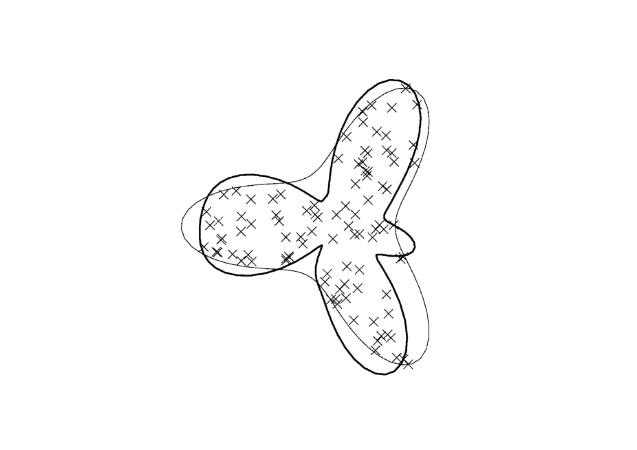
Figure 2: Worst situation. Thin line: $f$, bold line: $\hat{f}^{\mathrm{pol}}_{n}$.

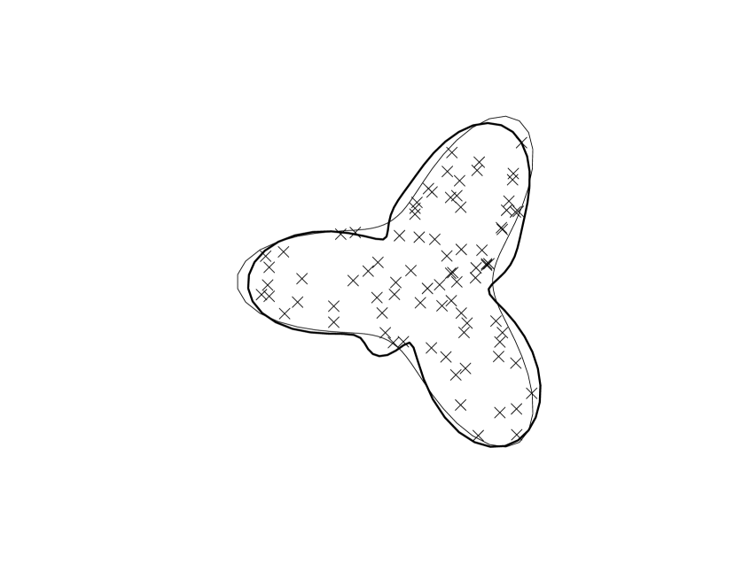
Figure 3: Best situation. Thin line: $f$, bold line: $\hat{f}^{\mathrm{pol}}_{n}$.

– Finally, the best situation (i.e. the estimation corresponding to the smallest $L_{1}$ error) is represented on Figure 3 and the worst situation (i.e. the estimation corresponding to the largest $L_{1}$ error) is represented on Figure 2.

The results are visually satisfying. More precisely, denoting by $\xi_{n}$ the relative $L_{1}-$ error defined by

$$\xi_{n}=\frac{\int_{0}^{2\pi}|\hat{f}_{n}^{\mathrm{pol}}(x)-f(x)|dx}{\int_{0}^{2\pi}f(x)dx},$$

the maximum observed value of $\xi_{n}$ is $9.6\%$ (corresponding to Figure 2), the minimum observed value is $3.8\%$ (corresponding to Figure 3) and the mean value is $6.2\%$.

5 Proofs

5.1 Proofs of section 3

The proofs of Theorem 1 and Theorem 2 follow the same lines. They are based on results of Menneteau (2007) for homogeneous processes and on an approximation argument.

1. First, we show in Lemma 1 that one can associate to $N_{n}$ a homogeneous process thanks to a convenient transformation. More precisely, let $(\Pi_{n})_{n\geq 1}$ denote the sequence of counting processes defined by

$$\Pi_{n}:D\in\mathcal{E}\otimes\mathcal{B}\left(\mathbb{R}\right)\mapsto\#\left\{\left(X_{n,i},\Phi_{X_{n,i}}\left(Y_{n,i}\right)\right)\in D\right\}.$$

Lemma 1

Suppose ($\Phi$) holds. Then, in situation (P) (resp. (E)), $\Pi_{n}$ is associated with a Poisson (resp. an empirical) process on $E\times\mathbb{R}^{+},$ with mean measure $nc\;\mathbf{1}_{G}\left(x,v\right)\;\nu(dx)\;dv\,,$ where

$$G=\{(x,v):x\in E\;;\;0\leq v\leq~{}g(x)\}.$$ (13)

Proof. In situation (P), the result follows from the Mapping Theorem (see Kingman (1993), p. 18). In situation (E), the result is obtained by a simple change of variable (see Cohn (1980), Theorem 6.1.6).   

2. As previously remarked in section 2, asymptotic results were already established for homogeneous processes. For convenience of notation, we write $\hat{c}_{1,n}(x)=\hat{c}_{n}$ and $\hat{f}_{n}(x)=\hat{f}_{n}(x;\hat{c}_{n})$. Following (4), we define for $x\in E$ :

$$\hat{g}_{n}(x)=\hat{g}_{n}\left(x;\hat{c}_{n}\right)=\Phi_{x}(\hat{f}_{n}(x))=\sum_{r=1}^{k_{n}}\nu_{n,r}\kappa_{n,r}(x)\left(\Phi_{X_{n,r}^{*}}(Y_{n,r}^{\ast})+\frac{1}{n\hat{c}_{n}(x)\nu_{n,r}}\right)$$

an estimator of $g(x)$, the frontier of the homogeneous process. Therefore, one can apply to $\hat{g}_{n}$ the following results, proved in Menneteau (2007), which assert that Theorem 1 and Theorem 2 hold with $\varphi=1$.

Proposition 1

i) Let $\varepsilon_{n}=1$ and suppose $(\Phi)$, $\left(\mathrm{H.1}\right)$-$\left(\mathrm{H.6}\right)$ are verified. Let $\hat{c}_{1,n}$ and $\hat{c}_{2,n}$ verifying respectively $(\mathrm{C.1})$ and $(\mathrm{C.2})$. Then, for all $\left(x_{1},...,x_{p}\right)\subset E,$

$$\left\{\frac{n\hat{c}_{2,n}(x_{j})}{\kappa_{n}\left(x_{j}\right)}\left(\hat{g}_{n}\left(x_{j};\hat{c}_{1,n}\right)-g\left(x_{j}\right)\right):1\leq j\leq p\right\}\underset{\mathcal{D}}{\rightarrow}N\left(0,\Sigma_{\left(x_{1},...,x_{p}\right)}\right).$$

ii) Let $\varepsilon_{n}\downarrow 0$ and suppose $(\Phi)$, $\left(\mathrm{H.1}\right)$-$\left(\mathrm{H.6}\right)$ are verified. Let $\hat{c}_{1,n}$ and $\hat{c}_{2,n}$ verifying respectively $(\mathrm{C.1})$ and $(\mathrm{C.2})$. For all $\left(x_{1},...,x_{p}\right)\subset E$ such that $\Sigma_{\left(x_{1},...,x_{p}\right)}$ is regular, the sequence of random vectors

$$\left\{\frac{\varepsilon_{n}^{1/2}n\hat{c}_{2,n}(x_{j})}{\kappa_{n}\left(x_{j}\right)}\left(\hat{g}_{n}\left(x_{j};\hat{c}_{1,n}\right)-g\left(x_{j}\right)\right):1\leq j\leq p\right\}$$

follows the large deviations principle in $\mathbb{R}^{p}$ with speed $(\varepsilon_{n})$ and good rate function $I$.

3. We now derive the asymptotic behavior of $\hat{f}_{n}$ from that of $\hat{g}_{n}$ by an approximation argument given in the next lemma.

Lemma 2

If $\left(\mathrm{H.1}\right)$-$\left(\mathrm{H.7}\right)$ hold and $\hat{c}_{n}$ verifies $(\mathrm{C.1})$, then

$$\mathop{\lim\sup}_{n\to\infty}\varepsilon_{n}\log P\left(\varepsilon_{n}^{1/2}\frac{nc}{\kappa_{n}(x)}\left|\varphi(x,f(x))(\hat{f}_{n}(x;\hat{c}_{n})-f(x))-(\hat{g}_{n}(x;\hat{c}_{n})-g(x))\right|\geq\eta\right)=-\infty.$$ (14)

Proof. The result is straightforward if $\varphi$ is a constant function. We thus focus on the case where, by (H.7),

$$\varepsilon_{n}^{-1/2}\kappa_{n}(x)/n\to 0$$ (15)

as $n\to\infty$. For all $x\in E$, there exists $h_{n}(x)\in[\min(g(x),\hat{g}_{n}(x)),\max(g(x),\hat{g}_{n}(x))]$, such that

$$\hat{f}_{n}(x)-f(x) = \Phi_{x}^{-1}(g(x)+(\hat{g}_{n}(x)-g(x)))-\Phi_{x}^{-1}(g(x))$$

$$= (\Phi_{x}^{-1})^{\prime}(g(x))(\hat{g}_{n}(x)-g(x))+\frac{1}{2}(\Phi_{x}^{-1})^{\prime\prime}(h_{n}(x))(\hat{g}_{n}(x)-g(x))^{2}.$$

Remarking that $(\Phi_{x}^{-1})^{\prime}(g(x))=1/\varphi(x,f(x))$, we obtain that

$$\varphi(x,f(x))(\hat{f}_{n}(x)-f(x))=(\hat{g}_{n}(x)-g(x))+\frac{1}{2}\varphi(x,f(x))(\Phi_{x}^{-1})^{\prime\prime}(h_{n}(x))(\hat{g}_{n}(x)-g(x))^{2}.$$ (16)

Set $\eta>0$ and for all $\alpha>0$ introduce

$$I_{n}(x,\alpha,\varphi) = \left]g(x)-\alpha\frac{\kappa_{n}(x)}{nc\varepsilon_{n}^{1/2}},g(x)+\alpha\frac{\kappa_{n}(x)}{nc\varepsilon_{n}^{1/2}}\right[,$$

$$M_{n}(x,\alpha,\varphi) = \sup_{u\in I_{n}(x,\alpha,\varphi)}\left|(\Phi_{x}^{-1})^{\prime\prime}(u)\right|$$

$$= \sup_{u\in I_{n}(x,\alpha,\varphi)}\frac{\left|\partial\varphi(x,\Phi_{x}^{-1}(u))/\partial y\right|}{\varphi^{3}(x,\Phi_{x}^{-1}(u))}.$$

From (16), and since $|h_{n}(x)-g(x)|\leq|\hat{g}_{n}(x)-g(x)|$, it follows that

$$\varepsilon_{n}^{1/2}\frac{nc}{\kappa_{n}(x)}\left|\varphi(x,f(x))(\hat{f}_{n}(x)-f(x))-(\hat{g}_{n}(x)-g(x))\right|1_{\{\frac{nc\varepsilon_{n}^{1/2}}{\kappa_{n}(x)}|\hat{g}_{n}(x)-g(x)|<\alpha\}}$$

$$\leq \frac{\kappa_{n}(x)}{2nc\varepsilon_{n}^{1/2}}\varphi(x,f(x))M_{n}(x,\alpha,\varphi)\left(\frac{nc\varepsilon_{n}^{1/2}}{\kappa_{n}(x)}|\hat{g}_{n}(x)-g(x)|\right)^{2}1_{\{\frac{nc\varepsilon_{n}^{1/2}}{\kappa_{n}(x)}|\hat{g}_{n}(x)-g(x)|<\alpha\}}$$

$$\leq \frac{\kappa_{n}(x)}{2nc\varepsilon_{n}^{1/2}}\varphi(x,f(x))M_{n}(x,\alpha,\varphi)\alpha^{2}$$

$$< \eta,$$

eventually, since from (15), $I_{n}(x,\alpha,\varphi)\to\{g(x)\}$ as $n\to\infty$ and thus

$$M_{n}(x,\alpha,\varphi)\to\frac{\left|\partial\varphi(x,f(x))/\partial y\right|}{\varphi^{3}(x,f(x))}.$$

Consequently, for all large $\alpha$

$$\mathop{\lim\sup}_{n\to\infty}\varepsilon_{n}\log P\left(\varepsilon_{n}^{1/2}\frac{nc}{\kappa_{n}(x)}\left|\varphi(x,f(x))(\hat{f}_{n}(x)-f(x))-(\hat{g}_{n}(x)-g(x))\right|\geq\eta\right)$$

$$\leq \mathop{\lim\sup}_{n\to\infty}\varepsilon_{n}\log P\left(\frac{nc\varepsilon_{n}^{1/2}}{\kappa_{n}(x)}|\hat{g}_{n}(x)-g(x)|\geq\alpha\right)$$

$$\leq -\frac{\alpha^{2}}{2\sigma^{2}(x)}$$

where $\sigma^{2}(x)=\sigma(x,x)$ with Proposition 1. Letting $\alpha\to\infty$ gives the result.   

4. The proofs of the announced results are now straightforward:

Proofs of Theorem 1 and Theorem 2: a) First, we prove the theorems for $\hat{c}_{2,n}(x)=c$. By Lemma 1, we can apply Proposition 1 to obtain the expected weak convergence and moderate deviations principle for $(\hat{g}_{n}(x)-g(x))$. From Lemma 2, $(\hat{g}_{n}(x)-g(x))$ and $\varphi(x,f(x))(\hat{f}_{n}(x)-f(x))$ share the same asymptotic behavior in terms of weak convergence and moderate deviations principles.
b) In the general case, it is sufficient to prove that

$$\mathop{\lim\sup}_{n\to\infty}\varepsilon_{n}\log P\left(\varepsilon_{n}^{1/2}\frac{n}{\kappa_{n}(x)}\left|\hat{c}_{n,2}(x)-c\right|\left|\hat{f}_{n}(x)-f(x)\right|\geq\eta\right)=-\infty.$$ (17)

To this aim, observe that, for all large $\alpha>0$,

$$P\left(\varepsilon_{n}^{1/2}\frac{n}{\kappa_{n}(x)}\left|\hat{c}_{n,2}(x)-c\right|\left|\hat{f}_{n}(x)-f(x)\right|\geq\eta\right)$$

$$\leq P\left(\left|\hat{c}_{n,2}(x)-c\right|\geq c/\alpha\right)$$

$$+ P\left(\varepsilon_{n}^{1/2}\frac{nc}{\kappa_{n}(x)}\left|\hat{f}_{n}(x)-f(x)\right|\geq\eta\alpha\right).$$

Thus, from (C.2) and the part a) of the proof,

$$\mathop{\lim\sup}_{n\to\infty}\varepsilon_{n}\log P\left(\varepsilon_{n}^{1/2}\frac{n}{\kappa_{n}(x)}\left|\hat{c}_{n,2}(x)-c\right|\left|\hat{f}_{n}(x)-f(x)\right|\geq\eta\right)$$

$$\leq \mathop{\lim\sup}_{n\to\infty}\varepsilon_{n}\log P\left(\varepsilon_{n}^{1/2}\frac{nc}{\kappa_{n}(x)}\left|\hat{f}_{n}(x)-f(x)\right|\geq\eta\alpha\right)$$

$$\leq -\frac{\alpha^{2}\eta^{2}}{2\sigma^{2}(x)}.$$

Letting $\alpha\to\infty$ gives the intended result (17).   

Proof of Corollary 1 and Corollary 2: Mimicking the part b) of the proof of Theorem 1 and Theorem 2, it is sufficient to prove that

$$\mathop{\lim\sup}_{n\to\infty}\varepsilon_{n}\log P\left(\left|\varphi(x,\hat{f}_{n}(x))-\varphi(x,f(x))\right|\geq\eta\right)=-\infty.$$ (18)

Since, from ($\Phi$), $\varphi$ is continuous at point $f(x)$, there exists $\delta>0$ such that

$$|y-f(x)|<\delta\Rightarrow|\varphi(x,f(x))-\varphi(x,\hat{f}_{n}(x))|<\eta.$$

Hence, for all large $\alpha>0$,

$$\mathop{\lim\sup}_{n\to\infty}\varepsilon_{n}\log P\left(\left|\varphi(x,\hat{f}_{n}(x))-\varphi(x,f(x))\right|\geq\eta\right)$$

$$\leq \mathop{\lim\sup}_{n\to\infty}\varepsilon_{n}\log P\left(\varepsilon_{n}^{1/2}\frac{nc}{\kappa_{n}(x)}\left|\hat{f}_{n}(x)-f(x)\right|\geq\delta\varepsilon_{n}^{1/2}\frac{nc}{\kappa_{n}(x)}\right)$$

$$\leq \mathop{\lim\sup}_{n\to\infty}\varepsilon_{n}\log P\left(\varepsilon_{n}^{1/2}\frac{nc}{\kappa_{n}(x)}\left|\hat{f}_{n}(x)-f(x)\right|\geq\alpha\right)$$

$$\leq -\frac{\alpha^{2}}{2\sigma^{2}(x)}.$$

Letting $\alpha\to\infty$ gives the intended result (18).   

5.2 Proofs of section 4

Proofs of Theorem 3 and Theorem 4 both rely on the following lemma which permits to apply Theorem 1 and Theorem 2.

Lemma 3

In situation (P) (resp. (E)), $\left(X_{n,i},Y_{n,i}\right)_{i\geq 1}$ is a Poisson (resp. an empirical) process with mean measure $n\;c\;\gamma_{d}\;y^{d-1}\;\mathbf{1}_{S}\left(x,y\right)\;h_{d}(x)\;dx\;dy$.

Proof. Note that the Jacobian of the inverse polar transformation $P_{d}^{-1}$ is

$$J(x,y)=y^{d-1}\prod_{j=1}^{d-1}(\sin x_{j})^{d-1-j}=\gamma_{d}\;y^{d-1}\;h_{d}(x).$$

Hence, in situation (P), the result follows from the Mapping Theorem (see Kingman (1993), p. 18). In situation (E), the result is obtained by a change of variable (see Cohn (1980), Theorem 6.1.6).   

Lemma 4

With (5), (7) and (8), estimator (3) can be rewritten as

$$\hat{f}_{n}^{\mathrm{pol}}(x)=\left(\sum_{r=1}^{k_{n}}\left(\int_{I_{n,r}}K_{n}(x,t)\nu(dt)+\frac{\int_{E}K_{n}(x,t)\nu(dt)}{k_{n}N_{n,r}}\right)\left(Y_{n,r}^{\ast}\right)^{d}\right)^{1/d}.$$

Proof. From (3) and (5),

$$\hat{f}_{n}^{\mathrm{pol}}(x)=\left(\overset{k_{n}}{\underset{r=1}{\sum}}\kappa_{n,r}(x)\left(\nu_{n,r}\left(Y_{n,r}^{\ast}\right)^{d}+\frac{d}{\gamma_{d}}\frac{1}{n\hat{c}_{n}}\right)\right)^{1/d}.$$

Thus, taking account of (7) and (8),

$$\hat{f}_{n}^{\mathrm{pol}}(x) = \left(\sum_{r=1}^{k_{n}}\int_{I_{n,r}}K_{n}(x,t)\nu(dt)\left(\left(Y_{n,r}^{\ast}\right)^{d}+\frac{1}{k_{n}}\sum_{s=1}^{k_{n}}\frac{\left(Y_{n,s}^{\ast}\right)^{d}}{N_{n,s}}\right)\right)^{1/d}$$

$$= \left(\sum_{r=1}^{k_{n}}\left(\int_{I_{n,r}}K_{n}(x,t)\nu(dt)+\frac{\int_{E}K_{n}(x,t)\nu(dt)}{k_{n}N_{n,r}}\right)\left(Y_{n,r}^{\ast}\right)^{d}\right)^{1/d}.$$

 

Proof of Theorem 3 and Theorem 4: First, Lemma 4.5 in Menneteau (2007) shows that, under (H.1) and (H.2), conditions (C.1) and (C.2) hold for $\hat{c}_{n}$ defined in (8). Second, in the proofs of Theorem 3.1 and Theorem 3.2 in Menneteau (2007), it is shown that conditions (H.1), (H.2), (K.1)-(K.6) imply conditions (H.1)-(H.6) of Theorem 1 and Theorem 2 and that $\kappa_{n}(x)=k_{n}^{1/2}\|K_{n}(x,.)\|_{2}(1+o(1))$. Thus, (K.7) implies (H.7).   

Proof of Corollary 3: From Menneteau (2007), Corollary 3.8, (i)–(v) imply (H.1), (H.2) and (K.1)-(K.6). Moreover it is clear that (i), (ii) give (K.7) since, by Tolstov (1976), $\|K_{n}^{D}(x,.)\|_{2}=(\ell_{n}+1)^{1/2}$.   

References

Baillo, A. and Cuevas, A. (2001) On the estimation of a star-shaped set. Adv. Appl. Proba., 33(4), 717–726.

Chevalier J. (1976) Estimation du support et du contour d’une loi de probabilité Ann. Inst. H. Poincaré, sect. B, 12, 4, 339–364.

Cohn, D. (1980) Measure theory. Birkhäuser.

Dembo, A. and Zeitouni, O. (1993) Large Deviations Techniques and Applications. Jones and Bartlett, Boston and London.

Deprins, D., Simar, L. and Tulkens, H. (1984) Measuring Labor Efficiency in Post Offices. in The Performance of Public Enterprises: Concepts and Measurements by M. Marchand, P. Pestieau and H. Tulkens, North Holland ed, Amsterdam.

Devroye, L.P. and Wise, G.L. (1980) Detection of abnormal behavior via non parametric estimation of the support. SIAM J. Applied Math., 38, 448–480.

Geffroy, J. (1964) Sur un problème d’estimation géométrique. Publications de l’Institut de Statistique de l’Université de Paris, XIII, 191–200.

Gensbittel, M.H., (1979) Contribution à l’étude statistique de répartitions ponctuelles aléatoires. PhD Thesis, Université Pierre et Marie Curie, Paris.

Girard, S. and Menneteau, L. (2005) Central limit theorems for smoothed extreme value estimates of Poisson point processes boundaries. Journal of Statistical Planning and Inference, 135, 433–460.

Hall, P., Park, B. U. and Stern, S. E. (1998) On polynomial estimators of frontiers and boundaries. J. Multiv. Analysis, 66, 71–98.

Hardy A. and Rasson J. P. (1982) Une nouvelle approche des problèmes de classification automatique. Statistique et Analyse des données, 7, 41–56.

Kallenberg, W. (1983a) Intermediate efficiency, theory and examples. Annals of Statistics, 11, 170–182.

Kallenberg, W. (1983b) On moderate deviation theory in estimation. Annals of Statistics, 11, 498–504.

Kingman, J. (1993) Poisson processes. Oxford Studies in Probability, 3, Oxford: Clarendon Press.

Korostelev, A. P. and Tsybakov, A. B. (1993) Minimax theory of image reconstruction. Lecture Notes in Statistics, 82, Springer Verlag, New-York.

Mardia, K., Kent, J. and Bibby, J. (1979) Multivariate analysis. Academic Press London.

Menneteau, L. (2007) Multidimensional limit theorems for smoothed extreme value estimates of point process boundaries. ESAIM: Probability and Statistics, to appear.

Renyi, A. and Sulanke, R. (1963) Uber die konvexe Hülle von n zufälligen gewählten Punkten. Z. Wahrscheinlichkeitstheorie verw. Geb. 2, 75–84.

Stone, C. (1982) Optimal global rates of convergence for nonparametric regression, Annals of Statistics, 10, 1040–1053.

Tolstov, G.P. (1976) Fourier Series. 2nd ed., Dover Publications, New York.

⁽¹⁾ Team MISTIS, INRIA Rhône-Alpes, ZIRST, 655 avenue de l’Europe,
38330 Montbonnot, France, Stephane.Girard@inrialpes.fr ⁽²⁾ EPS/I3M, Université Montpellier 2, place Eugène Bataillon,
34095 Montpellier cedex 5, France, mennet@math.univ-montp2.fr

Figure 1: Two different parametrizations of the point process support. Left: $S^{\mathrm{pol}}$ is described with polar coordinates, right: $S$ is described in Cartesian coordinates.