Experimental Design for the Gemini Planet Imager

Abstract

The Gemini Planet Imager (GPI) is a high performance adaptive optics system being designed and built for the Gemini Observatory. GPI is optimized for high contrast imaging, combining precise and accurate wavefront control, diffraction suppression, and a speckle-suppressing science camera with integral field and polarimetry capabilities. The primary science goal for GPI is the direct detection and characterization of young, Jovian-mass exoplanets. For plausible assumptions about the distribution of gas giant properties at large semi-major axes, GPI will be capable of detecting more than 10% of gas giants more massive than 0.5 $M_{J}$ around stars younger than 100 Myr and nearer than 75 parsecs. For systems younger than 1 Gyr, gas giants more massive than 8 $M_{J}$ and with semi-major axes greater than 15 AU are detected with completeness greater than 50%. A survey targeting young stars in the solar neighborhood will help determine the formation mechanism of gas giant planets by studying them at ages where planet brightness depends upon formation mechanism. Such a survey will also be sensitive to planets at semi-major axes comparable to the gas giants in our own solar system. In the simple, and idealized, situation in which planets formed by either the “hot-start” model of Burrows et al. (2003) or the core accretion model of Marley et al. (2007), a few tens of detected planets are sufficient to distinguish how planets form.

1. Introduction

The past decade has seen extraordinary progress in detection of exoplanets with the deployment of custom designed systems that use the Doppler method, such as HARPS (Mayor et al., 2003), and the transit method, such as Kepler (Borucki et al., 2003). Exoplanetary systems are also being discovered using microlensing (Gould et al., 2010; Sumi et al., 2010). No planets are confirmed to have been detected using astrometry, though there are disputed claims of some detections, including a companion to VB 10 (Pravdo & Shaklan, 2009; Bean et al., 2010; Anglada-Escudé et al., 2010). Even so, the upcoming Gaia mission is expected to have astrometric precision of $\sim 8\mu$as, and thus be able to astrometrically discover the hundreds of exoplanets and exoplanetary systems expected to have astrometric signals $>30\;\mu$as around stars within 200 parsecs (Casertano et al., 2008). Polarimetric detection of HD 189733 b has also been claimed by Berdyugina et al. (2008), but Wiktorowicz (2009) was unable to reproduce the detection.

These methods are indirect, and provide different information about the planets that they detect. From radial velocity surveys alone, the period, eccentricity and a minimum mass may be measured for detected planets. For planets that also transit their hosts, it is possible to learn the inclination of the orbit and planet radius, given simple assumptions about the system and knowledge of the stellar mass-radius relation, which then give the mass and density of the planet (Seager & Mallén-Ornelas, 2003). Mid-IR exoplanetary light has been detected in secondary eclipses by Spitzer (Charbonneau et al., 2005; Grillmair et al., 2007; Richardson et al., 2007; Fressin et al., 2010; O’Donovan et al., 2010), though information about the planet spectrum itself is limited by the photon shot noise of the primary.

Marcy et al. (2008) lists 228 extrasolar planets, with 5% of targeted stars possessing massive planets, and shows that a diversity of exoplanet systems exists. Though the number of radial velocity confirmed planets has nearly doubled since, and many more planet candidates exist in the first four months of Kepler data (Borucki et al., 2011), radial velocity and transit surveys leave several long-standing questions about planetary systems unanswered. How do planets form? Is the solar system typical? What is the abundance of solar-like systems? These surveys also raise new questions, including what produces the dynamical diversity in exoplanetary systems?

The prospects for indirect planet detection techniques alone to answer these questions is limited. With the exception of microlensing, the effectiveness of these techniques at detecting exoplanets decreases at large semi-major axes. For a reliable detection with radial velocity, a significant fraction of an orbital period must elapse. As such, radial velocity surveys are only now reaching the precision and lifetime necessary to detect Jupiter, and thus do not yet constrain the frequency of solar system analogs. For example, in the Keck radial velocity search that began in 1996 July (Butler et al., 2006), only planets with $a\leq 6$ AU have completed one orbit. The median semi-major axis of known exoplanet orbits is approximately 1 AU, and HD 190984 b is the only planet with with $a>6$ AU (Santos et al., 2010). As the time baseline of surveys grows, the semi-major axes probed increase according to $a=P^{2/3}$, meaning improving the statistics at large semi-major axes will be challenging. Doppler surveys have also been focused on a small range of stellar masses and ages, as precise radial velocity measurement requires strong stellar spectral features and low activity. This has limited studies of exoplanet trends with stellar properties beyond basic correlations between host star mass and metallicity and the probability of hosting a planet within a few AU (Johnson et al., 2010).

Direct imaging constitutes the next step in characterizing other planetary systems. Many previous attempts to directly image substellar companions to stars have already placed stringent constraints on the presence of giant planets on wide orbits (Schroeder et al., 2000; Masciadri et al., 2005; Kasper et al., 2007; Biller et al., 2007; Lafrenière et al., 2007b; Apai et al., 2008; Heinze et al., 2010; Leconte et al., 2010). There are also projects already underway, such as NICI (Liu et al., 2010) and SEEDS (Tamura, 2009), or that are near deploying, such as SPHERE (Beuzit et al., 2010) and GPI. Thus far, planet detections through direct imaging have been limited by difficulty in achieving high contrast at small angular separations, but instruments are now reaching the threshold at which planet detection by direct imaging is promising. Direct imaging is highly complementary to Doppler surveys. Unlike Doppler searches, direct imaging is sensitive at large semi-major axes, as planets can be found without waiting for an orbit to complete—a condition that renders Doppler detection of planets on Neptune-like orbits with semi-major axes of 30 AU and periods of 160 yr impractical. Fourier decomposition, which underlies Doppler and astrometric detection, is also subject to aliasing and beat phenomena, and suffers confusion when multiple planets are present. A direct search that can probe beyond 5 AU will thus bring statistical significance to these studies.

The goal of direct detection is to spatially separate the exoplanet light from that of its primary. This affords access to exoplanet atmospheres, which yields fundamental information including effective temperature, gravity, atmospheric composition and abundances, orbital motion, and perhaps even weather and planetary spin (via polarization associated with rotation-induced oblateness; Marley 2010). Direct imaging may also reveal the role of giant impacts, though 10 to 100 planets $\sim$ 10 Myr old may need to be discovered in order to expect to find a single gas giant post impact (Anic et al., 2007), or lead to discovery of time dependent atmospheric phenomena.

Most importantly, by probing large semi-major axes, direct imaging will see gas giants beyond the “snow line,” which is where they are expected to form, and extend out to the greatest distances at which giant planets can form. The location of the region of interest depends on at least two competing factors: time-scales for planet building and the availability of raw material. Dynamical and viscous time scales in the disk are shorter at small radii, while for typical surface-density laws the amount of mass increases with radius, with a jump in the abundance of solid material beyond the “snow line” where ices condense. This change in the surface density of solid material occurs at 2.7 AU in the Hayashi model (Hayashi, 1981). The location of this boundary depends on the disk structure (Sasselov & Lecar, 2000), but for solar type stars, the zone of interest is beyond that which is readily probed by the Doppler method. The discovery of giant planets far beyond the snow line would tend to favor theories of planet formation by gravitational instability over solid core condensation and accretion. At larger orbital radii ($>$ 20–30 AU), gas-cooling times become shorter than the Keplerian shearing time (e.g., Kratter et al. 2010)—a necessary condition for runaway gravitational instability (Gammie, 2001; Johnson & Gammie, 2003; Boss, 2002)—while solid core growth by collisional coagulation of planetesimals proceeds prohibitively slowly (Goldreich et al., 2004). Even so, new ideas about coupling between migration and core accretion suggest significantly increased growth, allowing the formation of planets well beyond the snow line (Levison et al., 2010). The structure of our own solar system implies that a full picture of planet formation cannot be constructed without reaching out to 30 or 40 AU. Millimeter observations of T Tauri disks support this, as typical disk radii fall in the range 50–100 AU (Isella et al., 2009).

The initial conditions, composition, and equation of state all influence evolution of young gas giant planets. Gas giants will take tens to hundreds of millions of years to “forget” their post-formation entropy, meaning temperatures and luminosities of young planets will reveal their past (Marley et al., 2007). Stellar properties, in particular mass and metallicity, will also influence planet formation. The observed planet-metallicity correlation in Doppler planets has been interpreted as supporting core accretion as the formation mechanism of gas giants (Fischer & Valenti, 2005; Johnson et al., 2010). Metal-rich disks are expected to have longer lifetimes (Ercolano & Clarke, 2010) and enhanced clump formation (Johansen et al., 2009), all increasing the likelihood of planet formation for those formed by core accretion. Formation by disk instability is not expected to be sensitive to stellar metallicity (Boss, 2002). This has led to the suggestion that low metallicity stars will preferentially form planets by disk instability on wide orbits, while high metallicity stars will host planets on short period orbits formed by core accretion (Boley, 2009; Dodson-Robinson et al., 2009). Stellar metallicity is also expected to influence planet appearance. Planets formed via core accretion are predicted to themselves have super-stellar metallicity (Pollack et al., 1996; Fortney et al., 2008). Though gas giants more massive than $\sim 5M_{J}$ formed by disk instability may also have super-stellar atmospheric metallicities, less massive gas giants should have metal depleted atmospheres (Helled & Schubert, 2008). Exoplanet infrared colors are predicted to be sensitive to atmospheric metal abundances, so direct imaging and spectroscopy will reveal information about a planet’s formation (Fortney et al., 2008).

Another reason to image the outer regions of extrasolar systems is to probe them for vestiges of planetary migration. Ninety percent of the Doppler sample consists of massive planets with $a<$ 3 AU, suggesting that they migrated inwards to their present locations. A variety of mechanisms may drive orbital evolution; the tidal gravitational interaction between the planet and a viscous disk (Goldreich & Tremaine, 1980), the gravitational interaction between two or more Jupiter mass planets (Rasio & Ford, 1996), and the interaction between a planet and a planetesimal disk (Murray et al., 1998). It is energetically favorable for a Keplerian disk to evolve by transporting mass inward and angular momentum outward (Lynden-Bell & Pringle, 1974). Consequently, inward planetary drift appears inevitable, and this is what is found in certain simulations (Trilling et al., 2002; Armitage et al., 2002; Matsuyama et al., 2003). However, if planets form while the disk is being dispersed, or if multiple planets are present, outward migration can also occur. In a system consisting initially of two Jupiter-like planets, a dynamical instability may eject one planet while the other is left in a tight, eccentric orbit. The second planet is not always lost; the observed Doppler exoplanet eccentricity distribution can be reproduced if the 51 Pegasi systems are formed by planet-planet scattering events and the second planet typically remains bound in a wide ($a>$ 20 AU), eccentric orbit (Rasio & Ford, 1996; Marzari & Weidenschilling, 2002; Veras et al., 2009). Divergent migration of pairs of Jupiter-mass planets within viscous disks leads to mutual resonance crossings and excitation of orbital eccentricities such that the resultant ellipticities are inversely correlated with planet masses (Chiang et al., 2002). Given decreasing disk viscosity with radius and the consequent reduction in planetary mobility with radius, we expect eccentricities to decrease with radius, perhaps sharply if the magneto-rotational instability is invoked (Sano et al., 2000). By contrast, excitation of eccentricity by disk-planet interactions requires no additional planet to explain the ellipticities of currently known solitary planets (Goldreich & Sari, 2003). Clearly, observations of the incidence, mass, and eccentricity distributions of multiple planet systems would sharpen ideas regarding how planetary orbits are sculpted.

There have already been a number of planets and planet candidates discovered by direct imaging, including beta Pic b (8 AU/8 $M_{J}$; Lagrange et al. 2009), the upper Sco object 1RXS J160929.1-210524 (330 AU/8 $M_{J}$ Lafrenière et al. 2008), HR 8799 b, c, d, and e (24, 38, 68, and 14 AU/10, 10, 7, and 10 $M_{J}$; Marois et al. 2008a, 2010b), and Fomalhaut b (120 AU/$<$ 2 $M_{J}$ Kalas et al. 2008). While the sample of exoplanets is incomplete for $a>$ 5 AU, indirect searches continue to hint that the semi-major axis distribution is at least flat, and possibly rising, in $dN/d\log(a)$ beyond 5 AU (Cumming et al., 2008). The sample of six microlensed planets beyond the ice line supports this trend (Sumi et al., 2010; Gould et al., 2010). Thus, a direct imaging search of outer solar system regions (5–50 AU), such as proposed here, would increase the total number of planets found relative to those in inner solar system orbits ($<5$ AU). The goal of direct imaging is to assemble the first statistically significant sample of exoplanets that probes beyond the reach of indirect searches and quantifies the abundance of solar systems like our own.

2. Overview of the GPI instrument

The Gemini Planet Imager is configured to allow high contrast ($>10^{7}$) imaging on angular scales of the diffraction limit ($\sim 5-20\lambda/D$). High-contrast imaging with current AO systems is almost completely limited by quasi-static artifacts caused by slowly evolving wavefront errors. These originate from many sources, including inadequately calibrated non-common-path errors that arise from the difference between the science and wavefront sensing paths, uncorrectable high spatial frequency errors on instrumental and telescope optics, aliased high-frequency wavefront errors (Poyneer & Macintosh, 2004), chromatic errors, reflectivity variations, and Fresnel propagation effects. Although these can be partially attenuated through techniques like angular differential imaging (Marois et al., 2006), the errors evolve rapidly enough that ADI-like techniques do not operate well at small angles where it takes significant time for enough field rotation to accumulate. Unfortunately, these small angles are also the scales that correspond to our own solar system for most nearby young stars. GPI was designed from the beginning to minimize these quasi-static error sources and hence allow high-contrast imaging approaching the photon noise limit. For more detail, see Macintosh et al. (2006, 2008).

The GPI system consists of five key subsystems: an AO system, a coronagraph, an interferometer, an integral field spectrograph, and a software system.

The AO system makes fast measurements of the instantaneous wavefront and provides wavefront control via a tip-tilt stage and two deformable mirrors, one conventional piezoelectric and one high-order silicon micro-electro-mechanical-system (MEMS) device. The high-order AO system has 43 actuators across the diameter of the 7.8-m Gemini South primary mirror and operates at at an update rate of 1.5 kHz. The AO system uses a spatially-filtered Shack-Hartmann wavefront sensor to minimize aliasing and have uniform response in varying atmospheric seeing (Poyneer & Macintosh, 2004). The anti-aliasing produces a characteristic square “dark hole” region, $\sim 43\lambda/D$ on a side.

The coronagraph is an apodizer-pupil Lyot coronagraph (APLC), and it controls diffraction (Soummer et al., 2006). This combines a carefully-designed input apodization with a focal-plane occulting stop (in GPI, a mirror with a central hole) and a Lyot pupil stop matched to the input telescope pupil size. The GPI APLC implementation is optimized for achromatic performance to improve multi-wavelength speckle suppression. Each waveband has a hard-edged occulter hole with a radius of 2.8 $\lambda/D$, but that hole is also surrounded by a bright Airy ring, so high contrast is only fully practical at ($\sim 4$–$5\lambda/D$).

The interferometer provides low-temporal bandwidth precise and accurate measurements at the science wavelength of the time-averaged wavefront delivered to the coronagraph occulting spot. This information is used to remove slowly-evolving quasi-static errors due to flexure and changes in the response of the main visible-light wavefront sensor.

The science instrument is an integral field spectrograph (IFS) that images in simultaneous multiple wavelength channels. The lenslet-based IFS has sampling of 0.014$\arcsec$ per lenslet, with a square field of view of 2.8$\arcsec$ on a side. Each spatial pixel is dispersed into a spectrum with resolution $R\sim 45$. A single observation covers one of the $Y$, $J$, or $H$ bands, or half of the $K$ band, which is split in to $K_{1}$ and $K_{2}$. Raw detector images are reassembled by a data pipeline into $200\times 200\times 16$ element data cubes. The IFS also includes a differential polarimetry mode, intended for characterization of circumstellar dust and not discussed in this paper. Finally, the software system coordinates communication between the other subsystems and the observatory software.

GPI operates at a Cassegrain focus on the alt/az mount of the Gemini telescope in a fixed orientation with respect to the telescope, to increase instrumental stability and enable ADI post-processing. A typical science observation will consist of an hour long sequence of 30-60 second exposures. This is long enough that read noise and dark current are unimportant contributors to the noise budget, and short enough that image motion during the exposure is minimal.

3. Instrumental Noise Calculations

3.1. Simulations

High-contrast imaging noise can be broken down into two main categories: speckle noise and photon noise. Instantaneous monochromatic high-contrast images consist of a pattern of bright “speckles” surrounding the central core. These speckles have a size of $\sim\lambda/D$, comparable to the image of a planet, and their random fluctuations are usually the main limitation in planet detection in existing high-contrast imaging instruments. In many cases (e.g. atmospheric turbulence wavefront errors), the speckle pattern will evolve rapidly, and after some characteristic speckle lifetime has elapsed the speckle noise will scale with exposure time as $t^{0.5}$ and in a long exposure produce a more uniform halo of light. In addition, any light present in the focal plane due to wavefront errors, whether speckled or uniform, will contribute Poisson photon noise.

In the GPI architecture, we consider the following sources of wavefront error and their corresponding speckle and/or photon noise (Poyneer & Macintosh, 2006; Marois et al., 2008b):

1. Residual atmospheric errors. Even operating at 1.5 kHz, the motion of the turbulent atmosphere will cause changes in wavefront between measurement and the application of a correction. This is the dominant source of mid-to-low frequency wavefront errors. Here, low-frequency errors ($<3$ cycles/pupil) refers to errors at spatial frequencies mostly blocked by the coronagraph occulter, and mid-frequency errors (3–22 cycles/pupil) are those transmitted by the occulter but that are within the controllable range of the deformable mirror. Errors at these frequencies contribute scattered light and photon noise near the star. Higher frequency spatial wavefront errors ($>22$ cycles/pupil) are unsensable and uncorrectable by the GPI AO system and contribute light outside the dark hole. A representative speckle produced by these atmospheric wavefront errors has a lifetime of a few tenths of a second and an amplitude of 60 nm.

2. Wavefront sensor measurement noise. On dimmer stars, the individual wavefront sensor measurements will include a significant noise component that will translate to random errors of position of the deformable mirror. In a Shack-Hartmann wavefront sensor, these errors are not spatially white, but have increasing power at low spatial frequencies. On dim stars, this is again a significant source of scattered light over the whole dark hole region. Speckles associated with this error source randomize at the closed-loop bandwidth of the system, with lifetimes of a few milliseconds, rapidly smoothing out. A typical value is 25 nm for a star with $I=6$ mag.

3. Residual non-common-path wavefront errors. After daytime calibration and closed-loop correction by the precision interferometric wavefront sensor, these are assumed to be $\sim 5$ nm of low-frequency error and $\sim 1$ nm of mid-frequency errors. The amount of light scattered by these small wavefront errors produces a negligible amount of photon noise, but the slowly-varying speckles they produce are a significant source of speckle noise.

4. Reflectivity variations and amplitude errors. The GPI deformable mirrors are operated in phase conjugation mode, correcting the phase errors of the wavefront and producing a symmetric final PSF. As a result, any light scattered by changes in amplitude—for example, from reflectivity variations on the Gemini primary mirror—is uncorrectable. We assign a reflectivity variation to each individual optic in our system (typically 0.1%, rising to 1% for the primary mirror and the MEMS DM, with a $k^{-2.5}$ spatial frequency power spectrum). The light scattered by these reflectivity errors again produces little photon noise but significant speckle noise.

5. Fresnel propagation errors. Surface errors on an optic at an arbitrary location in the GPI optical train will initially produce a pure phase error in the wavefront, but as the wavefront propagates these errors will mix between phase and amplitude (Shaklan & Green, 2006). The finite size of GPI optics will also produce amplitude fluctuations near the edge of the beam. As noted above, GPI will only correct the component of these errors that is realized as phase at the deformable mirrors, not the amplitude component. To mitigate this, GPI optics are located away from focal planes and are of very high quality ($\sim 2$ nm RMS wavefront error typically), but these are still a significant source of persistent and chromatic speckles.

6. Atmospheric scintillation. Classical scintillation causes uncorrectable amplitude fluctuations in the telescope pupil similar to the Talbot propagation errors. Unlike the internal Talbot errors, those from the atmosphere are time varying. Simulations and calculations show that for our typical atmosphere profile this is a negligible contribution to the photon and speckle noise and hence it is ignored.

In addition, normal astronomical noise sources such as sky background, detector readout, and dark current will be present, though for typical GPI targets with $H<8$ mag. these are negligible. Telescope vibrations (windshake or mechanical vibrations of either GPI or the telescope secondary) are not included in this model, in part because the exact vibration environment of the Gemini telescope is unknown. The GPI tilt error budget allocates $<5$ mas RMS to these effects; GPI employs an advanced tip/tilt control algorithm (Poyneer & Véran, 2010) that can cancel out resonant vibrations of the telescope, and the mechanical structure includes tuned-mass damping to cancel internal vibrations. These 5 mas have no significant effect on the coronagraph or on planet detectability.

Modeling all these effects is challenging. Even with simple Fraunhoffer propagation, simulating the AO wavefront correction and propagation to the science focal plane requires several CPU-hours per second of exposure time. Since GPI has been designed to minimize the quasi-static wavefront errors 3, 4, and 5 in the list above, their effects can only be seen after many minutes of integration. As a result, we treat the dynamic and static wavefront errors as independent and treat them in two different simulations. The first simulates the dynamic behavior of the atmosphere and each component of the adaptive optics system to produce short-exposure point spread functions, using Fraunhoffer propagation through the GPI optics and coronagraph. These were run for a standard Gemini Cerro Pachon atmosphere (Tokovinin & Travouillon, 2006) and for stars with brightness ranging from $I$ = 5–9 mag. (Poyneer & Macintosh, 2006). The second, described in Marois et al. (2008b), includes all the quasi-static wavefront error source and full Fresnel propagation through the GPI optical train, but has no atmospheric wavefront errors. Both simulations are run at each IFS wavelength channel within the $H$ band. Photon and speckle noise are evaluated separately in each simulation.

3.2. Post-processing

Speckle noise can be attenuated through post-processing techniques such as ADI. However, this depends critically on the stability of the aberrations producing those speckles. We have assumed no ADI attenuation whatsoever, making the pessimistic assumption that wavefront errors will evolve just fast enough to be unsubtractable over the timescales needed for ADI field rotation. Field rotation will still produce some averaging of the residual speckle noise as the planetary companions move through the speckle noise pattern, so we reduce the speckle noise by an amount equal to the square root of the number of $\lambda/D$ that field rotation will move the planet through in a 1-hour exposure.

Since GPI’s science instrument produces spectral data cubes, speckles can also be attenuated by scaling and subtracting different wavelength channels. We assume post-processing using a simple “double difference” algorithm using three different wavelengths. For the atmospheric speckles, which are almost purely phase errors and hence have well-behaved chromaticity, this attenuates speckle noise by more than 4 to 6 magnitudes at all radii, leaving the atmospheric speckle noise completely negligible. For the quasi-static speckles, especially the Fresnel effects, the speckles are more chromatic and they are attenuated by only 2–3 magnitudes within the dark hole region. Since these speckles are weak to begin with, the residual noise is lower than the photon noise for all but the brightest stars.

This double-difference subtraction will also attenuate the planetary signal, unless the planetary signal contains deep molecular absorption features (e.g. methane), or the wavelength scaling of the speckles cause them to move by more than $2\lambda/D$ through a single spectral band, i.e. at radii greater than $10\lambda/D$ for a 20% bandpass. Although not all planets will show methane absorption, the faintest (and hence most difficult to detect) planets are expected to. The HR 8799 planetary companions do not show methane absorption but are so bright—contrast $\sim 10^{5}$ relative to their F-star host—that they would be easily detected by GPI even without spectral differencing. Hence the use of the spectral-difference contrast curves is appropriate for the Monte Carlo modeling described here. In actual operation, GPI will likely use a more sophisticated approach to PSF subtraction with wavelength and time, likely based on the LOCI algorithm (Lafrenière et al., 2007a) and the SOSIE framework (Marois et al., 2010a). However, this would not significantly change the results here, since in these simulations even with simple spectral differencing GPI is photon-noise rather than speckle-noise limited for stars brighter than $I$ = 6 mag.

3.3. Final instrumental contrast predictions

The results of the instrumental noise calculations are tabulated as a function of stellar brightness and angular separation for each noise source. These tabulated values are used to generate the total number of photons contributed by all sources of noise for some exposure time. A planet may then be considered detectable if the expected number of photons detected from the planet is five times the number of photons contributed by noise. The contrast curves in Figure 1 summarize this result, showing the ratio of five times the overall noise to the number of photons detected from the host star as a function of angular separation. The instrument is expected to reach contrasts better than $10^{-7}$ over an hour long exposure for targets with $I\sim 5$ mag. For brighter targets, the performance remains the same, while the expected contrast declines for dimmer targets. For stars beyond $I\sim$ 10–11 mag., the system performance becomes comparable to existing instruments. For that reason, stars brighter than $I\sim 10$ mag. will make up the majority of GPI targets.

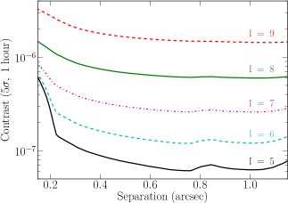
Figure 1.— Contrast curves (5$\sigma$) in the $H$ band as a function of angular separation for five different star $I$ magnitudes, assuming one hour on the target and an A0 star. Photon shot noise dominates for stars with $I>6$ mag., while static speckles dominate for stars with $I<6$ mag. Visit http://planetimager.org for a tabular version of these data.

3.4. Matched filters

Models of the spectral properties of planets (these models will be discussed in more detail in the next section) predict young planets will show many spectral features, rather then being uniformly bright across a wavelength band. For this reason, the integral field spectrograph, which provides 16 spectral channels across each wavelength band, will be important to the success of GPI at detecting planets. A planet may be bright enough in some spectral channels to be above the contrast limit, while its flux when summed over the entire band is not. The model spectrum from Fortney et al. (2008) in Figure 2 is an example of such a case. The flux from this model planet is concentrated in a narrow range of wavelengths, while the rest of the spectral channels contribute primarily noise. When looking at the spectrum, even without the model spectrum to guide the eye, it looks like a clear detection. Yet the overall signal to noise ratio across the entire H band is less than 5, meaning a sum over all spectral channels would yield a non-detection.

Analysis of real data will involve much more than evaluating a planet’s signal to noise ratio and declaring a detection or non-detection. For the purposes of simulating tens of thousands of planets around thousands of stars though, this is a practical approach. Yet the spectral features in planetary atmospheres suggest that generating a planet’s signal to noise ratio by taking a simple sum of all spectral channels will underestimate GPI’s ability to detect that planet. To explore how much the detection rate may be affected, we used model atmospheres to generate matched filters. This was done by degrading the resolution of a model atmosphere at a given surface gravity and temperature to match that of GPI ($\lambda/\Delta\lambda\sim 45$ in the $H$ band), and then weighting each of the spectral channels according to the model predicted flux. These weighted channels are then summed to find the total flux from the planet, and the total noise.

Using matched filters significantly improves survey performance. Relative to a filter that gives equal weight to all spectral channels, a matched filter corresponding to an atmosphere at 400 K and surface gravity $\log(g)\sim 3.6$ (in cgs) from Fortney et al. (2008) provides a factor of 3 improvement of the detection rate. This assumes that the planet atmospheres are as described by Fortney et al. (2008) as well, so this represents the ideal situation. Using the model atmospheres of Burrows et al. (2003) to generate a matched filter instead, the result changes marginally. However, given uncertainties in planet atmospheres, particularly cooler gas giants, all subsequent simulations results reported here do not use matched filters. As a consequence, estimated planet detection rates may be somewhat pessimistic.

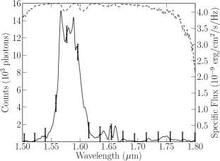
Figure 2.— A smoothed model spectrum for an atmosphere with $T_{\rm eff}=400$ K and $\log(g)=3.66$ is shown as a solid black line, with black points indicating where the spectrum is sampled, and system noise in each channel as solid black bars. This is representative of a 4 $M_{J}$ planet around a 500 Myr Sun-like star 40 parsecs from Earth. The dashed black line shows terrestrial atmospheric transmission.

4. Planet Models

We consider planets without internal energy sources (i.e., deuterium fusion) that are young and sufficiently far from their primary star that we can ignore the stellar radiation field when considering cooling and contraction, i.e., $T_{\rm eff}$$>>(R_{*}/a)^{1/2}T_{*}$, or $T_{\rm eff}$${}^{4}>>(180K)^{4}$ for a planet orbiting a solar type star at $a=5$ AU.

The luminosity of a planet is given by its radius and effective temperature, but the detectability at specific wavelengths also depends on the nature of the dominant opacity sources in the photosphere. The photospheric chemical composition at a given effective temperature is sensitive to surface gravity, $g=GM/R^{2}$. Both $T_{\rm eff}$ and $\log(g)$ are depend upon the age and the mass of the planet. To understand the detectability of a planet then involves converting a planet age and mass to a luminosity, effective temperature, radius, and surface gravity.

To establish this mapping, we compare two evolutionary models. One is the so called “hot start” model of Burrows et al. (1997), and the other is the the core accretion model of Marley et al. (2007). The most significant difference between the two is summarized in Figure 3, which shows effective temperature and surface gravity for different mass and age contours. While the expected effective temperatures and surface gravities of the two models come in to rough agreement for older planets, planets that form via core accretion are expected to be significantly cooler post-formation than planets formed via a hot start.

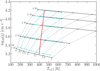
Figure 3.— Surface gravity plotted against effective temperature for selected mass and age contours for two planet formation models, where contours are labeled in $M_{J}$ and $\log(t)$. The Burrows et al. (2003) hot start model is shown in black, and the Marley et al. (2007) core accretion model is in cyan. The H₂O condensation line is shown in red, below which planet atmosphere calculations become more uncertain. The position of Jupiter, at $T_{\rm eff}\approx 125$ K, $\log(g)\approx 3.4$, and $\log(t)\approx$ 9.66, is shown as a magenta dot.

4.1. Hot start models

The label “hot start” was used by Marley et al. (2007) to describe models of the atmospheres and evolution of extrasolar giant planets that ignored the different formation mechanisms of brown dwarfs and gas giants. These models assumed that an object’s mass, age, and composition dominated its spectral characteristics, and assumed that gas giant planets, like brown dwarfs, form like stars. Objects formed in this manner possess a fully adiabatic interior with high specific entropy, which corresponds to a high internal temperature. These models focus on treating the atmospheres of gas giant planets in order to predict the emergent flux as a function of temperature and surface gravity.

The hot start model used here is that of Burrows et al. (1997), which spans an effective temperature range from approximately 100 K to 1000 K, covering the realm between the known Jovian planets and the known T dwarfs. The models can be conveniently approximated as power laws, found by performing a regression over a restricted range of masses and ages of interest: 1 $<$ $M/M_{J}$ $<$ 12 and 0.01 $<$ t/Gyr $<$ 2. The resultant expressions are

$$T_{\rm eff}(M,t) = (145\;K)\left(\frac{t}{{\rm Gyr}}\right)^{-0.29}\left(\frac{M}{M_{J}}\right)^{0.47},$$ (1)

$$L(M,t) = (5.4\times 10^{-9}L_{\odot})\left(\frac{t}{{\rm Gyr}}\right)^{-1.21}\left(\frac{M}{M_{J}}\right)^{1.87},$$ (2)

$$R(M,t) = (1.13R_{J})\left(\frac{t}{{\rm Gyr}}\right)^{-0.034}\left(\frac{M}{M_{J}}\right)^{-0.013}.$$ (3)

These expressions are comparable to previous semiempirical estimates of these dependences (Black, 1980), and the luminosity expression is close to that of cooling at constant heat capacity ($L\sim M^{2}t^{-4/3}$). The resultant radii and effective temperatures have rms errors of 2% and 4% respectively. The corresponding error in bolometric magnitudes is 0.15 mag. We use the radiative-convective equilibrium atmosphere model of Marley et al. (1996), further described in Burrows et al. (1997); the most recent tabulations are provided in Burrows et al. (2003). The model has been updated to self-consistently include both alkali opacities Burrows et al. (2000) and precipitating clouds (Ackerman & Marley, 2001).

A major source of uncertainty in planet atmosphere models is the treatment of clouds. As with the known T and L dwarfs, absorption by water vapor dominates the spectra of the cooler brown dwarfs. These features generally deepen with increasing age and decreasing mass. This trend is in part due to the increase with decreasing gravity of the column depth of water above the photosphere. At effective temperatures below 400–500 K, water vapor condenses in planetary atmospheres. The appearance of water-ice clouds constitutes a major uncertainly separating the known T dwarfs from the giant planets, and is denoted in Figure 3. When water condenses, water vapor is depleted above the cloud tops causing a decrease at altitude in the gas-phase abundance of water. Water clouds form in the atmosphere of an isolated 1 $M_{J}$ object within 100 Myr, and within 2 Gyr they form in the atmosphere of a 12 $M_{J}$ object. However, at supersaturations of 1% and for particle sizes above 10 $\mu$m, such clouds (and the corresponding water vapor depletions above them) only marginally affect the calculated emergent spectra. For wavelengths long-ward of 1 $\mu$m, the cloudy spectra differ from the no-cloud spectra by at most a few tens of percent. Below effective temperatures of 160 K, NH₃ clouds form. This is likely well below the effective temperature we can hope to detect.

We expect that planets detected in reflected light will comprise only a negligible fraction of our sample, and therefore we have not attempted a thorough treatment of this problem. Rather, we assume a Bond albedo of 0.4. This assumption would gives rise to errors if the observing band were coincident with a strong CH₄ band or when the target it is a so-called Class III or “clear” extrasolar giant planet, so named because they are expected to be too hot ($T_{\rm eff}$$\geq$ 350 K) to contain any principal condensates (Sudarsky et al., 2000).

4.2. Core accretion

The standard theory for the formation of gas giant planets is the core accretion model (e.g., Pollack et al. 1996), which begins with dust particles colliding and agglomerating within a protoplanetary disk to form icy and rocky planetary cores. If the core becomes massive enough while gas remains in the disk, it can grow by gravitational accretion of this gas. Gas giants accrete most of the gas within their tidal reach, filling the Hill sphere around them with a hot, extended, gaseous envelope. Further accretion is slowed by the dwindling supply of local raw materials and by the extended envelope, leading to growth times of 5–10 Myr. The predicted planet formation time is uncomfortably long compared to the observed $\sim$ 3 Myr lifetime of protoplanetary disks. Two factors may alleviate this time-scale problem: 1) inward migration can bring giant planets to fresh, gas-rich regions of the disk; 2) dust sedimentation may reduce atmospheric opacity, which leads to more rapid escape of accretion luminosity and shrinkage of the envelope. Hubickyj et al. (2005) have shown that reducing the grain opacity to a level observed in L dwarfs (Marley et al., 2002) reduces the planet growth time scale to $\sim$ 1 Myr, well within the lifetime of protoplanetary disks. Once accretion stops, the planet enters the isolation stage and the planet contracts and cools at constant mass.

The configuration of the protoplanet at the end of run-away gas accretion represents the initial conditions for subsequent cooling and contraction. Marley et al. (2007) and Fortney et al. (2008) have conducted preliminary calculations that describe the cooling and contraction of a young planet as it emerges from its parent disc. The implication of the Marley et al. (2007) results is that giant planets formed by core accretion are less luminous post-accretion than had been previously expected because significant energy is radiated during the formation process. The fully formed planet has a smaller radius at young ages than hot start models predict (Burrows et al., 1997; Baraffe et al., 2003), leading to a lower post-formation luminosity. There are two significant observational consequences: 1) there is a period of very high luminosity ($\sim$ 10^-2 L_⊙) which lasts $\sim$ 40,000 yr; 2) the initial conditions for subsequent evolution are not “forgotten” for a time of order the Kelvin-Helmholtz timescale, which lasts tens of millions of years. These factors imply that observations of class II (0.5–3 Myr) and III ($\sim$ 10–100 Myr) young stellar objects afford the opportunity to probe the planet formation events. The run-away accretion spike is likely to be broader and fainter than in these idealized calculations because of gradual accretion across the gap that the protoplanet forms, and the probability of witnessing this event in a typical T Tauri star may be much larger than a few percent

The approximations used to compute the luminosity history of a planet formed by core accretion are similar to those adopted in early studies of protostellar formation—the runaway gas accretion phase is described using the formalism of Stahler et al. (1980), where matter falling onto the central object passes through a 1-d, optically thick shock. The 1-d geometry forces all the matter to pass through this shock, whereas in nature the accretion is at least 2-d and more realistically 3-d. Comparison with star formation suggests that some accretion may occur on viscous time scales in a disk rather than on the fast dynamical timescale depicted in Fortney et al. (2008). Ultimately, the virial theorem must be satisfied, and half the gravitational potential energy is radiated: the Marley et al. (2007) calculations and the hot start models (Burrows et al., 1997; Baraffe et al., 2003) represent limiting cases in the contraction history.

Despite the preliminary nature of the Marley et al. (2007) results, one message is clear: the luminosity of young exoplanets encodes key information about how they were formed. Simulations suggest that the timescales for relaxation are longer for more massive planets, and are at least approximately related to the Kelvin-Helmholtz timescale, with

$$\tau\sim\frac{GM^{2}}{RL},$$ (4)

where $G$ is the gravitational constant, $M$ is the mass of the planet, $R$ is the radius of the planet, and $L$ is the luminosity of the planet. This timescale ranges from tens to hundreds of millions of years for gas giants, meaning observations of stars with ages in this range will yield information about planet formation. Young targets are also the most promising targets because a brighter planet is more easily detected, but planets formed via core accretion may be cooler at young ages than hot start planets. If planets are significantly cooler at young ages than hot start models assumed, the detection rate of young gas giants will be lower than expected.

5. Observation planning

5.1. Planet populations & Monte Carlo simulations

We use the results of the sensitivity calculations described in Section 3 and the planet formation and atmosphere models described in Section 4 to perform Monte Carlo simulations characterizing the results of different surveys using the Gemini Planet Imager (Graham et al., 2002; Graham, 2007; Graham et al., 2007). The sensitivity of the instrument to a planet depends upon the angular separation between the host star and planet and the brightness of the host star. The spectrum of a planet depends on its effective temperature and surface gravity, which themselves are functions of the mass and age of the planet. Specifying the mass, age, and orbital elements of a planet and the brightness and distance of its host star is then sufficient to determine whether that planet is detectable according to the model used. By generating distributions of the orbital elements and mass of exoplanets, and assuming that planet and host star formation are coeval, we may then simulate the likelihood of detecting a planet around some star.

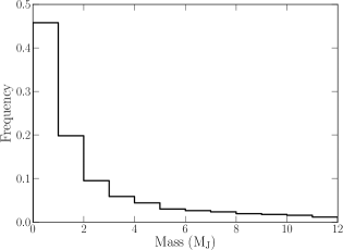
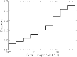
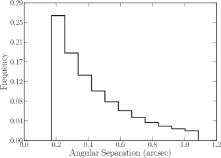
Figure 4.— Distributions of planet properties in a typical survey. The mass and semi-major axis distributions are drawn from extrapolations of distributions consistent with radial velocity detected planets. The angular separation distribution assumes a population of host stars distributed randomly in a volume within 100 parsecs of the Sun. The effective temperature distribution assumes a distribution of stellar ages based on a simple galactic disk star formation rate, and that planet mass and age map to effective temperature as described in Marley et al. (2007).

Lacking an accepted paradigmatic theoretical model for the distributions of these parameters, we rely on the distributions at semi-major axes smaller than $\sim 5$ AU found via radial velocity surveys, and extrapolate these distributions to larger semi-major axes. The applicability of the mass and eccentricity distributions found for close-in companions at large semi-major axes is unclear, as is the extension of the semi-major axis distribution to larger semi-major axes. Nevertheless, as a baseline we apply recent results that indicate that the planet mass and semi-major axis each follow a power law distribution, with $dN/dM\propto M^{-1.31}$ and $dN/da\propto a^{-0.61}$ (Cumming et al., 2008). For the mass, we adopt a lower cutoff of 0.5 $M_{J}$, below which a planet is so dim as to make direct imaging unlikely, and below which radial velocity surveys are incomplete. We take as an upper cutoff 12 $M_{J}$, reflecting the transition from planet to brown dwarf at the deuterium fusion limit, thereby ignoring any details of how the planet formed. A histogram of planet masses sampled from this distribution is shown in the upper left panel of Figure 4.

Similarly, we adopt cutoffs for the the semi-major axis distribution of 0.1 AU and 75 AU. Radial velocity surveys show a rising power law for the semi-major axis distribution in log space out to $\sim 5$ AU, and Nielsen et al. (2010) placed an upper limit of 75 AU on the semi-major axis distribution quoted in Cumming et al. (2008). A lower cutoff may be justified, but already detected exoplanet systems, such as Fomalhaut, HR 8799, and 1RXS J160929 indicate that some planets form at large semi-major axes. Such a cutoff is also consistent with the typical sizes of T Tauri disks (Isella et al., 2009). A sampled population from this distribution is shown in the upper right panel of Figure 4.

The eccentricity distribution is also drawn from radial velocity observations. Over a decade ago, an eccentricity distribution of $dN/de\propto e^{-0.5}$ was proposed by Heacox (1999), but to our knowledge, no updated eccentricity distribution has been published. We found that a simpler linear fit to eccentricities adequately describes observations to date, and adopted that, as results are insensitive to the eccentricity distribution anyway. The rest of the orbital elements are easily obtained. The mean anomaly and the argument of perihelion are both drawn from a uniform distribution from 0 to 2$\pi$. The inclination of the orbit relative to the plane of the sky is drawn from a distribution of randomly oriented orbits, i.e. $dN/di=\frac{1}{2}\sin(i)$.

With these distributions, we use a pseudo random number generator and the rejection method to generate a population of exoplanets, which may be placed around some star. The distribution of masses is then converted to distributions of surface gravity, radius, and temperature according to the adopted formation model, and the temperature and surface gravity then give the emergent spectrum of the planet, as described in Section 4. From this, an expected flux at the telescope in each spectral channel is calculated. Per the discussion in Section 3.4, these channels may be summed with our without weights to get a total flux across the band, but in all results here channels are summed without weights. Finally, the distributions of orbital parameters yield a distribution in angular separation. For a given star, we then have relative brightnesses as a function of angular separation, which can be compared with the expected performance of GPI. The probability of detecting a planet around a star, assuming a single planet with mass $0.5M_{J}<M<12M_{J}$, is then directly obtained from the percentage of relative brightnesses across the entire wavelength band that are above the threshold of detectability, which is taken to be a signal to noise ratio of 5.

Known exoplanets suggest that these distributions should depend on the properties of their host star. The observed metallicity dependence for short period planets has already been discussed in Section 1, but will not be included in any simulations due to uncertainty in its applicability at large semi-major axes. Doppler surveys show that the fraction of stars with planets increases with stellar mass over the range from M to A stars (Johnson et al., 2008). Microlensing results for the distribution of planets beyond the ice line are in terms of the mass ratio distribution $dN/dq$, where $q=M_{p}/M_{s}$, rather than a simple distribution of masses $dN/dM$. The success at finding planetary mass companions around A stars with other direct imaging efforts also supports the importance of host star mass, even at large semi-major axes (e.g., Fomalhaut and HR 8799). Gorti et al. (2009) predict that the disk lifetime is relatively constant for $M\leq 2M_{\odot}$, which is also consistent with the notion that Jupiter mass planets are more common around A stars than they are around M stars. To explore the impact of host star mass on direct imaging surveys, we tested both a mass ratio distribution $dN/dq$ and a simple mass distribution $dN/dM$. The mass power law index given in Cumming et al. (2008) was also used for the mass ratio distribution, so that $dN/dq\propto q^{-1.31}$. The upper and lower cutoffs for $q$ are set such that the lower mass cutoff is 0.5 $M_{J}$ and the highest mass is 12 $M_{J}$, for the same reasons those cutoffs are adopted for the $dN/dM$ distribution. This is unsubstantiated quantitatively, but seems reasonable qualitatively. For the rest of the paper, we note when results are for a mass ratio distribution.

Due to incompleteness, Doppler surveys have not yielded an absolute planet hosting probability. Nevertheless, Cumming et al. (2008) estimate that 17–20% of FGK stars host planets with $M>0.3M_{J}$ and with $a<20$ AU. Surveys using Spitzer IRAC and MIPS find debris disks around  15% of solar-type stars younger than 300 Myr Carpenter et al. (2009) and around  33% of A-type stars Su et al. (2006) younger than 850 Gyr, suggesting a lower limit of this order for the probability of hosting a planet. We generally sidestep the uncertainty in planet hosting probabality by reporting the detection rate in terms of the ratio of the number of planets detected to the total number of planets. When reporting the total number of planets detected around a sample of a fixed number of stars, we adopt the simple assumption that all stars host a single planet more massive than 0.5 $M_{J}$ in the range 0.5–70 AU.

5.2. Simulated surveys

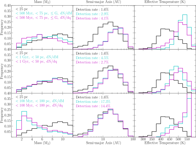
Figure 5.— Each row of panels plots the intrinsic mass, semi-major axis, and temperature distributions of detected planets from three different surveys. The target selection criteria for the three surveys in each row are given by the matching color text in the left column, and the total detection rate for the survey is given in the middle column. The black line is the same in all rows, showing a volume limited selection. Within each row, the cyan and magenta lines represent the same target selection criteria, but are distinguished by whether planet mass depends upon host mass. For cyan lines, planet mass is independent of host mass, while planet mass scales proprotionally to host mass for the magenta lines. Cyan and magenta lines are for a survey emphasizing massive stars in the top row, a survey emphasizing nearby stars in the middle row, and a survey emphasizing young stars in the bottom row.

Simulating a survey is a straightforward extension of simulating the likelihood of detecting a planet around a single star. Two of the authors independently wrote code to do this, and used slightly different approaches. In one approach, a sample population of planet properties was drawn from the distributions described in the previous section and then placed it around each star in some sample of stars. In the other approach, a new sample population of planet properties was created for each star. The results of these two approaches were in excellent agreement, providing confirmation that neither code contained major errors, and the choice of using the same planet property distribution for each star or different ones was unimportant to the results for simulated surveys with a large number of planets.

The stellar sample used in a simulation may be either a list of real stars, or a Monte Carlo population, where stellar masses are generated from a Kroupa IMF, stellar ages are based on a simple galactic disk turn-on and turn-off, and stellar distances are generated to match the observed stellar density in the solar neighborhood (Kroupa, 2001; Mihalas & Binney, 1981). In either case, the same procedure for simulating the likelihood of detecting a planet around a single star may be used for a number of stars. For different stars, the primary factors that change are the angular separation on the sky of star and planet, the brightness of the star, and the brightness of a planet of given mass, as planet brightness depends upon the age of the system. A record is kept of the planets that are detectable around each star.

Performing a simulation over a sample of stars provides a total detection rate and a distribution of properties for detected planets. These may be used to compare surveys emphasizing different target selection, which may then inform where target identification efforts should be focused. With this in mind, we simulated a population of stars within 100 parsecs, and then performed three surveys for samples where targets were selected based on different sets of criteria. These criteria were age, distance, and spectral type (or mass), and the results are shown in Figure 5. To provide a fair comparison between the surveys, the criteria adopted for each survey were chosen to yield roughly the same number of available targets in each survey. The distributions plotted assume complete information about the planet detected, which will obviously not be the case for real planets; while the semi-major axis and effective temperature may be derived from observations directly, determining the mass of a planet from direct observations will generally require planet formation and atmosphere models, or dynamical constraints for multi-planet systems or planets in disks.

The results in Figure 5 show that observing young stars that are even reasonably near the Sun may be expected to yield the highest detection rates, as well as the most information about planets at the lower end of the mass distribution. The primary drawback in observing the youngest stars is that it requires observing stars at greater distances. The inner edge of the “dark hole” region is roughly 0.2″, so only planets outside of 20 AU may be observed for a star that is 100 parsecs distant. If gas giants are very rare at semi-major axes greater than 20 AU or so, selecting only young stars would lead to a significantly diminished detection rate. Selecting for stars that are somewhat older and nearer is not as successful in detecting planets for the semi-major axis distribution that we have assumed, as the gas giants with masses $\sim M_{J}$ and ages $\sim$ Gyr are too dim to detect in an hour observation in most cases. Such a survey choice does have the advantage that the majority of detected planets are at semi-major axes $<$ 20 AU, and the existence of gas giants at 5–20 AU is somewhat better established than the existence of gas giants from 30–70 AU. Present efforts to identify targets for GPI are focused primarily on young stars, but very nearby stars that also happen to be only moderately young are promising targets as well. The desirability of early type stars depends on how the planet mass distribution depends upon stellar mass. Under the assumption that the planet mass distribution is independent of stellar mass, later type stars have the highest planet detection rate, since for the same age and planet mass, the ratio of planet brightness to star brightness will be higher for dimmer stars. Planet mass very likely does depend on host star mass, and making the simple assumption that planet mass scales linearly with host star mass, planet detection rates are highest for early type stars. This result suggests a continued emphasis on identifying early type stars will be valuable to a successful direct imaging survey.

Another means of survey comparision is the completeness diagram, which encapsulates information about both the rate of detection and the properties of the planets detected, showing for a grid of planet masses and semi-major axes the fraction of planets that are detected. Two samples are shown in the completeness diagram in Figure 6, with one sample limited to stars younger than 100 Myr, and the other limited to stars younger than 1 Gyr and nearer than $50$ pc. The young star sample was taken from catalogs assembled by I. Song and M. Bessell (private communication). Recognizing the importance of a large target set of young, nearby stars (defined as age $\leq$ 100 Myr and distance $\leq$ 75 pc), Song and Bessell initiated a large-scale program in 2007 to identify and characterize young stars. There are approximately 200 known nearby young stars ($\leq$ 75 pc; $\leq$ 100 Myr) in the literature (e.g., Zuckerman & Song 2004; Torres et al. 2006). To find new candidate young stars, Song and Bessell selected about 3000 bright ($I\leq$ 9 mag.) Tycho-2 stars from ROSAT catalogs with enhanced X-ray emission and potential young star kinematics and obtained optical echelle spectra of about 2000 high priority targets with the 2.3-m at Siding Spring. These spectra were used to extract age indicators including Li 6708 $\AA$, Ca II HK, H$\alpha$, and $v\sin(i)$ and estimated ages following Zuckerman & Song (2004), yielding about 200 additional young stars. When combined with an unpublished list of nearby young stars (400; Song, Zuckerman, and Bessell since 2000) and currently known members of nearby young stellar groups (400), there are approximately 1000 distinct solar-type stars that are 100 Myr old or younger within 75 pc. There are also more than 1000 “adolescent” stars (100–500Myr.) Age uncertainties in the age-dating methods used are age dependent (smaller for younger ages) and $\pm$5 Myr for the youngest stars ($\sim$10 Myr old) and $\pm$300 Myr for the oldest stars (500 Myr). The sample used here is limited to roughly 600 stars accessible to the Gemini South telescope, and has a median age of $~{}50$ Myr and median distance of $~{}50$ pc. The mean age and distance of the sample are both $~{}20$% larger than the median. The other sample consists of stars from the Geneva-Copenhagen survey (Holmberg et al., 2009), which was chosen because it is a publically available catalog of stars with estimated ages and distances. From the Geneva-Copenhagen catalog, we selected stars accessible to Gemini South that are younger than 1 Gyr and nearer to the Sun than $50$ pc, of which there are roughly 200. The diagram shows that a survey of moderately young and nearby stars will probe a reasonable fraction of mass and semi-major axis space, but only by surveying a very young sample of stars is there a significant probability of imaging gas giants with $M\sim M_{J}$. There is, however, a reasonable likelihood of detecting the more massive gas giants around adolescent stars, and detection of the most massive planets will be limited primarily by the fraction the orbit during which the planet is in the “dark hole” observing region of GPI.

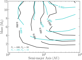
Figure 6.— Completeness diagram comparing two surveys that assume planets evolve according to the models of Marley et al. (2007). The cyan represents detection rates for a survey of stars within 50 parsecs and younger than 1 Gyr target stars from the Geneva-Copenhagen Survey (Holmberg et al., 2009), while the black lines are for a survey of young stars (age $<$ 100 Myr) from a target list being compiled for GPI (Song and Bessell, private communication). The colors of the text correspond to the same surveys, and show the number of stars surveyed $N_{*}$ and the number of detected planets $N_{p}$, assuming one planet per star.

5.3. Target Ordering

In simulated surveys, a planet detection probability is recorded for each star. These detection probabilities are some function of the star’s age, distance, and spectral type. We find this function can be approximated reasonably well with a product of power laws when considering only stars younger than 2 Gyr. For an older sample, the large number of stars with effectively zero probability of observing a planet can skew the resulting fit. Denoting the star’s age by $t$, distance $d$, and mass $M$, the detection probability $p$ is

$$p=A\left[\log{\left(\frac{t}{{\rm 1\;Myr}}\right)}\right]^{\alpha}\left(\frac{d}{{\rm 40\;pc}}\right)^{\beta}\left(\frac{M}{M_{\odot}}\right)^{\gamma},$$ (5)

with the parameters scaled to appropriate values to ease fitting, and the logarithm of the age being used as the ages for young stars are known with precision at the order of magnitude level. Performing this regression over multiple trials, and assuming that planet planets are described by the models of Marley et al. (2007) and that mass is independent of stellar mass, we find $\alpha\sim-5$, $\beta\sim-1.5$, $\gamma\sim-1.5$. While the best fit values are sensitive to the average age of stars in a sample, they emphasize priority in the same general way: the log of the age is the most important parameter, and the distance and mass of the star are of roughly equal importance.

Once generated, this detection probability function can be used to order target selection before GPI begins observations, as well as for ordering targets in new simulated surveys. This application is demonstrated in Figure 7, which shows the results of two surveys of 1000 stars limited in age to be younger than 1 Gyr. If all stars in the sample are observed, the end result is the same, but when ordering the targets, approximately 2/3 of detectable planets are found in the first 1/3 of the sample.

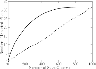
Figure 7.— The expected number of detected planets is shown for two observing strategies. The dashed black line indicates targets chosen randomly from a sample of stars younger than 1 Gyr and within 70 parsecs. The solid black line shows the results when the targets are ordered according to Equation 5.

Fitting for the target ordering parameters also gives an at-a-glance sense of what is important in a survey. As such, it is an interesting way to test the impact of assumptions about the planet population. For instance, when the distribution $dN/dq$ is used rather than $dN/dM$ for generating planet masses, detection probability increases with host star mass rather than decreasing. The other parameters stay roughly the same, with $\alpha\sim-5,\beta\sim-1.5,\gamma\sim 1$. Likewise, changing the slope on the semi-major axis distribution unsurprisingly impacts the importance of stellar distance on a survey.

6. Expected GPI Performance

6.1. Detection rate and distributions

With 150 nights of telescope time, GPI could perform initial 1 hour observations and follow-up for roughly 1000 stars. The results of such a survey depend strongly on target selection. The predictions of the formation model also strongly influence an exoplanet survey, though this effect decreases as the mean age of targets increases and model predictions converge. An age limited survey of stars younger than 1 Gyr within 80 parsecs will have a detection rate of 4% for the Marley et al. (2007) model, whereas planets that evolve according to Burrows et al. (2003) will be detected around 12% of stars. For a survey of the stars younger than 100 Myr being compiled by Song (2010, private communication) for GPI, and with the important assumption that the semi-major axis distribution observed for radial velocity exoplanets continues out to $\sim$ 70 AU, these detection rates increase to 13% and 21% for the Marley et al. (2007) and Burrows et al. (2003) models, respectively. For a volume limited survey of very nearby stars, the detection rate drops to 1–2% for both models.

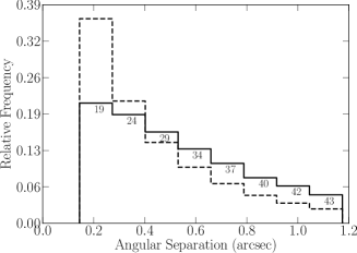
Figure 8.— The distribution of angular separation for GPI detected planets is shown by the solid black line, while the distribution for generated planets is shown by the dashed black line. The average semi-major axis of planets within each bin is printed at the top of the bin.

While the existence of a significant population of planets at large semi-major axes (30–70 AU) will certainly improve the detection rate of a GPI survey, GPI may still be successful so long as gas giants exist at more moderate semi-major axes. GPI is capable of detecting planets separated by less than $0.2\arcsec$ from their hosts. This is illustrated by Figure 8, which shows the distribution of angular separation for planets detected by GPI, as well as the intrinsic angular separation distribution, given the assumed semi-major distribution and distribution of stellar distances. The majority of detected planets will come from the inner half of the GPI “dark hole.” For the innermost angular separation bin, the average semi-major axis of detected planets is 18 AU. These small separations are where GPI will be most valuable, probing regions of semi-major axis space inaccessible to previous imaging surveys. Figure 8 also indicates that regardless of the number of planets at large semi-major axes, GPI will probe a region of semi-major axis space which has been unexplored by previous radial velocity surveys and direct imaging surveys.

Likewise, GPI is capable of detecting a wide range of planet masses. As shown in Figure 5, observations of young stars may be expected to yield detections of planets with mass $M\sim M_{J}$ in reasonable numbers. For planets with mass $M\sim 8M_{J}$ and above and ages less than 1 Gyr, the detection rate is limited primarily by fraction of an orbit that planets spend in the “dark hole” region. This remains true for objects beyond the deuterium burning demarcation between planets and brown dwarfs. Imagining the planetary mass distribution extending to the realm of low-mass brown dwarfs up to 30 $M_{J}$, GPI could expect to find at least twice as many brown dwarfs as planets. It should quickly become clear whether the brown dwarf desert extends to large semi-major axes.

6.2. Model differentiation

The core accretion model of Marley et al. (2007) and the hot start model of Burrows et al. (2003) make distinct predictions for the expected properties of young gas giants. The differences in formation models are greatest for the planets that are young, so a survey targeting stars with ages $\sim 100$ Myr and younger is most effective. If gas giants were were formed via only one of the two scenarios, conducting a survey of 100 stars with these ages would be sufficient to determine which model described the formation of the planets. We performed a simulated survey like this twice, once for each model. Figure 9 shows the expected results of such each survey, with effective temperatures of detected planets as a function of planet age. It is clear that the two populations of planets are very different, both to the eye and from performing simple statistical tests comparing the distributions and their agreement with each of the models. For this simple scenario then, a modest amount of observing time can distinguish the two formation models.

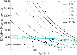
Figure 9.— Effective temperatures of detected planets are shown as a function of planet age as circles, with representative error bars in the lower left corner. Black circles indicate planets with properties according to the model of Burrows et al. (2003), and cyan circles correspond to planets from the Marley et al. (2007) model. The lines show expected planet cooling tracks for each model for planet masses of 1, 2, 4, 6, 8, and 10 $M_{J}$, and the colors for the cooling tracks are black for Burrows et al. (2003) and cyan for Marley et al. (2007). More massive planets are at most ages warmer than less massive planets in each model, but the Marley et al. (2007) planets all converge to roughly the same temperature at young ages.

In reality, this dichotomy will not exist. The models represent two extreme cases, and the post formation entropy of any individual planet would likely fall somewhere in between what each of the models predicts. Looking at a distribution of planets will be even more complicated if planets form via more than one mechanism. It will likely be valuable to segregate distributions of detected planets by semi-major axis, host mass, and planet metallicity, according to predictions about how the planet distribution will depend upon these stellar properties for each formation mechanism. Significant differences in these segregated distributions could provide useful evidence for a difference in formation history.

In simulating formation model differentiation, the other major simplification was ignoring the existence of brown dwarfs, which will also likely complicate efforts to determine how planets form. Well constrained stellar ages will be vital in discriminating between planet formation models. Objects that are brown dwarfs according to both the deuterium fusion limit and in the sense of forming like a star are expected to be significantly warmer and more luminous than planet mass objects at the same age. Objects with masses above the deuterium burning limit that formed via core accretion are potentially more problematic if their post formation luminosities are similar to planet mass objects that formed through core accretion. However, the surface gravities of objects above and below the deuterium burning limit will be different enough to be distinguished, as GPI is expected to achieve a precision of better than 0.2 dex in $\log(g)$.

The HR 8799 system provides an early example of examining planet formation models using the effective temperatures and ages of detected planets. As noted in Marois et al. (2008a), the members of the HR 8799 system are not consistent with the simple core accretion model presented in Marley et al. (2007). After the formation event, planets formed in their model are insufficiently hot to match the temperatures of the HR 8799 members, even considering the large uncertainty in the age of the planets. Given the dynamical constraints on the system that place an upper limit on the masses of $\sim 10M_{J}$ (Fabrycky & Murray-Clay, 2010), and despite the fact that the thermal history of a planet formed via core accretion is undoubtedly more complicated than the model presented by Marley et al. (2007), the temperatures of the HR 8799 planets support the notion that planets do not form by core accretion at large semi-major axes. The observed abundance of multi-planet systems suggests that some of the planets GPI will discover will also be in multi-planet systems. Finding more systems like HR 8799 will help determine more confidently how planets form.

7. Conclusions

We have simulated the performance of the Gemini Planet Imager in a variety of hypothetical direct imaging surveys of nearby stars, finding how the detection rate and properties of detected planets are affected by different survey choices and assumptions about the exoplanet distribution. These simulations rely upon calculations and simulations of the noise properties of the system. They also rely upon models of the formation and evolution of gas giant planets and their atmospheres, one assuming a hot start (Burrows et al., 2003) and one assuming a planet formed by core accretion (Marley et al., 2007).

Regardless of formation model, detection rates will be highest for observations of young stars. For planets that formed via core accretion, roughly 10% of planets around stars younger than 100 Myr may be detected, and for hot start planets this detection rate may be as high as 25%. One major uncertainty is the frequency of planets at large semi-major axes. If planets are very rare beyond 30 AU, a GPI survey would be more successful focusing on moderately young nearby stars, rather than the youngest stars. Only by sampling the youngest stars though may GPI be expected to place significant constraints on the low-mass end of the semi-major axis distribution, as the least massive planets cool the most quickly, and sampling young stars will also be the most useful approach to better understanding how planets form.

For planets detected with reasonably high signal to noise, GPI will be capable of measuring the effective temperature and surface gravity. When the age of the system is known, these quantities can be compared to models of planet formation and evolution. For the idealized situation where all planets are formed via either the hot start model of Burrows et al. (2003) or the core accretion models of Marley et al. (2007), a few tens of detected planets younger than 100 Myr would be sufficient to determine the model from which the planets were drawn. Real planets will not be so simple, but this result suggests that the characterization of many planets in this fashion will lead to a better understanding of how planets form.

We would like to acknowledge Jonathan Fortney, Mark Marley, and Didier Saumon for helpful discussion regarding their models and for providing additional model spectra at our request.

References

- Ackerman & Marley (2001) Ackerman, A. S., & Marley, M. S. 2001, ApJ, 556, 872
- Anglada-Escudé et al. (2010) Anglada-Escudé, G., Shkolnik, E. L., Weinberger, A. J., Thompson, I. B., Osip, D. J., & Debes, J. H. 2010, ApJ, 711, L24
- Anic et al. (2007) Anic, A., Alibert, Y., & Benz, W. 2007, A&A, 466, 717
- Apai et al. (2008) Apai, D., et al. 2008, ApJ, 672, 1196
- Armitage et al. (2002) Armitage, P. J., Livio, M., Lubow, S. H., & Pringle, J. E. 2002, MNRAS, 334, 248
- Baraffe et al. (2003) Baraffe, I., Chabrier, G., Barman, T. S., Allard, F., & Hauschildt, P. H. 2003, A&A, 402, 701
- Bean et al. (2010) Bean, J. L., Seifahrt, A., Hartman, H., Nilsson, H., Reiners, A., Dreizler, S., Henry, T. J., & Wiedemann, G. 2010, ApJ, 711, L19
- Berdyugina et al. (2008) Berdyugina, S. V., Berdyugin, A. V., Fluri, D. M., & Piirola, V. 2008, ApJ, 673, L83
- Beuzit et al. (2010) Beuzit, J., et al. 2010, in Astronomical Society of the Pacific Conference Series, Vol. 430, Astronomical Society of the Pacific Conference Series, ed. V. Coudé Du Foresto, D. M. Gelino, & I. Ribas, 231–+
- Biller et al. (2007) Biller, B. A., et al. 2007, ApJS, 173, 143
- Black (1980) Black, D. C. 1980, Icarus, 43, 293
- Boley (2009) Boley, A. C. 2009, ApJ, 695, L53
- Borucki et al. (2003) Borucki, W. J., et al. 2003, in Presented at the Society of Photo-Optical Instrumentation Engineers (SPIE) Conference, Vol. 4854, Society of Photo-Optical Instrumentation Engineers (SPIE) Conference Series, ed. J. C. Blades & O. H. W. Siegmund, 129–140
- Borucki et al. (2011) Borucki, W. J., et al. 2011, ArXiv e-prints
- Boss (2002) Boss, A. P. 2002, ApJ, 576, 462
- Burrows et al. (2000) Burrows, A., Marley, M. S., & Sharp, C. M. 2000, ApJ, 531, 438
- Burrows et al. (2003) Burrows, A., Sudarsky, D., & Lunine, J. I. 2003, ApJ, 596, 587
- Burrows et al. (1997) Burrows, A., et al. 1997, ApJ, 491, 856
- Butler et al. (2006) Butler, R. P., et al. 2006, ApJ, 646, 505
- Carpenter et al. (2009) Carpenter, J. M., et al. 2009, ApJS, 181, 197
- Casertano et al. (2008) Casertano, S., et al. 2008, A&A, 482, 699
- Charbonneau et al. (2005) Charbonneau, D., et al. 2005, ApJ, 626, 523
- Chiang et al. (2002) Chiang, E. I., Fischer, D., & Thommes, E. 2002, ApJ, 564, L105
- Cumming et al. (2008) Cumming, A., Butler, R. P., Marcy, G. W., Vogt, S. S., Wright, J. T., & Fischer, D. A. 2008, PASP, 120, 531
- Dodson-Robinson et al. (2009) Dodson-Robinson, S. E., Veras, D., Ford, E. B., & Beichman, C. A. 2009, ApJ, 707, 79
- Ercolano & Clarke (2010) Ercolano, B., & Clarke, C. J. 2010, MNRAS, 402, 2735
- Fabrycky & Murray-Clay (2010) Fabrycky, D. C., & Murray-Clay, R. A. 2010, ApJ, 710, 1408
- Fischer & Valenti (2005) Fischer, D. A., & Valenti, J. 2005, ApJ, 622, 1102
- Fortney et al. (2008) Fortney, J. J., Marley, M. S., Saumon, D., & Lodders, K. 2008, ApJ, 683, 1104
- Fressin et al. (2010) Fressin, F., Knutson, H. A., Charbonneau, D., O’Donovan, F. T., Burrows, A., Deming, D., Mandushev, G., & Spiegel, D. 2010, ApJ, 711, 374
- Gammie (2001) Gammie, C. F. 2001, ApJ, 553, 174
- Goldreich et al. (2004) Goldreich, P., Lithwick, Y., & Sari, R. 2004, ARA&A, 42, 549
- Goldreich & Sari (2003) Goldreich, P., & Sari, R. 2003, ApJ, 585, 1024
- Goldreich & Tremaine (1980) Goldreich, P., & Tremaine, S. 1980, ApJ, 241, 425
- Gorti et al. (2009) Gorti, U., Dullemond, C. P., & Hollenbach, D. 2009, ApJ, 705, 1237
- Gould et al. (2010) Gould, A., et al. 2010, ArXiv e-prints
- Graham (2007) Graham, J. R. 2007, Gemini Planet Imager Operational Concept Definition Document V3.2 (Hilo, Gemini Observatory)
- Graham et al. (2002) Graham, J. R., et al. 2002, in Bulletin of the American Astronomical Society, Vol. 34, Bulletin of the American Astronomical Society, 1138–+
- Graham et al. (2007) Graham, J. R., et al. 2007, ArXiv e-prints
- Grillmair et al. (2007) Grillmair, C. J., Charbonneau, D., Burrows, A., Armus, L., Stauffer, J., Meadows, V., Van Cleve, J., & Levine, D. 2007, ApJ, 658, L115
- Hayashi (1981) Hayashi, C. 1981, Progress of Theoretical Physics Supplement, 70, 35
- Heacox (1999) Heacox, W. D. 1999, ApJ, 526, 928
- Heinze et al. (2010) Heinze, A. N., Hinz, P. M., Sivanandam, S., Kenworthy, M., Meyer, M., & Miller, D. 2010, ApJ, 714, 1551
- Helled & Schubert (2008) Helled, R., & Schubert, G. 2008, Icarus, 198, 156
- Holmberg et al. (2009) Holmberg, J., Nordström, B., & Andersen, J. 2009, A&A, 501, 941
- Hubickyj et al. (2005) Hubickyj, O., Bodenheimer, P., & Lissauer, J. J. 2005, Icarus, 179, 415
- Isella et al. (2009) Isella, A., Carpenter, J. M., & Sargent, A. I. 2009, ApJ, 701, 260
- Johansen et al. (2009) Johansen, A., Youdin, A., & Mac Low, M. 2009, ApJ, 704, L75
- Johnson & Gammie (2003) Johnson, B. M., & Gammie, C. F. 2003, ApJ, 597, 131
- Johnson et al. (2010) Johnson, J. A., Aller, K. M., Howard, A. W., & Crepp, J. R. 2010, ArXiv e-prints
- Johnson et al. (2008) Johnson, J. A., Marcy, G. W., Fischer, D. A., Wright, J. T., Reffert, S., Kregenow, J. M., Williams, P. K. G., & Peek, K. M. G. 2008, ApJ, 675, 784
- Kalas et al. (2008) Kalas, P., et al. 2008, Science, 322, 1345
- Kasper et al. (2007) Kasper, M., Apai, D., Janson, M., & Brandner, W. 2007, A&A, 472, 321
- Kratter et al. (2010) Kratter, K. M., Murray-Clay, R. A., & Youdin, A. N. 2010, ApJ, 710, 1375
- Kroupa (2001) Kroupa, P. 2001, MNRAS, 322, 231
- Lafrenière et al. (2008) Lafrenière, D., Jayawardhana, R., & van Kerkwijk, M. H. 2008, ApJ, 689, L153
- Lafrenière et al. (2007a) Lafrenière, D., Marois, C., Doyon, R., Nadeau, D., & Artigau, É. 2007a, ApJ, 660, 770
- Lafrenière et al. (2007b) Lafrenière, D., et al. 2007b, ApJ, 670, 1367
- Lagrange et al. (2009) Lagrange, A., et al. 2009, A&A, 506, 927
- Leconte et al. (2010) Leconte, J., et al. 2010, ApJ, 716, 1551
- Levison et al. (2010) Levison, H. F., Thommes, E., & Duncan, M. J. 2010, AJ, 139, 1297
- Liu et al. (2010) Liu, M. C., et al. 2010, in Society of Photo-Optical Instrumentation Engineers (SPIE) Conference Series, Vol. 7736, Society of Photo-Optical Instrumentation Engineers (SPIE) Conference Series
- Lynden-Bell & Pringle (1974) Lynden-Bell, D., & Pringle, J. E. 1974, MNRAS, 168, 603
- Macintosh et al. (2006) Macintosh, B., et al. 2006, in Society of Photo-Optical Instrumentation Engineers (SPIE) Conference Series, Vol. 6272, Society of Photo-Optical Instrumentation Engineers (SPIE) Conference Series
- Macintosh et al. (2008) Macintosh, B. A., et al. 2008, in Society of Photo-Optical Instrumentation Engineers (SPIE) Conference Series, Vol. 7015, Society of Photo-Optical Instrumentation Engineers (SPIE) Conference Series
- Marcy et al. (2008) Marcy, G. W., et al. 2008, Physica Scripta Volume T, 130, 014001
- Marley (2010) Marley, M. S. 2010, in EAS Publications Series, Vol. 41, EAS Publications Series, ed. T. Montmerle, D. Ehrenreich, & A.-M. Lagrange, 411–428
- Marley et al. (2007) Marley, M. S., Fortney, J. J., Hubickyj, O., Bodenheimer, P., & Lissauer, J. J. 2007, ApJ, 655, 541
- Marley et al. (1996) Marley, M. S., Saumon, D., Guillot, T., Freedman, R. S., Hubbard, W. B., Burrows, A., & Lunine, J. I. 1996, Science, 272, 1919
- Marley et al. (2002) Marley, M. S., Seager, S., Saumon, D., Lodders, K., Ackerman, A. S., Freedman, R. S., & Fan, X. 2002, ApJ, 568, 335
- Marois et al. (2006) Marois, C., Lafrenière, D., Doyon, R., Macintosh, B., & Nadeau, D. 2006, ApJ, 641, 556
- Marois et al. (2008a) Marois, C., Macintosh, B., Barman, T., Zuckerman, B., Song, I., Patience, J., Lafrenière, D., & Doyon, R. 2008a, Science, 322, 1348
- Marois et al. (2008b) Marois, C., Macintosh, B., Soummer, R., Poyneer, L., & Bauman, B. 2008b, in Society of Photo-Optical Instrumentation Engineers (SPIE) Conference Series, Vol. 7015, Society of Photo-Optical Instrumentation Engineers (SPIE) Conference Series
- Marois et al. (2010a) Marois, C., Macintosh, B., & Véran, J. 2010a, in Society of Photo-Optical Instrumentation Engineers (SPIE) Conference Series, Vol. 7736, Society of Photo-Optical Instrumentation Engineers (SPIE) Conference Series
- Marois et al. (2010b) Marois, C., Zuckerman, B., Konopacky, Q. M., Macintosh, B., & Barman, T. 2010b, ArXiv e-prints
- Marzari & Weidenschilling (2002) Marzari, F., & Weidenschilling, S. J. 2002, Icarus, 156, 570
- Masciadri et al. (2005) Masciadri, E., Mundt, R., Henning, T., Alvarez, C., & Barrado y Navascués, D. 2005, ApJ, 625, 1004
- Matsuyama et al. (2003) Matsuyama, I., Johnstone, D., & Murray, N. 2003, ApJ, 585, L143
- Mayor et al. (2003) Mayor, M., et al. 2003, The Messenger, 114, 20
- Mihalas & Binney (1981) Mihalas, D., & Binney, J. 1981, Galactic astronomy: Structure and kinematics /2nd edition/ (San Francisco, CA: W. H. Freeman and Co.)
- Murray et al. (1998) Murray, N., Hansen, B., Holman, M., & Tremaine, S. 1998, Science, 279, 69
- Nielsen et al. (2010) Nielsen, E. L., Close, L. M., Biller, B. A., Masciadri, E., & Lenzen, R. 2010, in EAS Publications Series, Vol. 41, EAS Publications Series, ed. T. Montmerle, D. Ehrenreich, & A.-M. Lagrange, 107–110
- O’Donovan et al. (2010) O’Donovan, F. T., Charbonneau, D., Harrington, J., Madhusudhan, N., Seager, S., Deming, D., & Knutson, H. A. 2010, ApJ, 710, 1551
- Pollack et al. (1996) Pollack, J. B., Hubickyj, O., Bodenheimer, P., Lissauer, J. J., Podolak, M., & Greenzweig, Y. 1996, Icarus, 124, 62
- Poyneer & Macintosh (2004) Poyneer, L. A., & Macintosh, B. 2004, Journal of the Optical Society of America A, 21, 810
- Poyneer & Macintosh (2006) Poyneer, L. A., & Macintosh, B. A. 2006, Optics Express, 14, 7499
- Poyneer & Véran (2010) Poyneer, L. A., & Véran, J.-P. 2010, J. Opt. Soc. Am. A, 27, A223
- Pravdo & Shaklan (2009) Pravdo, S. H., & Shaklan, S. B. 2009, ApJ, 700, 623
- Rasio & Ford (1996) Rasio, F. A., & Ford, E. B. 1996, Science, 274, 954
- Richardson et al. (2007) Richardson, L. J., Deming, D., Horning, K., Seager, S., & Harrington, J. 2007, Nature, 445, 892
- Sano et al. (2000) Sano, T., Miyama, S. M., Umebayashi, T., & Nakano, T. 2000, ApJ, 543, 486
- Santos et al. (2010) Santos, N. C., et al. 2010, A&A, 512, A47+
- Sasselov & Lecar (2000) Sasselov, D. D., & Lecar, M. 2000, ApJ, 528, 995
- Schroeder et al. (2000) Schroeder, D. J., et al. 2000, AJ, 119, 906
- Seager & Mallén-Ornelas (2003) Seager, S., & Mallén-Ornelas, G. 2003, ApJ, 585, 1038
- Shaklan & Green (2006) Shaklan, S. B., & Green, J. J. 2006, Appl. Opt., 45, 5143
- Soummer et al. (2006) Soummer, R., Aime, C., Ferrari, A., Sivaramakrishnan, A., Oppenheimer, B. R., Makidon, R., & Macintosh, B. 2006, in IAU Colloq. 200: Direct Imaging of Exoplanets: Science & Techniques, ed. C. Aime & F. Vakili, 367–372
- Stahler et al. (1980) Stahler, S. W., Shu, F. H., & Taam, R. E. 1980, ApJ, 241, 637
- Su et al. (2006) Su, K. Y. L., et al. 2006, ApJ, 653, 675
- Sudarsky et al. (2000) Sudarsky, D., Burrows, A., & Pinto, P. 2000, ApJ, 538, 885
- Sumi et al. (2010) Sumi, T., et al. 2010, ApJ, 710, 1641
- Tamura (2009) Tamura, M. 2009, in American Institute of Physics Conference Series, Vol. 1158, American Institute of Physics Conference Series, ed. T. Usuda, M. Tamura, & M. Ishii, 11–16
- Tokovinin & Travouillon (2006) Tokovinin, A., & Travouillon, T. 2006, MNRAS, 365, 1235
- Torres et al. (2006) Torres, C. A. O., Quast, G. R., da Silva, L., de La Reza, R., Melo, C. H. F., & Sterzik, M. 2006, A&A, 460, 695
- Trilling et al. (2002) Trilling, D. E., Lunine, J. I., & Benz, W. 2002, A&A, 394, 241
- Veras et al. (2009) Veras, D., Crepp, J. R., & Ford, E. B. 2009, ApJ, 696, 1600
- Wiktorowicz (2009) Wiktorowicz, S. J. 2009, ApJ, 696, 1116
- Wright et al. (2010) Wright, J. T., et al. 2010, ArXiv e-prints
- Zuckerman & Song (2004) Zuckerman, B., & Song, I. 2004, ARA&A, 42, 685