Intermittent heating in the solar corona employing a 3D MHD model
Abstract
Aims. We investigate the spatial and temporal evolution of the heating of the corona of a cool star such as our Sun in a three-dimensional magneto-hydrodynamic (3D MHD) model.
Methods. We solve the 3D MHD problem numerically in a box representing part of the (solar) corona. The energy balance includes Spitzer heat conduction along the magnetic field and optically thin radiative losses. The self-consistent heating mechanism is based on the braiding of magnetic field lines rooted in the convective photosphere. Magnetic stress induced by photospheric motions leads to currents in the atmosphere that heat the corona through Ohmic dissipation.
Results. While the horizontally averaged quantities, such as heating rate, temperature, or density, are relatively constant in time, the simulated corona is highly variable and dynamic, on average reaching the temperatures and densities found in observations. The strongest heating per particle is found in the transition region from the chromosphere to the corona. The heating is concentrated in current sheets roughly aligned with the magnetic field and is transient in time and space. This supports the idea that numerous small heating events heat the corona, often referred to as nanoflares.
Key Words.:
Sun:corona — Stars: coronae — Magnetohydrodynamics (MHD) — Methods: numerical1 Introduction
The nature of the heating mechanism leading to a several million Kelvin hot outer atmosphere of cool stars still remains elusive. It is generally agreed that the mechanism heating the corona is related to the conversion from magnetic to thermal energy. One fundamental problem is that the actual dissipation of the (magnetic) energy will appear on microscopic scales, while the observable structures in the corona are macroscopic. A comprehensive overview of coronal heating mechanisms can be found in the classical conference proceedings of Ulmschneider et al. (1991). For example, if we assume that a magnetic resistivity follows from classical transport theory, the dissipation should occur well below length scales of 1 m. Likewise, the ion (electron) gyro-radii are close to m (cm) for typical coronal magnetic fields, so that the ultimate dissipation process has to operate on these small scales.
In contrast to this, the actually observed coronal structures on the real Sun (and presumably on other stars) are on much larger scales. They range from several Mm above magnetic patches of the chromospheric network to hundreds of Mm for large active region loops, i.e. are almost close to the solar radius. It is clear that the gap in length scale to the microscopic processes of a factor of some 107 to 109 cannot be bridged by a model that aims to describe the whole range of coronal structures.
As a result, a large-scale model for actually observable solar structures has to employ a (more or less sophisticated) parametrization of the heating rate. Rosner et al. (1978) solved static one-dimensional (1D) models for coronal loops using different parametrization, including the assumption of a (volumetric) heating rate that is constant in space and time, and derived their now classical scaling laws relating coronal temperature and pressure to heating rate and loop length. In a dynamic 1D loop model, Hansteen (1993) assumed a heating rate that is transient in time and space by increasing the internal energy from one time step to the next at one grid cell in the numerical model, in order to study the response of the transition region to nanoflare-like heating as originally proposed by Parker (1988). Müller et al. (2003, 2004) show that a (volumetric) constant heating rate can lead to dynamic evolution and catastrophic cooling within a coronal loop if the heating rate decreases exponentially with height. Aiouaz et al. (2005) investigated the consequences of different parametrization of the heating rate on the outflow profile from a coronal funnel. Patsourakos & Klimchuk (2006) modeled a loop composed of many individual (1D modeled) strands, each heated impulsively but constant in space. They find significant deviations from a Gaussian line profile of the emergent emission line, which still needs to be confirmed by observations. Warren et al. (2010) employ multi-stranded loop models, too, by varying the energy input and the timing of the individual heating events in order to match observed spatial and temporal variations of the emission from coronal loops. In a more global approach, Schrijver et al. (2004) assume a parametrization as a function of the magnetic field and loop length for (approximate) static loop models. By comparing the appearance of the model coronae to the observed structure, they infer the details of this parametrization.
This list of studies has to be incomplete, but all these (mostly 1D) models have in common that they assume the parametrization ad-hoc. By their very natur these models always suffer from ignoring the spatial complexity and the changing 3D structure of the magnetic field in which the loop under investigation is embedded. Of course the major advantage of a 1D model is the high spatial resolution that can be achieved and the possibility of including non-equilibrium ionization (e.g., Bradshaw & Mason 2003b, a).
A 3D magneto hydrodynamic (MHD) model can account for the spatial complexity on the real Sun, and more important is that it allows a more self-consistent treatment of how the heating rate is changing in space and time. Mok et al. (2010) use a parametrization depending on magnetic field strength. Through this they could compare the appearance of the loops in the 3D model to 1D models.
The 3D MHD coronal models by Gudiksen & Nordlund (2002, 2005a, 2005b) include a heating based on field line braiding: foot point motions in the photosphere deform the magnetic field, which induces currents that are subsequently dissipated. This Ohmic heating is intermittent in time and space as it depends on the evolution of the magnetic field which is self-consistently modeled. While the evolution of the magnetic field is treated self-consistently in the 3D MHD model, the Ohmic heating rate, should still be considered as a parametrization. While the currents, , are derived from the magnetic field in the numerical models, the magnetic resistivity, , used in the model is much greater than the value derived from transport theory (e.g. Boyd & Sanderson 2003). This is due to limitations in the magnetic Reynolds number in numerical simulations. Therefore it is not clear whether represents the true heating rate. Considering results of the models of Gudiksen & Nordlund and the good match of these models to solar spectroscopic observations (Peter et al. 2004, 2006), it seems safe to at least consider as a (good) parametrization of the actual heating rate.
This paper follows the model philosophy of Gudiksen & Nordlund (2002, 2005a, 2005b) and investigates the spatial and temporal variation of the heating rate in an active region. Special attention is paid to the energy distribution of individual energy releases, which can be considered as nanoflares. The outline of the paper is as follows. In Sect. 2 we describe our model and the set of MHD equations used. In Sect. 3 we analyze the data before we discuss the results in Sect. 4 and conclude in Sect. 5.
2 The model corona
The numerical model includes the solar atmosphere above a small active region in a 3D box of the size 50x50x30 Mm, which corresponds to roughly solar radii. The dynamics and heating of the corona stem from photospheric motions that braid the magnetic fields lines, often called flux braiding. 111Strictly speaking, flux cannot be braided, thus this process should be called field line braiding. This field line braiding essentially depends on the field geometry and the driving boundary. Successively currents are induced that heat the atmosphere by their dissipation. More precisely the photospheric motions, together with the magnetic field at high plasma beta, produce a Poynting flux into the upper atmosphere. The energy difference between the non-force-free field and a potential field configuration, the free energy, is partly transferred to heat via dissipation of currents. The time scale of the conversion is given by the resistivity of the plasma.
The idea of heating by Ohmic dissipation has already been proposed by Parker (1983). He estimated the energy flux above an active region to be on the order of 100 W m-2 by computing the magnetic stress introduced by the photospheric motions. The stress could be explained by a strain of magnetic lines of forces, which are then rapidly dissipated by reconnection. This paper follows that idea and investigates the rate and the spatial distribution of the dissipation.
The temperature structure in the solar atmosphere is highly sensitive to the radiative loss and the Spitzer heat conduction (Spitzer 1962). The latter is proportional to and acts as a thermostat for the corona. Energy input into the corona is conducted downwards along magnetic lines of force into regions of higher density. With increasing density at lower heights, the radiative loss becomes more efficient. If the heat input into the corona is increased, more energy is transferred into the chromosphere, and more energy has to be radiated away. Therefore the height of the transition region where the Spitzer heat conduction brakes away moves down to heights of higher densities to compensate for the increased energy flux. As a result, the coronal density is higher when the atmosphere is in a pressure equilibrium. But the average coronal temperature change is small. Doubling the heating rate would only increase the temperature by a factor of due to the efficient heat conduction. In our model the energy input by the Poynting flux at photospheric level is dissipated into heat. Heat conduction transfers energy down to regions of high densities in the lower atmosphere where it is radiated. We use the optically thin radiative losses given by Cook et al. (1989).
The correct treatment of the energy equation is thus important for estimating the position of the transition region, as well as temperature and density of the corona. Direct comparisons with observations with synthesized emission lines (Peter et al. 2004) are then possible. The intensity of the optically thin coronal emission lines is proportional to the density squared. Small changes in coronal densities directly influence the coronal emissivities. In the model of Gudiksen & Nordlund (2005a), the coefficient of the Spitzer heat conduction is reduced by a factor of three. The heat conduction is the dominant process in the numerical scheme. Lowering the conduction results in larger time steps, thereby allowing for longer time series. Nevertheless, we use the coefficient as given in Spitzer & Härm (1953) and Spitzer (1962), i.e. three times more than in Gudiksen & Nordlund (2005a).
2.1 MHD equations
The temporal evolution of the plasma and the magnetic field is governed by a set of partial differential equations. These magneto hydrodynamic (MHD) equations are written in terms of the logarithmic temperature and logarithmic density, along with using the vector potential for the induction equation. The former is due to the huge variation from the photosphere to the corona, whereas the vector potential assures a solenoidal magnetic field at all times. The equations for the mass density , the fluid velocity , and the temperature read as
| (1) | ||||
| (2) | ||||
| (3) |
Because of gauge invariance, we can add the gradient of an arbitrary scalar field to the vector potential without changing the magnetic field
| (4) |
We choose the resistive gauge . For constant , the induction equation in terms of the vector potential reads as
| (5) |
The resistive gauge leads to a diffusion of the vector potential proportional to the resistivity , which is preferable in numerical simulations. Additionally the equation of state for an ideal gas correlates the temperature with the pressure,
| (6) |
We use the convective time derivative to simplify the equations. The adiabatic constant is , the mean atomic weight is and and denote the Boltzmann constant and the proton mass. The gravitational acceleration is m s-1, and the viscous force is given by the gradient of the traceless rate of strain tensor , which only depends on derivatives of the velocity.
The resistivity and dynamic viscosity are constant and chosen so that the corresponding grid Reynolds numbers, i.e. R and R, where dx is the grid spacing and the rms velocity, in the model are close to one. For our grid resolution of several hundred of kilometers, we chose therefore m2/s and m2/s. We apply a Newton cooling to the lowermost part of the model to adjust the temperature to follow a profile similar to the average model of Vernazza et al. (1981),
| (7) |
where is the temperature, is the initial temperature profile, and the cooling time scale is given by
| (8) |
where is the height in the box. The coefficients s and km are chosen such that the influence on the temperature above 3 Mm is several orders of magnitude less than the other physical processes described in equation (3). Heat is transferred by anisotropic Spitzer heat conduction. The heat flux vector is
| (9) |
where W (m K)-1 is the Spitzer value and the unit vector of the magnetic field. For numerical stability we include mass diffusion on the lefthand side of equation (1) and isotropic heat flux proportional to into the heat flux vector in equation (9).
2.2 Initial conditions
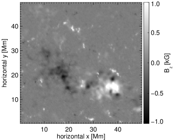
Gudiksen & Nordlund (2005a, b) used an observed magnetogram with an spatial extend of 250x250 Mm2. Because of the requested grid size, the magnetogram was scaled down by roughly a factor of 5 to fit into the computational domain. A resolution of 400 km is required to resolve both the granular motion and the temperature gradient in the transition region. This downscaling removes small-scale magnetic network patches. We use the same magnetogram as in Gudiksen & Nordlund (2005a, b) but to investigate the influence of the interaction between the active region and quiet Sun network fields small-scale features have to be introduced. The network flux is taken from a second set of observations and is enhanced by a factor of five to increase the interaction with the active region. The resulting magnetogram represents a small active region with a spatial extend of 50x50 Mm2 and is depicted in Fig. 1. To fill the computational domain with magnetic flux, we extrapolated a potential field. The resulting corona was dominated by a large-scale loop connecting the main polarities of the active region.
The initial plane-parallel temperature and density stratification match the model atmosphere by Vernazza et al. (1981). The atmosphere is at rest at the beginning.
Once the simulation is started, after some 30 min solar time, the solution is independent of the initial setup; e.g., the typical granule life time is 5 min and the Alfvèn crossing time about one minute. Since we start with a potential field, the averaged heating rate is zero at the beginning. After initialization time, the heating rate reaches values that are equal to the temporal average for the rest of the simulation time. Figure 2 shows the volume average of the squared current density beginning with the initial conditions. The dashed line in fig. 2 marks the time after which data was taken for the analysis presented in this paper. This guaranties that data taken do not depend on the initial condition. The atmosphere becomes highly structured and dynamic with high velocities, but the overall and averaged appearance remains more or less constant.

2.3 Boundary conditions
Photospheric motions at the lower boundary are the driving mechanism of the dynamics in the upper atmosphere. These motions with power spectra similar to observed velocity spectra shuffle around the foot points of magnetic field lines. This leads to non force-free magnetic fields with currents which heat the plasma by dissipation. The horizontal photospheric motions at the lower boundary are computed in a similar way as done by Gudiksen & Nordlund (2002, 2005a, 2005b). These random-like horizontal motions are time-dependent and prescribe a velocity field similar to that found in the real solar photosphere from observations. The vertical velocity at the bottom boundary, as well as all three components of the velocity vector at the top boundary, are zero at all times. The temperature and density at the bottom boundary are kept at their initial values. At the top boundary, the temperature and density have vanishing first derivatives in the vertical direction, but no specific values for or are imposed.
The initial magnetic field configuration at the lower boundary evolves in time following the induction equation. Because photospheric random motions would corrode the active region, we update the magnetic field at the lower boundary by its initial value. The time scale involved is chosen so that the time series of the computed active region looks similar to an evolution of an active region on the Sun. At the top boundary we assume a potential field.
In the horizontal directions the box is fully periodic.
2.4 Numerical setup
We use the Pencil Code (Brandenburg & Dobler 2002) to run our numerical model. It is a highly modular compressible MHD code tested on several astrophysical problems and can be used for massive parallel computing using Message Passing Interface (MPI). The numerical scheme is a finite difference scheme comprising a sixth-order spatial derivative and a third-order Runge-Kutta time-stepping scheme. The calculation is performed using 128 grid points in each direction. This is the minimum amount of grid points needed to resolve the granular motions on an 50x50 Mm2 area. The resulting grid spacing is on the order of 390 km in the horizontal and 230 km in the vertical direction, respectively.
Parameters are set to their values found in literature except the resistivity and the dynamic viscosity . Both are set to fulfill the requirement of a grid Reynolds number close to unity. The simulations runs for one solar hour before we start to collect data with a cadence of 30 seconds for another solar hour. This gives us 120 snapshots of all physical variables such as velocity, temperature, density, and magnetic field.
The model is conducted on a cluster consisting of 32 Intel CoreDuo (TM) Xeon processors. The cluster is located at the Kiepenheuer-Institut for Solar physics, Freiburg, Germany. The typical time step of the simulation is about one millisecond solar time, which results in an overall computing time on the order of 25.000 cpu hours.
3 Results
The model shows a highly dynamic and structured corona as a response to the photospheric driving imposed at the lower boundary. The total energy is balanced and the model corona reaches temperatures above one million Kelvin. Horizontally averaged temperature and density profiles (Fig. 3) show the different layers starting from the photosphere, the chromosphere, and the transition region followed by the corona. The resulting average atmosphere is similar to a Vernazza et al. (1981) standard model. The density drops by several orders of magnitude before it has a large constant scale height above 8 Mm. The average coronal density is on the order of kg m-3 or the particle number density m-3.
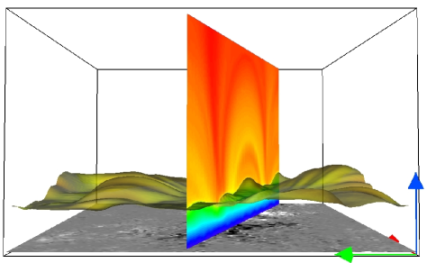
The transition region in the averaged temperature profile spans a height of 2 Mm. Figure 4 shows the isosurface at 105K above the vertical magnetic field component at the lower boundary. This highly corrugated surface represents the center of the transition region. The density along the isosurface is not constant, and therefore the emissivities of emission lines will vary. The transition region above the main polarities is at lower heights as the average transition region height. This is a result of the anisotropic heat conduction. More heat is channeled along the magnetic field lines towards the main polarities than to the network flux because the corona is mostly connected to the strong magnetic flux concentrations. Thus the transition region migrates downwards to regions of higher density. The stronger heat income is then compensated for by increased radiative loss (cf. Sect. 2).
Figure 4 shows loop like structures with dense regions separated by loops with lower density. The loops are filled and release their mass during the one-hour simulation. The picture shows only one snapshot. A temporal analysis is done in Sect. 3.3.
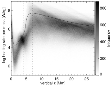
In Fig. 3 the magnetic transition region is marked at a height of 4 Mm. This height depends on the typical length scale of the magnetic features in the photosphere and is discussed in Sect. 3.1.1. The height of the maximum of the horizontally averaged heating rate per particle (cf. Sect. 3.1.2) is located at 7 Mm (Fig. 3).

3.1 Average spatial distribution of the heating rate
The average heating rate drops dramatically with height up to some 4 Mm and then falls off more slowly but still exponentially (cf. Fig. 5). Below 4 Mm most of the small-scale magnetic field lines emerging from the photosphere are closed back to the surface and thus causing the bend seen in Fig. 5, which is discussed in Sect. 3.1.1. In contrast, the average heating rate per particle peaks at some 7 Mm height (cf. Sect. 3.1.2). Overall, the average heating rate through Ohmic dissipation corresponds well with the average Poynting flux into the upper atmosphere at all heights (cf. Sect. 3.1.3).

3.1.1 The magnetic transition region
The vertical magnetic field at the lower boundary consists of two strong opposite polarities and small-scale network flux patches. Field lines emerging from the active region reach high up into the atmosphere and build the coronal loop. Field lines starting at lower flux concentrations close back earlier and thus are shorter. The top panel of Fig. 6 shows a histogram of lengths of field lines traced from the lower boundary. The 256x256 starting points are equally distributed in the x-y-plane. The number of field lines decreases in roughly inverse proportion to length. But there is a change in the distribution function at roughly 15 Mm. Below, i.e. from 0 to 15 Mm, the number of field lines per length interval decrease more slowly than exponentially. The total fraction of magnetic field lines in this interval is 75%. These field lines connect network patches and reach a height of roughly 4-5 Mm when semi-circular loops are assumed. For lengths above 15 Mm the number of field lines decreases roughly exponentially up to some 40 Mm. For even longer field lines we find a clustering with the longest field lines reaching almost the top of our domain. These field lines connect the main polarities and are less than 1% in total.
A distinct change in the distribution of field line lengths is visible in Fig. 6 at a length of about 15 Mm. This field line length corresponds to an apex height of about 4 Mm (assuming a semi-circular loop). This indicates that at heights in the computational domain below roughly 4 Mm the magnetic field topology is dominated by short loops connecting small-scale features. Above this height the volume is dominated by the longer field lines connecting the two main magnetic patches of the active region. We therefore denote this height range at about 4 Mm where the magnetic topology changes from small-scale to large-scale as the magnetic transition region. This can also be seen as a kink in the distribution of currents (or more exactly the heating rate ) with height in Fig. 5 (Sect. 4.2). This definition is similar to Jendersie & Peter (2006).

3.1.2 Foot-point dominated heating
We analyzed the heating rate for each snapshot of our model by investigating the Ohmic heating rate (cf. Eq. (3)) at all grid points. It corresponds to the volumetric heating rate and Fig. 5 shows its horizontal averages for one time step. The volumetric heating rate decreases over more than ten orders of magnitude from the photosphere to the corona.
From the photosphere to the upper chromosphere at 4 Mm, the heating rate decreases about eight orders of magnitude. Thus 99% of the energy is deposited in the chromosphere, and the chromosphere acts as an energy buffer.
Above 4 Mm (lefthand side in Fig. 5) the heating rate drops exponentially with a scale height being on average around 5 Mm. Gudiksen & Nordlund (2005b) found an average scale height of 5 Mm in their model, too. For both the transition region and the corona, the heating scale height is constant. The volumetric heating rate at the top of the chromosphere is approximately W m-3.
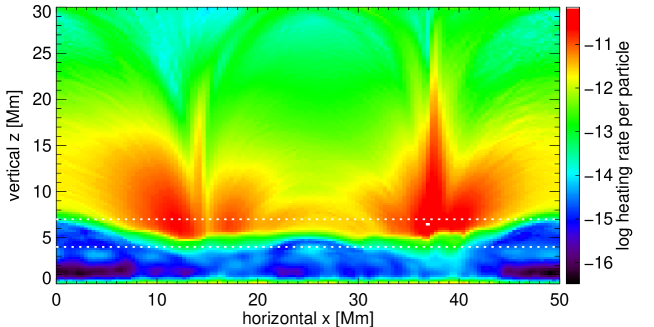
The density scale height (cf. Fig. 3) at roughly 104K (below 5 Mm) is about 0.3 Mm. Due the rapid temperature increase up to K the density scale height becomes 13 Mm above 7 Mm. Between the heights of 5 Mm and 7 Mm, the volumetric heating rate drops exponentially with a scale height between the density scales at these levels. This leads to a maximum specific heating rate per particle as illustrated in Fig. 7. The specific heating rate, i.e. per particle, increases starting at the lower chromosphere with a scale height of 0.5 Mm, whereas the specific heating rate drops exponentially with a scale height of 6 Mm above 7 Mm height. Thus, even though most of the energy is deposited in the chromosphere, the available energy per particle is higher in the corona.
The volumetric heating rate (cf. Fig. 5), as well as the heating rate per particle (cf. Fig. 7), shows that the heating of the coronal loops is foot-point dominated, and yet there is heating also in the upper part of the corona.
3.1.3 Energy flux into the atmosphere
The volumetric heating rate can be converted into an energy flux by assuming that all energy comes from the lower boundary. This is the case for the Ohmic heating as the driving occurs at the photosphere and the magnetic field dominates the upper atmosphere. The energy flux density is a function of height and gives a measure for the energy per unit time that has to pass this height through a unit plane. The value of can be derived from the volumetric heating rate by integrating from to infinity; i.e., the heating above is powered by the energy flux through the height ,
| (10) |
The horizontal average of the energy flux density is depicted in Fig. 8. The energy flux into the upper atmosphere is ranges from 106 to 107 W m-2 and decreases rapidly up to 4 Mm in height, the magnetic transition region. At the bottom of the transition region the energy flux density is a few times 100 W m-2. This is consistent with the typical observation-based estimations for the energy flux needed to heat and sustain the corona (e.g. Withbroe & Noyes 1977). The energy flux decreases further to a few times 10 W m-2 in the upper part of the corona.
The Poynting vector describes the direction and the strength of the energy flux in an electro-magnetic field. Using the induction equation (5) and Ohm’s law, we can write the Poynting vector independent of the electric field as
| (11) |
Figure 8 depicts the horizontally averaged vertical component of the Poynting vector. As the Ohmic heat is energy converted from the magnetic field, the Poynting flux roughly follows the energy flux derived from the heating rate. Because the Poynting flux depends on the plasma velocities it shows more temporal variation. Galsgaard & Nordlund (1996) found that the dissipation rate scales linear with the Poynting flux at the lower boundary. Averaging over a short time period we find that this relation is even valid for all heights. The energy released in a sub-volume corresponds to the incoming Poynting flux.

3.2 Current sheets and nanoflares
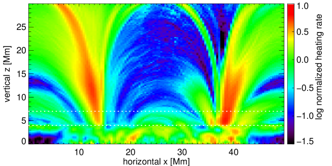
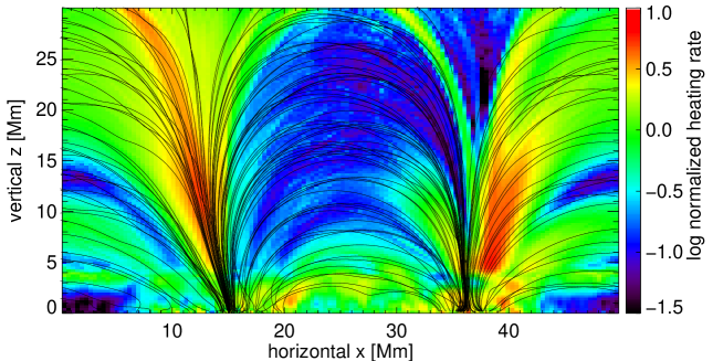
The horizontally averaged heating rate in the simulation is almost constant in time. Investigating smaller volumes, i.e. at high spatial resolution, the heating rate reveals a highly dynamic nature with a broad range of time scales. Figure 9 depicts heating rate in a slab placed above the main polarities of the magnetogram. The heating rate is normalized by its horizontal average in order to remove the steep vertical gradient (cff Fig. 5).
We used a narrow 3D volume, i.e. a slab, rather than a 2D plane and integrate over one direction. A vertical cut through the domain would only show the intersection of the magnetic field lines with the plane but not a part of the loop. Samples of field lines that fit completely into the slab are shown in Fig. 10. The field lines seem to intersect, which is only an effect of the projection onto the x-z plane.
In the coronal part the Ohmic heating rate is organized in current sheets oriented parallel to magnetic field lines. These structures exist at the resolution limit and are several grid cells wide. The alignment of the heating structures to the field lines is illustrated in Fig. 10. Below 4 Mm, the magnetic transition region, the normalized heating rate shows small structures that indicate the short field lines (cf. Sect. 3.1.1).
The normalized Ohmic heating rate in Fig. 9 only illustrates the spatial distribution of the heating but does not give any measures. The specific heating rate per particle in the same slab is depicted in Fig. 11. It also shows the concentration of the heating in structures along the magnetic field lines. Furthermore, the foot-point dominated heating is illustrated. As shown in Fig. 7 the specific heating rate peaks at around 7 Mm.
Current sheets along magnetic loops have also been investigate by e.g. Rappazzo et al. (2007) in high resolution loop simulations investigating the Parker field line tangling that leads to Ohmic dissipation. Their model compares well to our setup including constant resistivity, whereas they used a so-called hyperresistivity. But in contrast our model extends over larger volume and comprises a wide range of magnetic structures in a more realistic geometry.
3.3 Heating dynamics and response along field lines
In the previous section we showed that the volumetric heating rate is organized in current sheets. A closer look at the current sheets reveals that these current sheet are discontinuous. Furthermore, the discontinuities change in time. Therefore we analyzed the time dependence of the heating rate along magnetic field lines. Figure 12 illustrates the selected six different field lines that are traced in the complete 3D box respecting the periodicity of the domain. These field lines are selected to represent different heights and different connectivities between the main polarities, as well as into network patches. A list of properties of the selected field lines is given in Table 1. In the subsequent discussion of the physical properties, we use the word loop instead of the mathematical construct of a field line. Loop # 2 reaches the bottom of the transition region, whereas loops # 1 and 3 extends above the transition into the base of the corona. Loops # 4 to 6 extend into the corona. In comparison to half circles, the apex height of loops # 1 to 3 is smaller than half their foot-point distance, implying that these loops appear somewhat flattened. Loops # 4 to 6 are stretched out into the corona with heights exceeding half the foot-point distance.
| No | apex height | length | foot point distance |
|---|---|---|---|
| [Mm] | [Mm] | [Mm] | |
| 1 | 7.1 | 28.9 | 22.8 |
| 2 | 5.0 | 26.5 | 22.9 |
| 3 | 8.9 | 33.8 | 25.2 |
| 4 | 24.7 | 76.7 | 25.0 |
| 5 | 23.7 | 76.5 | 26.7 |
| 6 | 29.0 | 87.5 | 48.9 |
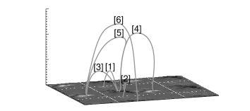
For the following investigation we did not follow the field lines in time, instead study the plasma properties in time on the trajectory defined by the field line at the beginning of the time interval under study. This is justified by the low (e.i. some km/s) velocities perpendicular to the magnetic field and the corresponding displacement over 10 minutes is close to the grid spacing.
3.3.1 Specific heating rate per particle
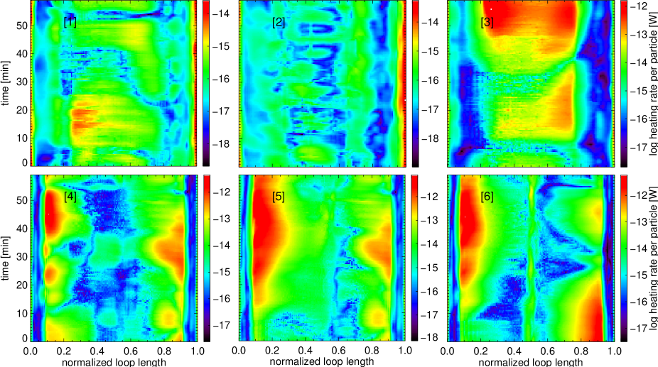
Figure 13 displays the specific heating rate per particle for one solar hour along the magnetic field lines. Different types of heating events can be found. On the left side of panels [5] and [6], the heating is continuous over more than 20 minutes. On the other hand, loop # 3 shows at the top (middle of panel [3]) short-lived heating events. Since the numerical time step is only a few milliseconds these events are resolved well in the simulation.
Loops # 1 and 2 connecting the main polarities with the network field are mainly foot point heated at photospheric levels; however, the heating of the foot points in the network (cf. righthand side of panels [1] and [2]) is stronger than the heating at the negative main polarity of active region. As the velocities are quenched at strong magnetic fields, the shear of the foot points becomes larger for the network flux patches.
Loop # 3 undergoes two main heating events at its top. The first event (from 15 min to 30 min) consists of several short small-scale events. The energy content of these small events can be computed and is similar to nanoflares, i.e. some 1017 J, so that the first event compares to nanoflare heating or heating by nanoflare storms. The second (starting at 30 min) event starts with nanoflare heating before the heating gets stronger. The entire top of loop # 3 is heated in the last couple of minutes.
Loop # 4 is heated mainly at the height of the transition region where the heating events have durations between 10 and 20 min, and they occur on both sides of the loop. Loops # 5 and 6 undergo a long heating event at their foot points (on the lefthand side of panels [5] and [6]).
As already shown in Figs. 5 and 7 loops are predominantly heated at their foot points. However, exceptions, e.g. loops # 1 or 3, can be found.
3.3.2 Temperature variation
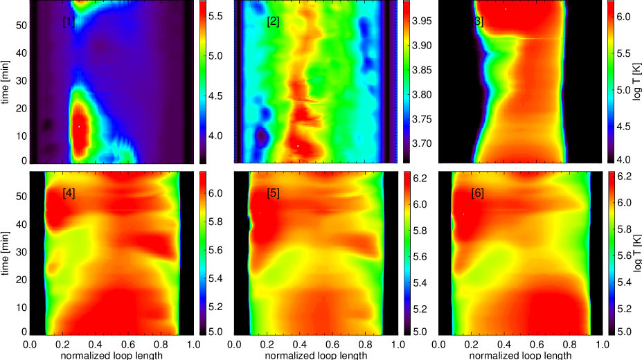
The temporal evolution of the temperature is depicted in Fig. 14. Loop # 1 partly increases in temperature by an order of a magnitude at the beginning of our time series. At this time also the specific heating rate shows a peak.
Loop # 2 is the coolest and lowest loop. Its maximum temperature at the top decreases with time, nevertheless, heating events seem to occur that are not clearly visible in panel [2] in Fig. 13. Viscous heating has to be taken into account to explain the small temperature variations of this loop. Because this loop is entirely embedded in the chromosphere, the temperature (internal energy) is also slightly influenced by the Newton cooling term (cf. Sect. 2.1).
Loop # 3 shows a nice correlation between temperature variation and the specific heating rate, but in comparison the temperature along the field line is less structured. Due to the high efficiency of the anisotropic Spitzer heat conduction, the internal energy is distributed along the field line on short time scales. Small temperature variations due to the nanoflare heating are smeared out rapidly.
Loops # 4 to 6 also illustrate a nice correlation between the specific heating rate and the temperature. At times when the foot points are not heated the loop cools down. When the heating sets in not only small regions but also the entire loop gets hotter as a result of the efficient Spitzer heat conduction. For short time periods the loops are almost isothermal.
3.3.3 Vertical velocities
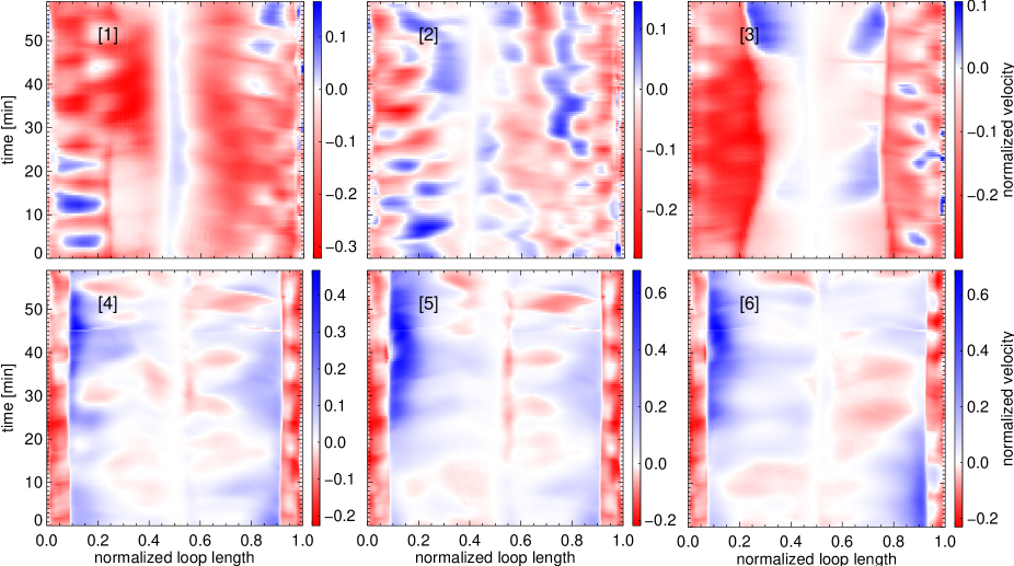
Figure 15 shows the temporal evolution of the vertical component of the plasma velocity parallel to the magnetic field lines. The velocity is divided by the local sound speed to resolve the large difference between the photospheric values of a few km s-1 and the coronal flows up to some 100 km s-1. In general, the velocities in the box are subsonic.
By normalizing one can qualitatively distinguish between the types of motions that are a response to the heating along the field line. The signature of the granular motions in the lower boundary is seen as periodic changes of up and down flows at the foot points of the field lines. These motions have a period of roughly 5 min, which corresponds to the lifetime of the granulation driving the magnetic field in the photosphere.
Loop # 1 is not heated much, and it cools down for the given time series. One effect is that the loop drains. The apex seems to move upwards, which can be understood as a motion of the field line itself. As the motion is much slower than one km s-1, field line tracing can be neglected, as argued above.
Loop # 2 shows a mix of up flow and down flow events along the loop. A clear relation cannot be found when this is compared to the specific heating rates. The chaotic like heating events result in quite irregular flow patterns.
Loops # 3 to 6 again show a nice correlation between the specific heating rate (Fig. 13) and the vertical velocities (Fig. 15). At places of strong heating the plasma evaporates and is filled into the loop. The velocities are upwardly directed (blue color) and ranges from 50 km s-1 to over 100 km s-1. At times of no heating, the coronal plasma cools down by anisotropic heat conduction and radiative losses and starts to drain (red color) out of the loop.
Loop #3 reveals a strong downflow on the lefthand side. There the loop is much denser than the opposite foot point. Thus the specific heating per particle is less and the radiative cooling is more efficient. The loop cools down quickly, and the plasma has to drain out of the loop. After some 45 min, the heating becomes strong enough so that plasma evaporation can take place again.
Loop # 6 shows a siphon flow first from the right to the left side, and after some 15 min the siphon goes from the left to the right. These siphon flows are a result of the asymmetric heating of the foot points. First the foot point on the righthand side is heated, then the one opposite it. After some 45 min, the loop is above one million degrees on both sides due to the heat conduction. The draining stops and at both sides the loop is filled with plasma.
Even though loops #4 to 6 are foot-point heated either on one or the other, a siphon flow is suppressed as soon as the loop approaches isothermal. The highly efficient Spitzer heat conduction leads to the almost constant temperatures for which the loops either are filled by plasma or they drain.
4 Discussion
Our approach of a 3D MHD numerical model successfully produces a one million degree hot corona above a small active region. The heating mechanism following Parker (1978) self-consistently produces a heating rate strong enough to balance Spitzer heat conduction and radiative loss. The empirically based photospheric motions create the dynamics of the system. The model corona is in a quasi-stationary state where energy input by the Poynting flux is balanced by radiative loss. Other 3D models also find a hot corona but use additional empirically based heating mechanisms (e.g. Abbett 2007), or else the spatial extend is less (e.g. Martínez-Sykora et al. 2009) than in the model presented in this paper. In contrast to the models of Gudiksen & Nordlund (2002, 2005a, 2005b), which are similar to ours, we also included the magnetic flux of the network patches.
4.1 Notes on the heating rate
The heating rates found in our model are sufficient to sustain a hot corona. Implemented Ohmic heating is only an approximation because the magnetic resistivity used in the simulation is much greater than one would expect for the coronal plasma following classical transport theory (e.g Spitzer 1962). The resistivity describes the process of conversion of magnetic to thermal energy, and the value used in our model is increased by about eight orders of magnitude, in order to have magnetic grid Reynolds numbers of order unity. So that the currents are actually dissipated.
The magnetic Reynolds number describes the proportion of the advective to the resistive process for a certain length scale or the proportion of the resistive time scale to the advective time scale
| (12) |
where is the rms velocity and a given length scale. If we assume coronal values for the resistivity (e.g. Spitzer 1962), then we have to look at cm length scales to obtain a Reynolds number of 1 where the currents are dissipated. These length scales are not resolved, but we must use the grid spacing to compute the magnetic grid Reynolds number. Using 400 km results in a resistive time scale several orders of magnitude larger than the advective time scale. Thus we would not dissipate any currents in the time of our simulation. This contracts observations, beacause the life time of active regions or eruptive events such as flares illustrates that the resistive process is much faster. To circumvent this dilemma we chose the resistivity such that the magnetic grid Reynolds number is on the order of unity and therefore the time scales are comparable. Naturally we find a wide spread of Reynolds numbers in our domain.
Galsgaard & Nordlund (1996) also investigated the dependency of the resistivity on the numerical resolution. For the first event in their model they found a logarithmic scaling, but for the rest the dissipation seems to be independent of resolution. Lowering the resistivity would just postpone the dissipation process. As long as the Poynting flux into the domain is constant, the dissipation rate is fixed on larger time scales. Galsgaard & Nordlund (1996) find a scaling law between the dissipation rate and the Poynting flux that only depends on the granular motions and the magnetic field in the photosphere. This justifies our choice of to have a magnetic Reynolds number of order unity.
4.2 The magnetic transition region
At a height of about 4 Mm the magnetic structure of the atmosphere is abruptly changing (Sect. 3.1.1). This manifests itself most clearly in the kink of the average heating rate and the energy flux as a function of height (Figs. 5 and 8). This is related to the height where most of the small-scale (granulation scale) magnetic flux closes, defining a magnetic transition region. Only above this height does the upper atmosphere reach a magnetic state that represents the magnetic structure of the corona.
This magnetic transition region is located above the height of the classical canopy (Giovanelli 1980; Solanki et al. 1992), which is found below 1 Mm. The latter is set by the rapid expansion of the magnetic field with height, because the gas pressure drops exponentially and a horizontal equilibrium of gas and magnetic pressure has to be achieved (e.g. Solanki & Steiner 1990). Basically the classical canopy is a magneto-hydrostatic effect.
In contrast, the height of the magnetic transition region can be understood by the potential field extrapolation of the distribution of magnetic flux at the surface. In a numerical experiment Jendersie & Peter (2006) show that, in quiet Sun regions above the network, the small-scale magnetic concentrations would produce numerous short loops reaching up to about 4 Mm (cf. their Fig. 3). The small-scale structures push up the expanding field lines from the larger magnetic patches, so in contrast to the classical canopy, where the (predominantly horizontal) magnetic field is overlying a field-free region (e.g. Steiner & Murdin 2000) a larger-scale magnetic field is found above a volume with small-scale closed magnetic field lines, in the case of the magnetic transition region .
Our current model carries this concept further by giving up the assumption that the magnetic field is potential in nature (i.e. current-free). The resulting currents found in the 3D MHD model are very strong in the photosphere and chromosphere because of the shear applied by the horizontal foot-point motions of the granular convection. The heating rate drops roughly exponentially with a very small scale height of less than 0.5 Mm. Above the magnetic transition region, where the larger scale magnetic structures dominate, the heating rate still drops exponentially (on average), but now much more slowly with a ten times greater scale height of about 5 Mm.
4.3 The chromosphere as an energy filter
While the heating is highly intermittent in time and space, the horizontally averaged heating rate is almost constant in time. At the magnetic transition region, i.e. at the top of the chromosphere, the volumetric heating rate drops to just below 10-4 W m-3. There the energy flux into the corona heating up the upper atmosphere is a bit more than 100 W m-2. This is consistent with typical estimates of the energy demands derived from observations (e.g. Withbroe & Noyes 1977), especially when considering that we describe a small active region in our model. Our results are also consistent with Gudiksen & Nordlund (2002, 2005a, 2005b).
It is most remarkable that in our 3D MHD model the upwards directed energy flux heating the corona is dropping by about six orders of magnitude (Fig. 8) from the surface to the base of the corona, i.e. the magnetic transition region. This is consistent with the real Sun, because in the model we have roughly the same Poynting flux at the surface as found on the Sun. This implies that only the 10-6th part of the energy flux at the surface makes it into the corona. Or in other words: about 99.9999% of the energy is dissipated in the lower atmosphere below the magnetic transition region! It has to be stressed that no fine-tuning was applied to the model to get the correct energy flux into the corona, i.e. to dissipate just 99.9999% (and not all) of the energy in the lower atmosphere.
Thus the lower atmosphere below the magnetic transition acts as an efficient filter for the energy transported upwards to heat the corona. It would be very interesting to investigate how the efficiency of this filter changes with the parameters of the 3D MHD model and the boundary conditions; i.e., what can be expected for other types of stars than our Sun. This could affect how we understand why the X-ray luminosity in more active stars is strongly enhanced (up to 104; Pizzolato et al. 2003), while the filling factor of the coronal plasma can be increased by a factor of only about 100 (assuming a filling factor for the Sun of about 1%). Further studies will have to elucidate this problem.
4.4 Individual strands and coronal loops
While in a 1D numerical model for a coronal loop one can afford a high spatial resolution to resolve strong gradients and shocks along the loops or include ionization processes, a 3D MHD model provides the possibility of investigating how neighboring structures interact and getting a better (more self-consistent) description of the heating rate. Therefore it is interesting to compare our 3D model to state-of-the-art 1D loop models, as well as to multi-stranded loop models.
4.4.1 Thermal and dynamic response of individual loops
If we investigate individual field lines in our 3D computational box, we can follow the temporal evolution of the physical parameters in the same manner as in 1D models for coronal loops (Sect. 3.3, Figs. 13 to 15). This shows a thermal and dynamic evolution of the loops, i.e. variations in temperature and velocity, on time scales from well below minutes to one hour.
While the time scale of the driver in the photosphere is only several minutes (granulation), the response of the corona in terms of the heating rate shows much faster variations. This is a consequence of the non linearity of the physical process of field line braiding and energy conversion. Therefore the rapid variations in temperature and velocity seen in the coronal parts of individual loops are not a signature of the photospheric driving, but the response of the plasma to the small heating events in rapid succession. In that sense the dynamics of the corona is decoupled from the photosphere. (In the lowermost parts of the loops a clear signal of the photospheric driver can be seen, of course, cf. Fig. 15).
The variations on longer time scales are (partly) due to the long-term evolution of the larger magnetic field patches in the photosphere. For example, over a half hour the granular motions can create (or destroy) by chance larger patches of stronger magnetic field, which in turn result in an increased heating of the overlying corona (e.g. loops #5 and #6 in Fig. 13). In general the evolution of the temperature of a loop on these longer time scales roughly follows the heat input from below, but with some modification because of the long cooling time of the coronal plasma.
In general the dynamic evolution as found along field lines in our 3D models compares well with state-of-the-art 1D loop models. For example, we find dynamic processes such as cooling, draining, or siphon flows of the same order of magnitude as comparable gradients as described, e.g., in Müller et al. (2003, 2004). While they assumed an exponential drop of the heating rate in their loops with a comparable scale height, they kept the heating constant in time. In the light of our finding that the details of the photospheric driver (on short time scales) are not important for the coronal dynamics, this can be considered as a minor difference. Therefore we can conclude that our results for individual loops forming in the 3D MHD model compare well to high-resolution 1D loop models. Of course, the computational effort prevents us from including, e.g., ionization processes, but we can properly resolve the thermal and the flow structure within the loops. This allows us to also draw conclusions on multi-stranded loop structures.
4.4.2 Comparison to multi-stranded loop models
In their multi-stranded loop models Patsourakos & Klimchuk (2006) assume that a coronal loop consists of individual strands that are treated as independent 1D models. This is justified by the low heat conduction across the magnetic field, which basically isolates the individual structures. Their strands are heated by increasing the heating rate for some time (and by this mimicking nanoflares). In our 3D model a large loop, such as seen in the vertical cut of Fig. 4, contains numerous loop-like current sheets that are parallel to the magnetic field, as depicted in Figs. 9 and 10. These current sheets can be very thin, down to the size of the grid cells of the computation. Thus one could consider a bundle of field lines with the parallel current sheets (Fig. 10) as the many strands making up a loop in the multi-strand model.
However, there is a major difference to the multi-strand model. While the cross-field conduction is very low, i.e. the strands are thermally isolated, the 3D model incorporates interaction of the strands: the braiding of the magnetic field lines causes the loop-shaped current sheets parallel to the magnetic field. This results in a self-consistent impulsive heating of the individual strands, whereas Patsourakos & Klimchuk (2006) release the nanoflare energy ad hoc. Recently López Fuentes & Klimchuk (2010) have employed a multi-strand model that mimics this process. They assume that the strands are displaced by photospheric motions, which sets the time for the energy release for a given strand according to Parker (1988), but there is still no interaction between the stands as these are described by 1D models.
Another difference to Patsourakos & Klimchuk (2006) is that they assume the heating is distributed uniformly along the loop, while our model gives a heating rate that drops exponentially with height. However, as the Patsourakos & Klimchuk (2006) model loops are much larger than those fitting in our computational box, it remains to be seen if this difference is significant or if this is more a property of smaller than of larger ones.
More analysis of the distribution of the heating rate in space and time as found in our 3D MHD model will have to show how this compares in detail with the assumptions of the multi-stranded loop model, and might provide important constraints for the further development of the multi-stranded loop models.
5 Conclusion
Our 3D numerical model of the solar corona successfully describes how to sustain a hot corona by the heating mechanism based on Ohmic dissipation. The average heating rate and the derived energy flux compare well to the observational requirements (e.g. Withbroe & Noyes 1977). Furthermore, the model resolves the intermittent and transient character of the heating on a wide range of energy scales.
The heating rate per particle (or mass) is found to be strongest in the transition region from the chromosphere to the corona. This is because of the scale height of the (on average) exponentially dropping volumetric heating rate is between the pressure scale heights of the chromosphere and of the corona.
The heating is concentrated in current sheets that are roughly aligned with the magnetic field lines and which are highly intermittent in time and space. In general this supports the idea that the corona is heated by a large number of small energy depositions, often named nanoflares (e.g. Parker 1988).
The dynamics within a corona loop (or a strand thereof), i.e. single field lines in the complex 3D magnetic field, follow the transient heating events. Loops with siphon flows, as well as irregular flow patterns, can be found in the 3D MHD model. The time-dependent heating rate along individual field lines as found in our 3D MHD models may be used as input to higher resolution 1D loop models including, e.g., non-equilibrium ionization.
The results show that 3D numerical box models of the corona are a useful tool to investigate the nature of coronal heating, in particular the distribution of the heating rate in time and space. The transient heating can be investigated down to energies well below energetic events currently observed on the Sun.
Acknowledgements.
We would like to thank Wolfgang Dobler for introducing us to the Pencil Code. Special thanks are due to Boris Gudiksen for the discussions when we started this project and for providing the code for the photospheric driver that we used in earlier experiments. This work was supported through grants by the Deutsche Forschungsgemeinschaft (DFG).References
- Abbett (2007) Abbett, W. P. 2007, ApJ, 665, 1469
- Aiouaz et al. (2005) Aiouaz, T., Peter, H., & Keppens, R. 2005, A&A, 442, L35
- Boyd & Sanderson (2003) Boyd, T. J. M. & Sanderson, J. J. 2003, The Physics of Plasmas (Cambridge University Press)
- Bradshaw & Mason (2003a) Bradshaw, S. & Mason, H. 2003a, A&A, 407, 1127
- Bradshaw & Mason (2003b) Bradshaw, S. & Mason, H. 2003b, A&A, 401, 699
- Brandenburg & Dobler (2002) Brandenburg, A. & Dobler, W. 2002, Computer Physics Communications, 147, 471
- Cook et al. (1989) Cook, J. W., Cheng, C.-C., Jacobs, V. L., & Antiochos, S. K. 1989, ApJ, 338, 1176
- Galsgaard & Nordlund (1996) Galsgaard, K. & Nordlund, Å. 1996, J. Geophys. Res., 101, 13445
- Giovanelli (1980) Giovanelli, R. G. 1980, Sol. Phys., 68, 49
- Gudiksen & Nordlund (2002) Gudiksen, B. & Nordlund, Å. 2002, ApJ, 572, L113
- Gudiksen & Nordlund (2005a) Gudiksen, B. & Nordlund, Å. 2005a, ApJ, 618, 1020
- Gudiksen & Nordlund (2005b) Gudiksen, B. & Nordlund, Å. 2005b, ApJ, 618, 1031
- Hansteen (1993) Hansteen, V. H. 1993, ApJ, 402, 741
- Jendersie & Peter (2006) Jendersie, S. & Peter, H. 2006, A&A, 460, 901
- López Fuentes & Klimchuk (2010) López Fuentes, M. C. & Klimchuk, J. A. 2010, ApJ, 719, 591
- Martínez-Sykora et al. (2009) Martínez-Sykora, J., Hansteen, V., DePontieu, B., & Carlsson, M. 2009, ApJ, 701, 1569
- Mok et al. (2010) Mok, Y., Lionello, R., Mikic, Z., & Linker, J. 2010, in American Astronomical Society Meeting Abstracts, Vol. 216, American Astronomical Society Meeting Abstracts #216, #300.03–+
- Müller et al. (2003) Müller, D., Hansteen, V. H., & Peter, H. 2003, A&A, 411, 605
- Müller et al. (2004) Müller, D., Peter, H., & Hansteen, V. H. 2004, A&A, 424, 289
- Parker (1978) Parker, E. N. 1978, ApJ, 221, 368
- Parker (1983) Parker, E. N. 1983, ApJ, 264, 642
- Parker (1988) Parker, E. N. 1988, ApJ, 330, 474
- Patsourakos & Klimchuk (2006) Patsourakos, S. & Klimchuk, J. A. 2006, ApJ, 647, 1452
- Peter et al. (2004) Peter, H., Gudiksen, B., & Nordlund, Å. 2004, ApJ, 617, L85
- Peter et al. (2006) Peter, H., Gudiksen, B., & Nordlund, Å. 2006, ApJ, 638, 1086
- Pizzolato et al. (2003) Pizzolato, N., Maggio, A., Micela, G., Sciortino, S., & Ventura, P. 2003, A&A, 397, 147
- Rappazzo et al. (2007) Rappazzo, Velli, Einaudi, & Dahlburg. 2007, ApJ, 657, L47
- Rosner et al. (1978) Rosner, R., Tucker, W. H., & Vaiana, G. S. 1978, ApJ, 220, 643
- Schrijver et al. (2004) Schrijver, C., Sandman, A. W., Aschwanden, M. J., & DeRosa, M. L. 2004, ApJ, 615, 512
- Solanki et al. (1992) Solanki, S. K., Rueedi, I., & Livingston, W. 1992, A&A, 263, 339
- Solanki & Steiner (1990) Solanki, S. K. & Steiner, O. 1990, A&A, 234, 519
- Spitzer (1962) Spitzer, L. 1962, Physics of fully ionized gases (Interscience, New York (2nd edition))
- Spitzer & Härm (1953) Spitzer, L. & Härm, R. 1953, Phys. Rev., 89, 977
- Steiner & Murdin (2000) Steiner, O. & Murdin, P. 2000, in Encyclopedia of Astronomy and Astrophysics, ed. Murdin, P. (Grove’s Dictionaries)
- Ulmschneider et al. (1991) Ulmschneider, P., Priest, E. R., & Rosner, R., eds. 1991, Mechanisms of chromospheric and coronal heating (Springer-Verlag, Berlin)
- Vernazza et al. (1981) Vernazza, J. E., Avrett, E. H., & Loeser, R. 1981, ApJS, 45, 635
- Warren et al. (2010) Warren, H. P., Kim, D. M., DeGiorgi, A. M., & Ugarte-Urra, I. 2010, ApJ, 713, 1095
- Withbroe & Noyes (1977) Withbroe, G. L. & Noyes, R. W. 1977, ARA&A, 15, 363