Multi-scale initial conditions for cosmological simulations
Abstract
We discuss a new algorithm to generate multi-scale initial conditions with multiple levels of refinements for cosmological “zoom-in” simulations. The method uses an adaptive convolution of Gaussian white noise with a real space transfer function kernel together with an adaptive multi-grid Poisson solver to generate displacements and velocities following first (1LPT) or second order Lagrangian perturbation theory (2LPT). The new algorithm achieves RMS relative errors of order for displacements and velocities in the refinement region and thus improves in terms of errors by about two orders of magnitude over previous approaches. In addition, errors are localized at coarse-fine boundaries and do not suffer from Fourier-space induced interference ringing. An optional hybrid multi-grid and Fast Fourier Transform (FFT) based scheme is introduced which has identical Fourier space behaviour as traditional approaches. Using a suite of re-simulations of a galaxy cluster halo our real space based approach is found to reproduce correlation functions, density profiles, key halo properties and subhalo abundances with per cent level accuracy. Finally, we generalize our approach for two-component baryon and dark-matter simulations and demonstrate that the power spectrum evolution is in excellent agreement with linear perturbation theory. For initial baryon density fields, it is suggested to use the local Lagrangian approximation in order to generate a density field for mesh based codes that is consistent with Lagrangian perturbation theory instead of the current practice of using the Eulerian linearly scaled densities.
keywords:
cosmology: theory, large-scale structure of Universe – galaxies: formation – methods: numerical1 Introduction
Cold dark matter density perturbations drive all of cosmological structure formation (e.g. Peebles, 1982; Davis et al., 1985) in the current paradigm. Their non-linear growth is followed with numerical simulations over an enormous range of scales. From scales of hundreds of Megaparsecs (e.g. Springel et al., 2005; Pichon et al., 2010) studying cosmological large-scale structure; to several hundred kilo parsecs modeling the formation and evolution of galaxies including aspects of the interstellar medium, molecular cloud-formation and black-hole accretion processes (e.g. Di Matteo et al., 2008; Wise & Abel, 2008; Ceverino & Klypin, 2009; Bournaud et al., 2010); and even the formation of the first proto-stars formed at scales of a few solar radii (e.g. Abel et al., 2002; Yoshida et al., 2008; Turk et al., 2009) are studied in cosmic context.
The fluctuations in the standard model would extend from solar system size to giga parsec scales. No single calculation would be able to capture all these scales. One may therefore strive to carry out simulations in as large volumes as possible to study a range of representative environments for the formation of particular cosmological objects. At the same time, however, high resolution is necessary to sample the underlying gravitational potential wells. A popular way to achieve large simulation boxes with as high as possible resolution for individual objects is the so-called “zoom-in” technique (following versions of e.g. Katz et al., 1994; Navarro & White, 1994). In this technique, a small region encapsulating the formation history of the object of interest is studied with much higher resolution inside of a lower resolution representation of its larger-scale cosmic environment interacting with the object through long-range gravitational forces. The aim is to represent both the variance of the fluctuations on scales of the object (sample variance) due to the use of a large volume which provides a fair sample of cosmic environments (cf. eg. Crain et al., 2009; Hahn et al., 2010), as well as the smaller scale fluctuations affecting the structure of the object directly.
Typically, two approaches have been followed for initial conditions of “zoom-in simulations”. Either, initial conditions are generated on a uniform grid at the full resolution (which can amount to a huge need for computational resources for deeply nested grids, see e.g. Prunet et al., 2008; Stadel et al., 2009) and subsequently degraded by either averaging over regions of particles, where is the de-refinement factor outside the high resolution region, or by Fourier resampling. There are several disadvantages with this approach: First, the computational requirements are immense compared to the solution sought; and second, the simple averaged velocity fields are neither continuous nor differentiable across coarse-fine boundaries, leading to spurious shocks in baryonic simulations. Alternatively, e.g. the Grafic-2 code (Bertschinger, 2001) is used which employs discrete Fourier transforms to add small scales perturbations to coarser perturbations. The Grafic-2 approach however requires the use of an anti-aliasing filter which damps out small-scale power and shows oscillatory errors at the few per-cent level that result from the combination of discrete Fourier transforms of different resolution. Furthermore, it does not incorporate the sampling of the real-space transfer function advocated by Pen (1997) and Sirko (2005). This latter aspect is a feature of all codes that generate initial conditions by an inverse Fourier transform of a sampled power spectrum on a three-dimensional lattice and thus also plagues most applications of the previous approach. Sirko (2005) has shown conclusively that this conventional method can lead to a significant error in the real-space statistical properties, in particular for small cosmological box sizes.
This paper extends on previous work by proposing a new algorithm to generate multi-scale nested initial conditions (as Bertschinger, 2001), but using a real-space convolution kernel to represent the Fourier space transfer function of density perturbations (cf. Salmon, 1996; Pen, 1997; Sirko, 2005) in a multi-scale convolution algorithm combined with an adaptive multi-grid algorithm to determine initial velocities, particle positions and densities compatible with Lagrangian cosmological perturbation theory up to second order. More specifically, the approach uses mass conservation constraints to determine the convolution kernel from an accurate real space representation of the transfer function kernel on a hierarchy of levels, which are used in FFT convolutions to obtain the density field from a hierarchical white noise field, and a two-way interface multigrid Poisson solver that achieves smooth gradients across coarse-fine boundaries. The resulting errors are confined to the boundaries and at the level of a few in units of the standard deviation of the respective fields for the interior of the refined region.
We furthermore show that using a hybrid Poisson solver (using multi-grid for the hierarchy of grids and FFT for the finest grid), our method produces particle distributions that closely match the input power spectrum also on the smallest scales and make our approach attractive also for uni-grid simulations. All the methods discussed in this paper are implemented in the initial conditions code Music (MUlti-Scale Initial Conditions). The code also includes an implementation of a linearized Boltzmann solver based on Linger (Ma & Bertschinger, 1995) that allows the calculation of cosmological density and velocity perturbations for dark matter and baryons.
The paper is organised as follows. In Section 2, we discuss a multi-scale convolution method that produces a nested density field that is consistent with both the input correlation function and the input power spectrum, and which is then used as the source field for Lagrangian perturbation theory. Computing displacement and velocity fields in Lagrangian perturbation theory (LPT) requires a numerical solution to Poisson’s equation. In Section 3, after briefly summarizing LPT, we describe the adaptive multi-grid algorithm that we use to obtain displacement and velocity fields. We also introduce a hybrid Fourier-space/multi-grid based Poisson solver which has better Fourier-space properties on small scales compared to the pure multi-grid algorithm. In Section 4, we discuss the performance of our method compared to initial conditions generated purely in Fourier-space both in unigrid and nested grid set-ups. We generalize our approach to initial conditions for two-component dark-matter and baryon simulations in Section 5 and propose the usage of the local Lagrangian approximation to generate inital baryon density fields for grid codes before we summarize and conclude our results in Section 6.
2 Generating density perturbations
In this section, we summarize methods to generate Gaussian random fields that follow a prescribed power spectrum and act as source terms for density and velocity perturbations in Lagrangian perturbation theory. We give particular attention to a convolution kernel based approach which has favourable properties in a multi-scale nested grid set-up.
2.1 Computing the seed density field
Consider an over-density field that is completely described by its power spectrum , where the tilde denotes the transformed function of a Fourier transform pair. The amplitude of density fluctuations is usually expressed in terms of the transfer function , which is defined such that
| (1) |
where is the (constant) power spectrum spectral index after inflation, and is a normalization constant. The first step in setting up initial conditions for cosmological simulations thus consists in generating a white noise sample of random values (typically sampled from a Gaussian distribution with zero mean and unit variance) and to require that their amplitudes follow a specific power spectrum . This can be achieved by multiplying the Fourier transformed white noise field with the square root of the power spectrum, i.e. for all representable on a grid of given resolution set
| (2) |
The real space over-density field is then obtained by inverse Fourier transformation, and we call this procedure “-space sampling”.
It is interesting to note that a product in Fourier space simply corresponds to a convolution in real space (cf. also Efstathiou et al., 1985; Salmon, 1996), i.e. equation (2) is equivalent to
| (3) |
where is the real-space counterpart of , and “” denotes a convolution.
It is thus mathematically equivalent whether equation (2) is evaluated in Fourier space, followed by an inverse transform, or whether equation (3) is evaluated using an inverse transform of followed by the convolution. Most cosmological initial conditions generators follow the first approach (e.g. Bertschinger, 2001), while e.g. Salmon (1996), Pen (1997) and Sirko (2005) use the second or variations thereof. The discrete realizations of the density fields derived with the two approaches will have significant differences. In particular, employing eq. (2) forces periodicity of the real space transfer function on box scales that leads to an underestimation of the two-point correlation function (see Section 2.2, and e.g. Pen 1997 and Sirko 2005 for a detailed discussion). This is particularly relevant for small cosmological boxes (), where the periodic contribution is non-negligible.
The convolution kernel can be thought of as a “propagator” of a single Gaussian white noise fluctuation at location , where is the Dirac -function. The time evolution of each single such perturbation is given by the time evolution of . Instead of a variation of the traditional method of sampling Fourier modes according to a given power spectrum, this real-space picture has thus an intuitive physical motivation: The convolution operation imprints the density perturbations due to the white noise onto space. Apart from the better behaviour of the two-point correlation function, we follow the convolution approach since it allows for an easier treatment of nested grids that are separated by sharp boundaries in real space. To achieve this, a method will be developed that correctly overlaps the “propagator” with such coarse-fine boundaries. We give an account of how we numerically compute eq. (3) in the next section and of the multi-scale convolution approach for nested grids in Section 3.
2.2 The real-space transfer function
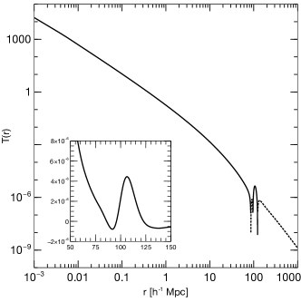
Since the transfer function is typically computed numerically using a spectral Boltzmann solver – e.g. the Boltzmann solver included with our code, Linger (Ma & Bertschinger, 1995), CMBfast (Seljak & Zaldarriaga, 1996) or Camb111Camb, written by A. Lewis and A. Challinor, can be obtained from http://camb.info, or taken from a fitting formula (e.g. Eisenstein & Hu 1998) – its Fourier transform is not available a priori. Thus, in the approach we follow, an accurate real-space transfer function is first calculated which is subsequently applied as a convolution kernel to the Gaussian white noise field using FFT convolution. Assuming a spherically symmetric transfer function , one has
| (4) | |||||
| (5) |
This real space transfer function, , can be computed using the FFTlog algorithm (Talman, 1978; Hamilton, 2000) from an input k-space transfer function . FFTlog uses the fact that the Fourier transform of a log-log function can be written as a Hankel transform which can be carried out by FFT. The resulting transform is highly accurate over many orders of magnitude. We kindly refer the reader to Hamilton (2000) for details. The component needs to be computed separately. It is obtained by a three dimensional numerical integration over the range of Fourier modes included in the simulation. This component sets the white noise level of the density perturbations.
Figure 1, shows the result of the transform from tabulated k-space transfer functions at for matter density perturbations generated with a 1D linear Boltzmann solver (cf. Ma & Bertschinger, 1995).
Finally, the convolution in eq. (3) has to be computed numerically. To this end, we compute a discretisation , with , over the entire simulation volume of length . Next, a white noise random field is created on the same discretisation. Then both and are transformed by FFT, multiplied element-by-element with one another and the result is inverse transformed to yield . Note that when sampling on a finite grid, the real-space sampled transfer function is no longer spherically symmetric when transformed by FFT to three dimensional Fourier space. However, equivalently, the traditional -space sampled transfer function is not spherically symmetric in real space.
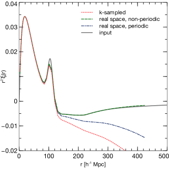
The analysis performed in this paper uses a real-space transfer function periodically replicated on the box length. This abandons the favourable properties of a truncated correlation kernel discussed in detail by Sirko (2005). However, this choice allows comparison with the classical approach that samples the k-space transfer function. For actual applications it is recommended that the truncated transfer functions should be used (which is a simple parameter in our code).
In Figure 2, we show the auto-correlation function of the transfer function kernels (equivalent to the two-point correlation function). As demonstrated by Sirko (2005), the non-periodic real space kernel perfectly reproduces the input two-point correlation function. The periodic correlator, for which we have not subtracted the mean in this case, underestimates the correlation function at large radii and the -space sampled kernel shows an even stronger drop at large radii. Note that the big drop in the -space sampled correlation function is somewhat spurious. It is partly from the periodic component, as the periodic real space kernel shows a similar suppression. However, it is mainly due to an additional integral constraint. For the -space sampled kernel, , so that
| (6) |
where is the simulation volume and the latter equality holds in the case of a spherically symmetric correlation function and amounts to the usual integral constraint on the two-point correlation function. This integral constraint however holds for a finite in the traditional -space sampling approach (while in our case) and the correlation function is thus offset by an additive constant which is equal to the integral over the correlation function outside the simulation volume. This additive constant leads to the additional deviation seen between the -space sampled correlation function and the periodic real-space equivalent which is simply amplified by the multiplication with . Any box with zero mean overdensity will therefore fulfill the integral constraint over the box instead of over an infinite volume leading to a similar discrepancy. Boxes with a non-zero mean overdensity would circumvent this problem and the difference in mean overdensity can be incorporated in a change to different effective cosmological parameters. We will not investigate further the possibility of simulations with non-vanishing mean overdensity but kindly refer the reader to Sirko (2005) for a detailed discussion of this possibility.
2.3 Generating a nested initial density field
In order to generate an accurate multi-scale representation of an initial density field, we will now describe our algorithm to perform the convolution in eq. (3) on nested grids. Particular care is taken to achieve mass conservation, as violations would affect the entire domain when the density field is used to source the displacement and velocity fields (cf. Section 3). As in the Grafic2 approach(Bertschinger, 2001), this amounts to linear constraints between the levels. However, unlike Grafic2, these constraints are not only top-down (i.e. the coarse level provides constraints for the fine), but partially bottom-up to achieve a more conservative algorithm and high-resolution sampling of the real-space convolution kernel.
2.3.1 White noise refinement
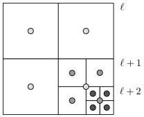
In order to generate initial conditions for a nested subdomain on the volume subdivision grid structure used in our approach (Figure 3), the white noise for the subgrid has to be consistent with that of the coarse grid. Two separate approaches can be followed that are locally mass-conserving (in the sense that the children cells average to the parent cell locally rather than that only the total mass in the subgrid domain is conserved):
The first approach uses the Hofmann-Ribak algorithm (Hoffman & Ribak, 1991). First an unconstrained white noise field is generated for level which has 8 times the variance of the noise field for level in the case of a refinement factor of 2. Next, for each group of eight children cells on the fine grid, the mean is replaced by the respective value of the noise field on the coarser level (cf. also Pen, 1997; Bertschinger, 2001).
Since this approach does not retain the Fourier modes present on the coarse grid, another approach can be devised that achieves this: (1) again, an unconstrained white noise field is generated for level at 8 times the coarse level variance. (2) In order to preserve Fourier modes that are present in the coarse grid , an FFT of both the fine grid and that part of the coarse grid that overlaps the fine grid is performed. Then all modes up to the Nyquist wave number of the coarse grid are replaced with the respective Fourier coefficients from the coarse grid, followed by an inverse transform. (3) In order to ensure conservation of mass, the Hoffman-Ribak algorithm is applied in reverse, i.e. the coarse grid white noise values are replaced by the average over the eight children of a coarse cell inside the refinement region. Since the Fourier interpolation conserves the mass of the entire subgrid, as does the averaging over children, the global mass in the simulation domain is also conserved.
Further levels can be computed by repeating first step (2) for all levels at increasing resolution, followed by the correction step that replaces all coarse cells at all coarser levels with the average over the eight fine cells, starting at the finest level. Thus, the Hoffman-Ribak constraint is fulfilled while at the same time Fourier modes are preserved between grids.
In the following, we will describe how the convolution with the real-space transfer function, eq. (3), is performed when a refinement region is present.
2.3.2 Generating convolution kernels
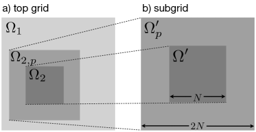
In Figure 4, we show schematically the set-up for one additional refinement level. The top grid domain consists of the domain covered by a refinement grid and the non-refined part . The refinement region at twice the resolution is given by . represents the padding around to twice the length per dimension that is needed to perform isolated Fourier convolutions.
The next step in our method is to generate convolution kernels for all required levels. In contrast to the Grafic2-approach, we construct these kernels purely in real space, starting from the finest level. For the finest level , this consists of a simple evaluation of the real-space transfer function on , i.e. for all with the origin placed at the centre.
As for the white noise, care has to be taken to maintain local conservation of mass. Thus, rather than sampling at coarser resolution, for the next coarser level , the already discretized part of the convolution kernel for the fine-level grid needs to be restricted to the coarser grid in a conservative way. This can be achieved by averaging the contributions due to all eight children cells when convolved with the kernel, i.e. we compute
| (7) |
for those grid points that correspond to the refined part of the grid. This provides the convolution kernel for a volume of the size of the refined region including the padding, i.e. for . The remaining cells outside that region, i.e. on are again sampled directly from the real-space transfer function: for all . This last step is in violation with strict mass conservation since eq. (7) does not hold outside the refined region. Since most of the mass of the convolution kernel is close to the centre, this approximation produces however negligible errors and avoids the substantial computational overhead of an exact evaluation of over the entire domain at the finest resolution. The procedure of averaging and newly sampling uncovered volume is repeated until the coarsest level is reached.
2.3.3 Noise convolution: The first refinement level
The density field on the top grid level is determined as in the unigrid case by computing on with periodic boundary conditions automatically satisfied by the FFT. For the refined region, several contributions will be co-added:
-
1.
The coarse grid contribution to the refinement region is computed by zeroing on to obtain , computing the convolution and interpolating from to . We use tri-cubic interpolation for this purpose.
-
2.
On level isolated boundary conditions apply, so has to be padded to twice its size so that an FFT-based convolution is still possible. In order to find the density due to the sub-grid alone, on is set to zero to obtain , followed by computing the convolution .
-
3.
In order to reduce errors at the boundary, a correction term is added that accounts for the fluctuations just outside . To this end, the coarse grid value of the white noise field is subtracted from each of the 8 children cells, equivalent to “unapplying” the Hoffman-Ribak method. We then zero the result of this operation on , so that it is non-zero only on and obtain . Since boundary conditions are isolated, it would be necessary to truncate the transfer function in order to have a non-periodic unconstrained white noise field. We however found that a truncation introduces larger errors than assuming periodicity (on scales larger than the subgrid). Finally, the FFT-convolution is evaluated.
-
4.
Finally, the result of the previous step is restricted also to the coarse grid, i.e. onto , in order to include information about fluctuations on smaller scales.
Finally, all three contributions are added to find the refined density field
| (8) |
on . In order to further reduce errors due to the boundary, we allow for optional additional padding of the subregion with a few grid cells and cut out the desired region at the end.
2.3.4 Noise convolution: Further refinement levels
For further refinement levels, the same steps 1-4 from above are repeated at level , , with the only difference being that the coarse grid contribution is computed using isolated boundary conditions on , i.e. with a zero padded random field . Furthermore, all coarse contributions have to be interpolated down to this level. Let be the interpolation operator, then
| (9) |
where indicates a successive interpolation between levels. We use a conservative tri-cubic interpolation for this purpose, i.e. we first perform a normal tri-cubic interpolation and then correct the eight children cells with an additive constant to ensure that their average equals the coarse cell value.
3 Initial particle positions and velocity fields
In this Section, we briefly summarize the application of first and second order Lagrangian perturbation theory to obtain the initial displacement and velocity fields which are based on solutions of Poisson’s equation. For details, we kindly refer the reader to the wide field of existing literature on Lagrangian perturbation theory (e.g. Buchert et al., 1994; Bouchet et al., 1995; Scoccimarro, 1998; Bernardeau et al., 2002). We then summarize the multi-grid algorithm which solves Poisson’s equation numerically before we discuss its extension to the adaptive multi-grid algorithm which provides solutions to Poisson’s equation on nested grids. Finally, we examine several methods to obtain velocity and displacement fields that have the same behaviour at large wave numbers as those obtained with the traditional -space sampling.
3.1 Lagrangian perturbation theory
3.1.1 First order perturbations
Lagrangian perturbation theory describes the evolution of density perturbations in the rest-frame of the fluid. The position of a fluid element at time with respect to its initial position , and the respective fluid velocity, can then be written as
| (10) |
where we call the “displacement field” which is derived using perturbation theory.
It can be easily shown that at first order in the perturbations (cf. Zel’Dovich, 1970), the displacement field can be written as the gradient of a potential which is proportional to the gravitational potential ,
| (11) |
where is the Hubble constant, is the expansion factor at time , is the growth factor of linear density perturbations (i.e. the time evolution of the growing mode) and is the gravitational potential obeying Poisson’s equation
| (12) |
Since the velocities are given by the gradient of a potential, velocities are irrotational, i.e. , in this approximation.
Note that the Gaussian over-density field is the source field of the displacements. It is not the density field that is measured after displacing the fluid elements, which is non-Gaussian. We give a derivation of the latter in Section 5.3. The Gaussian field should not be used to impose an initial density field for the baryonic component.
In order to obtain the displacement vectors from the initial over-density field , Poisson’s equation has to be solved numerically. The most common approaches use an FFT based Poisson solver (e.g. Bertschinger, 2001), while we chose a multi-grid based Poisson solver as it can be easily extended to an adaptive multi-grid solver which is able to handle nested adaptive grids in a very natural way.
3.1.2 Second order perturbations
Several studies have shown (see e.g. Munshi et al., 1994; Scoccimarro, 1998; Crocce et al., 2006; Tatekawa & Mizuno, 2007) that first order Lagrangian perturbation theory (cf. Section 3.1.1) might not be accurate enough for current simulations as it leads to e.g. significantly underestimated higher order moments of the density probability distribution functions at early times. In particular, Munshi et al. (1994) have shown that 2LPT matches the skewness of the density field for top hat collapse, while 3LPT would in addition also match the kurtosis, and so on. At second order, the displacement field contains not only contributions from the gravitational potential, but also from a second-order potential that is sourced by the off-trace components of the deformation tensor, i.e.
| (13) |
where obeys the Poisson equation , with
| (14) |
and is the growth factor of linear perturbations, and . Adding second order perturbation theory is thus algorithmically identical to repeating the steps for first order displacements: After computing the source-field using finite differences, Poisson’s equation can be solved numerically using the (adaptive) multi-grid scheme. A similar adaptive approach to generate initial conditions at second order has been made by Jenkins (2010) who use a tree-PM method to evaluate the second order contribution. Note that while our method allows for 2LPT, we only use 1LPT in this paper to aid the comparison with the typical practice in the field.
3.2 Multi-grid solution of Poisson’s equation
| Order | Laplacian | Gradient |
|---|---|---|
| exact: | ||
| : | ||
| : | ||
| : | ||
| exact: | ||
| : | ||
| : | ||
| : |
Both first and second order Lagrangian perturbation theory for velocity and displacement fields require the numerical solution of Poisson’s equation followed by calculating gradients. This can be achieved by use of the multi-grid algorithm (e.g. Fedorenko, 1961; Brandt, 1973). In order to solve Poisson’s equation
| (15) |
with periodic boundary conditions in our case, we cover with a hierarchy of grids of respective grid spacing , where , i.e. a refinement factor of 2 between multi-grid levels (cf. also Figure 3).
Define as the restriction and as the injection operator. We use the Full Approximation Scheme (FAS – Brandt, 1977), see also Trottenberg et al. (2001), to solve the discrete form of equation (15) on grid given by
| (16) |
where is a finite difference approximation to the Laplacian (as in Table 1) and is an approximation to on grid . The residual can then be written as . FAS then uses these residuals to correct the solution on level , so that (note that operators do not commute)
| (17) |
is obtained. This is equivalent to solving
| (18) |
on level , where
| (19) |
The grid at level thus provides additional source terms to the equation at level in addition to the restricted source accounting for the non-commutative nature of the operators – eq. (19) is just the commutator of the Laplacian and the restriction operator.
Within each level, corrections are propagated using a smoothing (or diffusion) scheme , typically a Gauss-Seidel sweep.
The complete FAS multi-grid scheme then consists of the following algorithm to solve , starting with :
-
1.
If , set .
-
2.
Apply smoothing steps, ,
-
3.
Calculate the residual,
-
4.
Restrict the residual,
-
5.
Restrict the smoothed solution,
-
6.
Apply the -correction,
-
7.
Apply FAS scheme recursively to solve
-
8.
Correct the solution
-
9.
Apply smoothing steps, ,
The first step ensures that the mean of the potential vanishes and that the algorithm converges in the case of periodic boundary conditions. For non-periodic boundary conditions, a direct solution would need to be computed. Throughout each cycle we enforce periodic boundary conditions, whenever is changed. The scheme is to be repeated until the norm of the residual, computed after step 9, falls below some desired threshold. Since we only call FAS once in step 7, our approach uses only V-cycles.
We found excellent convergence, i.e. a reduction of the residual by at least one order of magnitude per iteration, for all finite difference approximations of the Laplacian that we tested (up to sixth order, cf. Table 1) using the red-black Gauss-Seidel method as the smoothing operation with sweeps, simple averaging over the 8 child cells of one coarse cell as the restriction operation and straight injection of the coarse cell value into the 8 child cells as the prolongation operation .
The FAS scheme has been adopted as it operates on the solution itself on each level, while the standard multigrid operates on residuals. This allows us to incorporate conservative boundary conditions at coarse-fine boundaries more easily (cf. Section 3.3).
| Order | Flux operator |
|---|---|
| : | |
| : | |
| : |
3.3 Adaptive multi-grid
We will now describe the extension of the FAS multi-grid algorithm described above to additional nested adaptive grids, , covering non-coextensive subdomains , with . In our case, the are simply rectangular grids. Two modifications have to be made: First, restriction and prolongation only operate on overlapping regions of the domains. The remainder is treated as if it resided at the finest level. Second, Poisson’s equation on additional sub-grids is solved with the coarse grid solution acting as a boundary condition for the finer level Poisson equation . The boundary condition is realised by adding ghost zones to the sub-grids to which boundary values are interpolated.
For these coarse-fine boundaries, we first use polynomial interpolation using only coarse grid information parallel to the fine grid surface. Using these intermediate values together with values inside the fine grid, another polynomial interpolation step is performed normal to the fine grid surface (similar to Martin & Cartwright, 1996). The order of the interpolating polynomial is chosen identical to the order of the finite difference scheme for the Laplacian. This serves as a “guess” for the solution on the boundary and is thus a weak Dirichlet boundary condition. “Weak” as we will not actually use the boundary cell solution as the boundary condition.
In a second step, we apply additional constraints to the interpolated ghost zone values so that the coarse flux matches the fine flux across the coarse-fine boundary. This procedure can be easily understood by rewriting Poisson’s equation in the following way:
| (20) |
can be integrated over one grid cell (in one dimension for notational simplicity) to yield
| (21) |
where is the mass contained in cell , and is the potential flux. Applying the divergence theorem, we find that
| (22) |
i.e. the mass in cell generates a flux through the cell surfaces given by . In order for the adaptive multi-grid scheme to be conservative, the flux across common surfaces has to be identical (since the mass contained in a coarse cell is taken to be identical to the mass inside its eight children). This is trivially fulfilled for inner cells but care has to be taken at outer coarse-fine boundaries.
The flux operators are matched to the order of the Laplacian and given in Table 2. They are gradient operators of order on the cell boundaries. When convolved with the first order gradient, (which corresponds to a determination of the net flux), the respective Laplacian operator of order is recovered. Using the flux operator, the 4 fluxes due to the fine grid can be evaluated and then subtracted from the coarse flux through the same surface element. This flux difference is subtracted from the ghost zone values contributing to the fine grid flux so that the sum of the fine fluxes now matches the coarse flux. A flux-correction is necessary since otherwise the sub-grid induces artificial source terms through the ghost zone interpolation and the multi-grid algorithm does not converge (in the sense that the residual does not vanish on all levels). Note that this flux matching can be thought of as constraints on the interpolation scheme. We thus obtain mixed boundary conditions: a von Neumann boundary condition due to the flux matching, which constrains only one degree of freedom for the boundary cells at a single coarse-fine boundary, and a subordinate Dirichlet boundary condition, which constrains all degrees of freedom, but is only used to evaluate the fluxes on the fine grid (cf. also Miniati & Colella, 2007). This results in a two-way interface between coarse and fine cells. These boundary conditions ensure that gradients across coarse-fine boundaries are smooth. Note that this is not the case for the one-way interface multigrid solvers currently employed in most cosmological simulation codes due to the need for adaptive time-stepping. Using this conservative procedure we maintain multi-grid convergence (i.e. the residual reduces by at least an order of magnitude per iteration) also with an arbitrarily deep hierarchy of adaptive sub-grids.
Note that our approach to use an adaptive Poisson solver is in similar spirit as Salmon (1996) who used a tree to compute displacements and velocities, or Jenkins (2010) who also used a tree to compute the second order term for 2LPT. The advantage of the multi-grid method is however that it has a well controlled residual to the equation to be solved so that errors are easily controllable by setting the convergence criterium in terms of the residual norm rather than by tuning opening angles for the tree. The performance of a tree-based Poisson solver is particularly problematic for density fields with low constrast. Using a tree has the further disadvantage that periodic boundary conditions have to be incorporated in a hybrid way (e.g. by using FFT for the top grid). This leads to an additional source of errors arising from the long-range/short-range split.
3.4 Fourier analysis of the finite difference operators
Operating in real space requires the use of a finite difference approximation to the Laplacian “” and gradient operators “”. In Table 1, we give the standard stencil representations for the one dimensional versions of these operators. The three-dimensional versions can be obtained by subsequent convolution of the one-dimensional operators along all three Cartesian coordinate axes. In the bottom half, the Fourier transforms of the operators are given together with the exact Fourier transform of the continuous operators. Since a regularly spaced mesh is a Dirac comb, due to symmetry reasons, the Fourier transform of these operators takes the form of a cosine series, in the case of the Laplacian, and of a sine series, in the case of the Gradient. These series are approximations to the respective continuous and non-periodic transforms of the operators. The sine series representing the finite difference gradients vanish at the Nyquist wave number leading to a suppression of small scale modes. Furthermore at low order, the finite difference approximation leads to an attenuation also at slightly large scales. We will investigate the influence of this attenuation on cosmological initial conditions in what follows. We analyze non-adaptive unigrid initial conditions in this section, in order to differentiate these effects from those due to adaptive initial conditions, which will be addressed in Section 4.3.
3.4.1 Damping of small-scale perturbations
In the Zel’dovich approximation, the displacement and velocity fields are proportional to the gradient of the potential (cf. eq. 11). In this section, we investigate how the order of the finite difference approximation for the Laplacian and the gradient affects perturbations close to the Nyquist wave number , where is the grid spacing which we set equal to unity in this section for convenience.

We define as the gradient of the potential arising from a source field . The potential is solved using the multi-grid scheme outlined above, and the gradient operator is applied subsequently. The exact solution in k-space is given by , where the tilde represents the Fourier transform. Expressed by the Fourier transforms of the operators, this is simply:
| (23) |
where the last equality holds for the exact solution. We define the attenuation as the ratio between the one-dimensional finite difference solution – using approximations of a given order for and and taking their Fourier transform as in Table 1 – and the exact solution in k-space.
In Figure 5, we show this attenuation as a function of wavenumber that is to be expected from the finite difference approximations to the operators up to sixth order. All finite difference gradients have zero amplitude at so that fluctuations at this scale can not be represented in principle. A 2nd order approximation leads to significant attenuation of per cent at . However, for 6th order, attenuation is at the level of a few per cent at . We thus expect a suppression of the power spectrum at large depending on the order of the finite difference operators employed. Note that corresponds to scales of two grid cells and that the attenuation enters squared into the power spectrum.
3.5 Recovering small-scale power
Both the use of a transfer function evaluated in real space and finite difference methods lead to a loss of power at scales close to the Nyquist wavenumber. We outline methods to solve this problem in what follows. Most of these methods will lead to spectral leakage and the associated spurious oscillations (cf. 3.5.5) which poses no problem in the case of dark matter particle initial conditions but should be avoided for baryons.
3.5.1 Finite Volume Correction
As demonstrated in Section 3.3, the multi-grid method is a finite volume approach. The solution is determined by computing flux balances across grid faces. This implies that the source field is simply a cell average. Hence, implicitly, every discrete value is a piecewise constant approximation to which is incorrect in the particle case. The piecewise constant averaging is given in terms of a kernel convolution
| (24) |
In order to restore the small-scale fluctuation amplitudes, it however suffices to perform a deconvolution with the cell assignment function – equivalent to nearest grid point (NGP) assignment, see e.g. Hockney & Eastwood (1981),
| (25) |
where is the Heaviside step-function and is the grid spacing. Since has an algebraic form for its Fourier transform
| (26) |
we can perform this deconvolution in the Fourier domain and thus recover some of the sub-grid power – see also Jing (2005) who use a similar procedure for power spectrum estimation. Note that – by virtue of restoring sub-grid power – the deconvolution leads to spectral leakage. The associated ringing will however be completely filtered out by subsequent finite difference operations.
3.5.2 A hybrid Poisson solver
The attenuation of subgrid power due to the finite difference operators themselves (which however comes at the benefit of a non-oscillatory velocity field) may be considered undesirable as part of the velocity information is effectively destroyed by the finite difference approximation. Since the lack of small scale power is only relevant on the finest grid, a simple solution to circumvent this problem can be devised. Since the Fourier transforms of the finite difference operators are known, the fine grid solution can be simply replaced by the -space exact solution. Setting the right-hand side of Poisson’s equation on the boundary, we can recompute the self-gravity due to the fine grid and replace it with the one obtained with the exact -space method, i.e. using a grid zero-padded to twice its size, the correction is
| (27) |
where is the order of the finite difference approximation employed and is the direction along which the gradient is taken. The result is inverse transformed and added to the solution obtained with the finite difference method. The long-range part is still provided by the adaptive multi-grid solution, which is correct on scales larger than two grid cells. Thus, by definition, small scale power is recovered, while the long-range part remains unaffected. Note that for the hybrid solver, the finite volume correction from Section 3.5.1 should not be applied since the -space Poisson solver is not a finite volume method. Instead, the method outlined in the next Section should be employed.
3.5.3 Averaging correction
Even with the hybrid approach, a simple grid assignment of the real-space transfer function, determined as in Section 2.2, will lead to damping at small scales since, unlike in the -space transfer function case, no sub-grid information is present. We can however restore this sub-grid power also for the hybrid case which itself corrects only the attenuation due to the finite volume approximation.
We can compute each value from an average over sub-grid scales of the highest level (imagined on the next higher refinement level of the mesh). The value on level is then an average over 8 cells at twice the resolution, equivalent to a convolution with the sub-grid kernel
| (28) |
where is the Dirac -function and is the grid spacing. The discretized transfer function is thus given by averaging over the true transfer function at sub-grid scales . The kernel can be explicitly calculated in Fourier space to be
| (29) |
Power is thus reduced at large compared to higher resolution. Deconvolving with will restore this power. The average over sub-grid cells is taken while computing the real space transfer function kernel on the three dimensional grid.
3.5.4 Effect of the corrections on the initial power spectrum
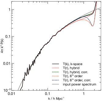
In Figure 6, we show the influence of the finite difference order on the initial power spectrum compared to traditional initial conditions using the k-space transfer function and a Fourier based Poisson solver. All initial conditions are for a particle discretisation of a box. The power spectrum was computed using the FFT on a cell density grid obtained via cloud-in-cell (CIC) interpolation from the particle positions. No deconvolution with the grid assignment operator was performed so that the CIC assignment leads to attenuation close to the Nyquist frequency of the mesh (outside of the plot) used to compute power spectrum in all cases (Jing, 2005). The uncorrected spectra using the real-space transfer function kernel show lack of power for wave numbers above even when using the hybrid Poisson solver which is equivalent to a pure FFT Poisson solver in the case of a periodic grid. This lack of power on such large scales is undesirable as it will suppress the growth of well resolved haloes.
Performing the finite volume correction in the case of the 6th order finite difference Poisson solver recovers all power below but (naturally) retains the lack of power on even smaller scales. In the case of the hybrid Poisson solver, the power is recovered on all scales down to . We observe a slight excess of power on the smallest scales.
Note that the motivation to apply these corrections is to match the properties of -space sampled initial conditions as closely as possible. However, they should not be understood as mandatory and are treated as options in our code. Applying the corrections for the respective Poisson solvers, the initial power spectra can be made to agree with the traditional exact -space sampled initial conditions with differences only on the smallest scales. We investigate the influence of these differences on -body simulations in Section 4. For the remainder of the paper, the respective corrections are applied for each method without explicit reference.
3.5.5 Spectral leakage and aliasing in FFT-Poisson solvers and Fourier space transfer functions
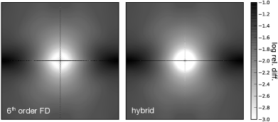
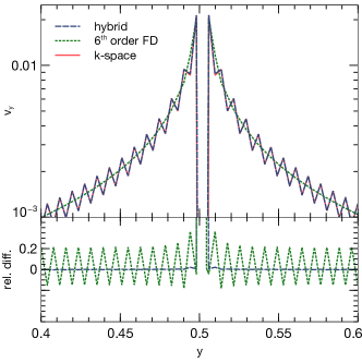
We investigate now the influence of using a real-space transfer function as well as a finite difference or hybrid Poisson solver compared to the standard method of using the -space transfer function and computing velocities. Velocities computed with equation (23) are not periodic in -space. Furthermore, the real space transform will be periodic and suffer from aliasing due to its Fourier space discretisation.
In order to assess the associated effects, we compute the velocity perturbation associated with a single peak at the center of a box at resolution. The peak represents a Dirac -function convolved with the transfer function. In Figure 7, we show the difference between the velocity field obtained with the real space transfer function using both 6th order multigrid and the hybrid Poisson solver, with respect to the velocity field obtained in the traditional way. We show two-dimensional slices in of the relative difference through the peak for the y-component of the velocity. Note that the velocity field is zero on the horizontal axis through the centre.
We first note that the relative difference falls below only in the central region. The 6th order multi-grid result has a slightly smaller central region with such low difference to the -space sampled results. Outside the central region, the relative difference rises to a maximum of per cent (outside the plane where the velocity vanishes), which is independent of the Poisson solver employed and thus a feature of the real-space transfer function. Indeed, it is the manifestation of the lack of spherical symmetry and aliasing (due to the finite number of samples) of the -space transfer function when transformed back to real space on a finite mesh.
We also observe spectral leakage showing up as a vertical feature passing through the centre. Spectral leakage is due to the non-periodicity in Fourier-space and thus the truncation of a non-periodic function at a finite wavenumber. The truncation leads to an oscillation at the Nyquist wavenumber in real space. In Figure 8, we show the central part of the velocity fields along the vertical axis of Figure 7 revealing the oscillatory nature. Spectral leakage is present whenever a -space exact Poisson solver is employed. Hence, the feature is not present in the multi-grid solution, which is periodic in Fourier space. Naturally, a similar feature is also present in the -space transfer function itself, when transformed to real space on a three dimensional mesh (see also Bertschinger, 2001).
Note that leakage in the velocity perturbations associated with a peak is likely to cause secondary correlations in the velocity field around rare high peaks but is unavoidable if no window function is used with the FFT Poisson solvers to truncate the spectrum smoothly at the Nyquist frequency. The use of such a window function (as e.g. the Hanning filter employed in Grafic-2, Bertschinger 2001) however reduces power at high frequencies which might be undesirable since it suppresses the small wavelength perturbations and thus the growth of haloes associated with them. We note that the finite difference approach has similar filtering properties with a relatively sharp cut-off in -space. Furthermore the finite difference operators are periodic in Fourier space. We do not consider the use of other window functions but perform our analysis of initial conditions generated with finite difference multi-grid and the hybrid Poisson solver in parallel throughout the remainder of this paper.
4 Error analysis
In this section, we first investigate the differences between the new methods described in Section 2 and 3 and the traditional approach of operating exclusively in Fourier space on various observables of cosmological -body simulations evolved over cosmic time as well as of a single galaxy cluster in order to ensure their proper performance in unigrid simulations. We then investigate the errors arising in nested “zoom-in” initial conditions generated with our method in both the initial conditions and in a re-simulation of a galaxy cluster.
4.1 Statistical properties of the cosmological simulations
In order to assess differences between initial conditions generated with the various methods, we ran Gadget-2 N-body simulation of a and a box with particles from redshift to . First order initial conditions (1LPT) were generated using the same random seeds. The power spectrum from which the initial conditions were generated in all cases has density parameters and , a Hubble constant , a normalization as well as a spectral index of and was computed using the fitting formula of Eisenstein & Hu (1998). We use Plummer equivalent softening lengths of for the runs and for the runs, respectively. These box sizes were chosen in order to probe both the highly non-linear regime, with the box, and the mildly non-linear regime with the box.
4.1.1 Evolution of the power spectrum
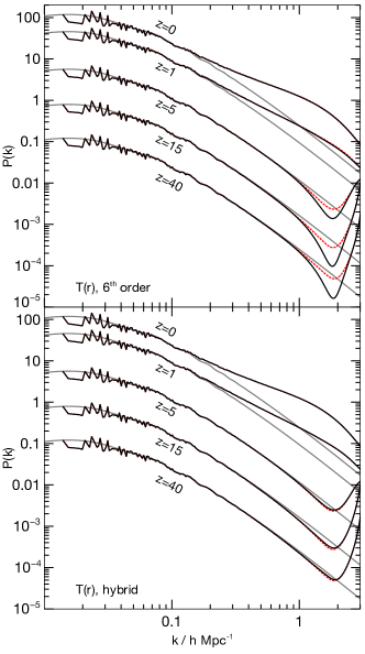
In Figure 9, we show the redshift evolution of the density power spectra for the box. We compare the linear theory evolution with the evolving power spectrum from initial conditions generated with the traditional -space sampling method, as well as generated with a real space transfer function convolution and both a 6th order finite difference and the hybrid Poisson solver.
As previously discussed in Section 3.5.4, the finite difference initial conditions show a significant suppression of power on the smallest scales. We see however that the power is immediately restored once the relevant scales enter non-linear growth and power is transferred from larger to smaller scales. The difference with respect to the -space initial conditions decreases over time and is no longer visible at . No wavenumbers below of the initial particle grid are affected at any time. Initial conditions generated with the hybrid scheme agree (almost) perfectly with the -space version. Again, the small initial difference also disappears completely once the relevant scales become non-linear.
Regarding large scales, we see no difference between the three methods, so that we focus our attention on a closer inspection of small scale behaviour in what follows.
4.1.2 The halo abundance
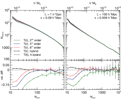
We compare halo abundance at a given mass between the various initial conditions. Haloes are identified using the Friends-of-Friends (FoF) algorithm (Press & Davis, 1982), grouping particles which are separated by less than times the mean inter-particle distance. Figure 10 shows the number of haloes in the simulations as a function of both halo particle number and halo mass. For both boxes and as expected, we see the strongest difference between the -space sampled initial conditions and those with 2nd order accuracy of the finite difference operators. In fact, halo abundance is lower up to 1000 halo particles. The histograms agree above and above halo particles for 4th and 6th order, respectively, with that of the -space method. The hybrid initial conditions agree over all mass ranges within per cent. Since halo abundance deviates from the Schechter function form also for the k-space initial conditions for haloes below 100 particles, it remains a question of future investigation whether the overabundance of the smallest mass haloes is a spurious result of the -space initial conditions.
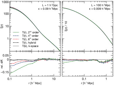
4.1.3 The small-scale correlation function
In Figure 11, we show the two-point correlation functions at . The two-point correlation function is defined as the excess probability (with respect to random) to find two particles in volume elements and separated by a co-moving distance ,
| (30) |
where indicates the mean particle number density. We computed the two-point correlation function using tree based sparse sampling thus computing more close-pairs than distant pairs for a subset of 1 per cent of the particles. Thus, statistical errors increase on larger scales.
For the box, our results indicate that is reduced by per cent at when using a 2nd order finite difference scheme, while for 6th order the reduction is only around per cent. Both 4th and 6th order results deviate by less than per cent at scales . For the highly non-linear regime probed by the runs, we do not find any significant differences. Gravitational interaction has wiped out any initial difference. We conclude that differences are negligible in the highly non-linear regime and as soon as mildly non-linear scales are well resolved.
4.2 Analysis of a galaxy cluster halo
In order to assess the influence of the real-space approach on the radial density profile of haloes, we investigate in more detail the properties of one cluster halo forming from initial conditions generated in the various ways in the box with particles.
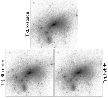
In Figure 12, images of the cluster at are shown for the three methods. Contrast in the images has been set in such a way as to make substructure most visible, white areas are not actually devoid of particles. Visually, the only difference between the three panels lies in the position of smaller substructure within the halo. All larger sub-haloes agree in their position. The overall shape of the halo is identical.
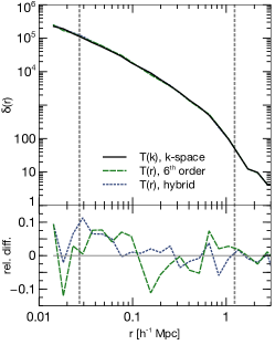
In order to asses differences more quantitatively, we show in Figure 13 the radial density profile centered on the densest particle (determined by averaging over 32 neighbours and weighted by a spline kernel) in each case. We find no systematic difference between either of the approaches. Differences are around 5 per cent and show no obvious bias. They are likely attributable to slight differences in the position of the substructure in the halo. These results further support the conclusion made in the previous section that differences between the real and the k-space approach are completely negligible in the highly non-linear regime.
The gross properties of the cluster halo are analyzed using the Amiga halo finder (AHF) (Knollmann & Knebe, 2009). In Table 3, we give the virial mass and radius , maximum circular velocity , the radius at which the circular velocity profile is maximal, the dimensionless spin parameter (Bullock et al., 2001), the three-dimensional velocity dispersion as well as the minor-to-major axis ratio , determined using the eigenvalues of the moment of inertia tensor (see e.g. Hahn et al., 2007). With the exception of , differences are around 1 per cent for all quantities investigated. It appears that is very sensitive to small changes in the density profiles leading to a difference of a few per cent in the finite difference case.
| , -space | , finite. diff. | , hybrid | |
|---|---|---|---|
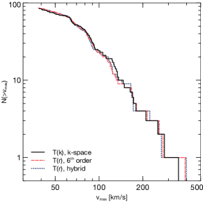
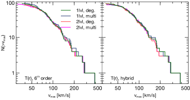
Finally, using AHF, we investigate the sub-halo population of the cluster. Since the finite difference approach suppresses slightly the formation of the smallest haloes (cf. 4.1.2), it is plausible that sub-haloes are affected as well, possibly even stronger. In Figure 14, we show the cumulative distribution of maximum circular velocity for all sub-haloes with at least 30 particles contained within the virial radius of the main cluster halo. We observe that the most massive substructure has a slightly lower for the -space initial conditions than for the others. The following sub-haloes, at next lower are identical. For the lower mass sub-haloes, the cumulative distributions agree, the simulation starting from the multi-grid initial conditions having slightly larger scatter than the one starting from hybrid initial conditions. In particular, we see no systematic deficiency of lowest mass haloes in the multi-grid case as might have been expected.
We conclude that differences in halo properties between the real-space and -space conditions are at the per cent level for gross properties and at the few per cent level for profiles and sub-halo mass functions. We do not observe any systematic bias.

4.3 Errors in nested initial conditions: Initial redshift
In this section, we analyze the errors in nested initial conditions computed with our method compared to a full-resolution solution with no local refinement. In order to compare our results with Bertschinger (2001), we decided to implement an identical set-up, where we replace white noise in cells outside the refinement region in the full-resolution set-up with the respective average value it has on the coarse grid in the “zoom-in” set-up. This ensures that identical white noise information is used in all cases, i.e. all the information that is in principle representable in the refined hierarchy. Note that naturally errors must arise at coarse-fine boundaries since the velocity and displacement fields must transition smoothly from fine to coarse resolution.
4.3.1 One refinement level
First, initial conditions are generated on a uniform grid for a box with white noise degraded to include identical information as in the “zoom-in” set-up to obtain the full-resolution answer. Next, another set of initial conditions is generated for a region of 0.2 times the box length at an effective resolution of while the remaining volume is treated at a resolution of . The high-resolution region comprises grid cells. In Figure 15, we show the error for the density field and the three components of the velocity for a slice in the plane through the centre of the refinement region. Colors correspond to the logarithm of the difference between the multi-scale solution and the full-grid solution in units of the standard deviation of the respective quantity on the full grid. In order to suppress the contribution from density convolution errors at the boundary, we padded the grids with additional grid cells at each boundary during the convolutions. This padding is however cut away before the potential is computed for the multi-scale hierarchy to ensure that the final velocity field is continuous and differentiable across coarse-fine boundaries. All results are shown for 1LPT initial conditions, the respective errors in the 2LPT case are qualitatively identical. We used the 6th order multi-grid for the results shown in this and the next section.
For the density, almost everywhere the difference is significantly below . We see that some errors at a few resulting from the interpolation of long-range components onto the finer grid. We find an RMS error of .
For the velocity components, again, errors are significantly below in the interior of the refinement region, apart from a few cells surrounding the boundary. Errors at the boundary are at most and arise due to the smooth coarse-fine transition in the refined set-up which is not present in the unigrid case. The RMS error is for all three velocity components. Since the interior errors are below , the RMS error over the entire refinement region is clearly dominated by only the errors at the boundary.
Errors for the hybrid Poisson solver are harder to compare since the long-range component from coarse grids is taken from the finite difference multi-grid solution so that it has no spectral leakage (see Section 3.5.5), while the same long-range component in the unigrid situation will show the spectral leakage in the form of oscillations at the Nyquist frequency around the smooth solution. This lack of spectral leakage in the long-range components completely dominates the error in the interior in a direct comparison of the unigrid and the multi-scale solution at a level of , no other errors are however introduced. Since leakage is an artifact of the finite mesh used for the FFTs, these differences are spurious and of no significance to our multi-scale approach to initial conditions.
In Figure 16, we show, for comparison, the error in the density and velocity component obtained with Grafic2 for the identical refinement set-up and identical random numbers as in Figure 15. We have used version 2.101 of the code and not removed or modified the standard antialiasing filter. Errors in density are about one, errors in velocity (and thus displacements) are about two orders of magnitude larger. Furthermore, unlike with our approach, errors are oscillatory and spread over the entire refinement domain. In addition, there is a significant vertical gradient at the level of several percent. We can only speculate about the sources of these errors. For the density field, our approach avoids the problem of aliasing and spectral leakage completely by operating purely in real-space. Furthermore, it produces by definition identical results for the component in the refined and the unigrid case. In addition, we have ensured that mass is conserved between grids thus avoiding long-range errors in the velocity components. Finally, the use of the adaptive multi-grid Poisson solver to compute velocities guarantees a solution of Poisson’s equation that is independent of the presence of a refined region if the mass field in the unigrid case is averaged with the restriction operator and then re-injected with the respective injection operator (averaging and straight injection in our case) in order to reflect the resolution in the refinement hierarchy.
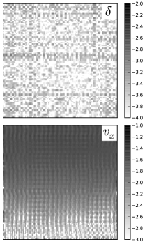
As mentioned before, Grafic2 also uses an antialiasing filter which severely suppresses power on small scales, so that the density and velocity fields generated are very smooth. We conclude that our new approach is an improvement by about two orders of magnitude in error reduction and the additional advantage that errors are completely confined to the boundaries.
In summary, with our method, errors in the interior are below with larger errors occurring at the boundary for the velocities due to the coarse-fine transition in the refinement hierarchy. It is particularly interesting to note that the velocity errors have no visible small scale components in the interior.

4.3.2 Two refinement levels
In this Section, we repeat the error analysis from above for a set-up of two nested refinement levels. The refinement region still has cells at an effective resolution of but is now embedded in an intermediate grid at effective resolution which is in turn embedded in the coarse grid with cells extending over the entire volume. The intermediate grid has an extent of cells beyond the edges of the finest grid. As before, we pad each refinement level with additional 8 boundary cells during the convolution step in order to avoid coarse-fine transition errors during the convolution. These boundary cells are again cut off before the potential is computed.
In Figure 17, we show the differences in the high-resolution region between the full-grid solution and the nested multi-scale solution. Density and velocity errors in the high-resolution region are roughly identical to the one level case above and below in the interior. We find RMS errors of for the overdensity field and for the three velocity components.
To summarize, we see no significant impact on the velocity field due to the introduction of additional refinement levels. All errors are completely localized at the coarse-fine boundaries. Regarding memory consumption, using double precision variables (8 bytes), we observed a peak memory usage of GBytes in unigrid mode (a double precision array requires 1 GByte of memory), MBytes in the case of the single refinement level set-up from above and MBytes in the two-level case from above, demonstrating the low memory footprint of our “zoom-in” approach to generate initial conditions.
4.4 Errors in nested initial conditions: Re-simulation of a galaxy cluster halo
In order to assess the influence of multi-scale initial conditions on the formation of a re-simulated object, we generate multi-scale initial conditions for one of the most massive clusters with mass in the box discussed before. We deliberately set the rectangular refinement region to include only the Lagrangian patch of the cluster halo. This will maximize the influence of both the coarse sampling of the large-scale tidal field and boundary effects on the formation of the cluster halo and allow us to estimate these effects. The refinement volume is a rectangular region of and was determined by following the FoF particles constituting the halo at back to the initial conditions and determining their bounding box rounded up/down to integer . Note that a sphere at mean density containing the mass of the cluster would have a diameter of .
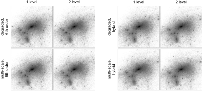
We perform Gadget-2 simulations with one level of refinement where the effective resolution in the high resolution region is and in the remainder of the box, as well as with two levels of refinement, where the high resolution region is surrounded by a layer of 16 particles thickness around each face at effective resolution that then drops to in the remainder of the box. In addition, we perform each simulation two times for both the multigrid finite-difference and the hybrid approach: once with the initial density field determined using the multi-scale convolution technique described in Section 3, and once with the density field determined at full resolution and then degraded (by averaging) to the same resolution as in the multi-scale setup followed by solving Poisson’s equation on the nested grid rather than the full grid. The latter produces completely negligible errors in the velocities and displacements inside the high resolution region. Differences from the full-grid initial velocities occur only in 2-3 cells at the boundary where the fields transition smoothly from fine to coarse resolution. All simulations are run with Gadget-2 and use a force softening length of for the high-resolution particles and for the other particles.
In Figure 18, we show the clusters at for all combinations of refinement set-up, Poisson solver and initial density generation method. We observe that the main halo as well as the most massive subhalos are consistent in position and size. The positions of some of the smaller halos are shifted and some smaller haloes seem to have merged in one set-up while they have not in some of the others. In general, visual differences are minimal. It is furthermore surprising that no systematic difference between the 1-level and the 2-level set-up can be seen. This is most likely a result of the padding region in the 2-level simulations at resolution which is identical to the 1-level simulations - the tidal influence of structures outside the padding region thus appears negligible and highlights the importance of adding padding.
Comparing Figure 18 with Figure 12, which shows the cluster in the unigrid simulations, we observe no obvious systematic differences apart from smaller sub-halo positions being slightly shifted. The overall shape of the cluster halo agrees very well between the re-simulations and the full box simulations.
We ran the Amiga halo finder (AHF) (Knollmann & Knebe, 2009) on the resimulated clusters and quote the same key values as in Section 4.2 to quantify the gross properties of the cluster halo in Table 4. As in the unigrid case, apart from , we find differences around 1 per cent or below for all quantities investigated.
| 6th order finite difference | |||||||
|---|---|---|---|---|---|---|---|
| 1 level, degraded | |||||||
| 1 level, multi-scale | |||||||
| 2 level, degraded | |||||||
| 2 level, multi-scale | |||||||
| hybrid Poisson solver | |||||||
| 1 level, degraded | |||||||
| 1 level, multi-scale | |||||||
| 2 level, degraded | |||||||
| 2 level, multi-scale | |||||||
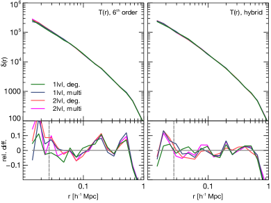
In Figure 19, we show the radial over-density profiles for the various cases. The lower panel show the relative difference with respect to the unigrid simulations. We observe no bias in either case. Scatter around the unigrid profile is larger for the finite difference case than for the hybrid initial conditions. For both methods, the scatter is slightly larger for the 2-level than for the 1-level set-up. Note that all “zoom-in” density profiles fall below the unigrid profiles in the last bin. This is due to the too small size of our refinement region as it is also present in the simulations generated by degrading the full density field. Despite the fact that it had been chosen too small, we find however not a single low resolution particle inside the virial radius, the first appearing at .
In Figure 20, we show the abundances of substructure as a function of maximum circular velocity within the virial radius of the cluster for all of the re-simulations. Differences between the 1 and 2-level results are at the level of several per cent for the finite difference case. The hybrid initial conditions show better agreement between the four runs. It is hard and beyond the scope of this paper to investigate to what degree these differences stem from simple changes of the sub-halo positions causing errors in determining their circular velocities (or masses) in the sub-halo finder.
We observe that the errors due to our multi-scale method, particularly with the hybrid Poisson solver, agree very well with the degraded initial conditions in both the one and two refinement level set-up. In particular, the scatter between the results from multi-scale density fields and degraded density fields is never larger than the difference between degraded initial conditions at one or two refinement levels itself. This leads us to conclude that the differences, apart from the introduction of an additional stochastic component, are dominated by the late-time evolution and not the initial conditions. In particular, we find no evidence that our method introduces systematic difference or bias in any of the investigated quantities.
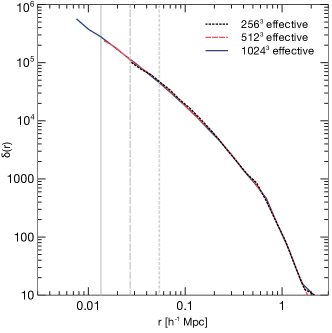
Finally, we investigate the convergence of the density profile at even higher resolution for the hybrid Poisson solver case. In Figure 21, we show the radial density profiles for a series of re-simulations that all have a base resolution of particles and one to three additional refinement levels. The profiles trace each other almost perfectly.
5 Baryon Initial Conditions
In this section, we discuss the generation of initial conditions for a two-component – dark matter and baryon – fluid. Linear perturbation theory predicts distinct amplitudes for baryon and CDM density fluctuations and also for their respective velocity fluctuations. We demonstrate that our approach using real-space transfer functions can be easily generalized for such a two-component fluid.
5.1 Density and velocity transfer functions
At high redshifts, at which initial conditions for cosmological simulations are typically generated, baryon density fluctuations are not yet exactly tracing the dark matter fluctuations (e.g. Yamamoto et al., 1998). Furthermore, baryon fluctuations are exponentially suppressed beyond the photon diffusion scale (Silk, 1968). These effects lead to a different shape of the baryon transfer function compared to the pure dark matter transfer function, particularly on small scales below .
Yoshida et al. (2003) demonstrated that the growth of density perturbations in the two-component fluid can only be correctly reproduced if besides the different initial amplitudes of density perturbations also the difference in initial velocities between the two components are respected. It is thus important that initial conditions for the two-component fluid reflect these important differences between baryons and dark matter and are thus able to reproduce the correct growth of fluctuations in both components consistent with the predictions from linear perturbation theories for those scales where perturbations are still small also with cosmological -body + hydrodynamics simulation codes. We defer a more detailed comparison with non-linear perturbation theory in two-component fluids (e.g. Somogyi & Smith, 2010) to later work.
For the two component fluid of baryons and dark matter, we determine both baryon and dark matter velocities using transfer functions, equivalent to the density perturbation transfer functions, that we construct in the following way. Using a Boltzmann solver, we solve the linearized equations of relativistic perturbation theory to obtain the velocity perturbations of the CDM and the baryon fluid. We adopt the notation of Ma & Bertschinger (1995) and kindly refer the reader to that publication for all details on the perturbation equations. We do not include the baryon temperature fluctuations as suggested by Naoz et al. (2010) as it is mainly relevant to perturbations with wavenumbers at and above the strongly Jeans damped regime. Using the results of linear perturbation theory, we define the two velocity transfer functions
| (31) | |||||
| (32) |
where is the conformal Newtonian potential for spatial metric perturbations and is the baryon velocity divergence. These transfer functions are constructed in such a way that at linear order the relation
| (33) |
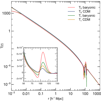
holds for the amplitude of velocity perturbations, i.e. they simply replace the density transfer functions in our algorithm when computing initial velocities as in Section 3.1.1. They furthermore allow the application of 2LPT (cf. Section 3.1.2), as they generate an “effective” source field for the velocity perturbations completely analogously to the relation between density and displacement. The respective real space transfer functions for all four fields are shown in Figure 22.
5.2 Evolution of Baryon perturbations
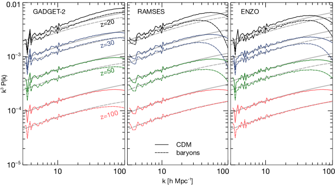
We now analyze the evolution of distinct baryon and CDM perturbations in two-component simulations using three commonly used cosmological simulation codes: Gadget-2 (Springel, 2005), Ramses (Teyssier, 2002) and Enzo (Bryan & Norman, 1997; Bryan et al., 2001; O’Shea et al., 2004). In each case, the initial conditions are generated at resolution for a box of comoving size with the same cosmological parameters as before and . The initial redshift is set to . For the grid codes (Enzo and Ramses), we do not allow for adaptive mesh refinement in order to avoid multi-scale density fields when computing the matter power spectra. In the SPH case (Gadet-2), we use a gravitational force softening of comoving for both baryons and CDM. Furthermore, SPH particles are placed on a staggered grid with respect to the CDM particles. In all cases, we assume a polytropic equation of state with adiabatic exponent , an initial temperature of , where is the mean molecular weight, and use neither cooling nor energy feedback. Note that Ramses, in our set-up, uses a piecewise linear method (PLM) for the hydrodynamics and mixed 2nd and 4th order gravity (2nd order in the Laplacian, 4th order in the gradients). Furthermore, we use the multidimensional monotonized central slope limiter (van Leer, 1977). Enzo uses a piecewise parabolic method (PPM) for the hydro and 2nd order gravity. We stop the simulations at and thus probe into the mildly non-linear regime.
The power spectra of the two-component perturbations are shown in Figure 23 at the initial and three subsequent redshifts, evolved with the respective codes. These power spectra have been computed on a grid using FFT with CIC interpolation for all particles, and directly from the baryon overdensity field for the grid codes. We do not correct for the loss of power due to the interpolation scheme and also do not smooth the SPH particles with their respective kernels. Thus, the baryon perturbations in the SPH case do not reflect the density perturbations seen by the SPH scheme, resolution thus appears to be significantly higher than for the grid codes, so that our results should not be used as an argument in favour or disfavour of either method.
We observe several differences between the codes. The SPH run with Gadget-2 shows excellent agreement with linear perturbation theory. The relative amplitude between CDM and baryon perturbations at any given mode matches very well even in the mildly non-linear regime at . It is not suprising that Gadget performs very well in our test since hydrodynamical forces are negligible in the regime probed and we thus only observe the performance of the tree-PM gravity solver.
In the case of Ramses and Enzo, CDM perturbations on the smallest scales grow slower than predicted by linear PT. This is however expected and a direct comparison with the Gadget results is unfair since we did not allow for refinement, and gravity forces are thus smoothed at the grid scale. For Enzo, the growth of CDM perturbations is more damped at small scales than in the Ramses run. This is most likely the result of the higher order of the gradient used by the Ramses Poisson solver.
For the baryon perturbations, small scales are growing slightly slower with Ramses than with Enzo. Again, this is to be expected since we use Enzo with PPM and Ramses with PLM. Also the type of Riemann solver and slope limiter used in Ramses has a slight effect, more diffusive limiters and solvers slightly decrease the power on the smallest scales. On large scales, all codes reproduce the correct growth of the perturbations, in very good agreement with linear PT.
To summarize, we observe that all three codes correctly evolve a baryon-CDM two-component fluid which starts with distinct density and velocity perturbations for each component. Differences that we observe with respect to the results from linear perturbation theory are attributable to the various numerical methods used in the simulation codes and not to the initial conditions.
5.3 Local Lagrangian approximation for the baryon density field
The density field sourcing the displacements and velocities in Lagrangian perturbation theory – which is a Gaussian random field – is inconsistent with the density field of the displaced particles – which is non-Gaussian. Using the Gaussian perturbation field as the initial baryon density field in grid based codes is thus inconsistent with the CDM perturbations. In this section, we describe an approach to prescribe initial gas density for the mesh cells based on the local Lagrangian approximation (LLA) that leads to consistency between the initial gas and dark matter density fields (see also Betancort-Rijo, 1991; Padmanabhan & Subramanian, 1993; Protogeros & Scherrer, 1997). Furthermore, it provides a natural way to prescribe the initial gas density on a grid also for 2LPT initial conditions.
The continuity equation is trivially fulfilled for a Lagrangian description of the fluid and simply reads We can however express the continuity equation in terms of the evolving fluid coordinates . It then becomes , where is the unperturbed mean density and is the density of the fluid element. Since the continuity equation is simply a volume integral, we can employ the change of variables theorem to express the left-hand-side also in terms of the initial position ,
| (34) |
Then, using eq. (10), the formal evolution of the density at the initial position of the fluid elements can be simply written as
| (35) |
where is the unity matrix. This implies that assumes a non-Gaussian distribution in general. In fact, will become singular whenever an eigenvalue of will become , corresponding to shell crossing along the respective axis. Since we use a first or second order Lagrangian perturbation theory approximation for the displacement field , eq. (35) is not exact and amounts to a “local Lagrangian approximation”. This means that, in general, mass will not be strictly conserved. We correct this by enforcing mass conservation by an a posteriori renormalization , where is the measured deviation from mean density. Typically, for sufficiently high initial redshift (as e.g. for the initial conditions used), the relative error is around 0.6 per cent and thus negligible (note that the error amounts to no more than per cent at much lower redshifts).
When computing for baryons, is sourced only by the baryon density perturbations, and so also contains only baryonic contributions. Note that application of the LLA does not change the baryon power spectrum.
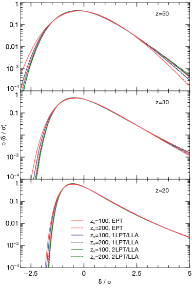
In Figure 24, we show the evolution of the probability distribution function (PDF) of the baryon overdensity field in an Enzo simulation using the same simulation parameters as above but for two different starting redshifts and . For both starting redshifts, we generate initial conditions in three different ways:
- EPT:
-
First order Lagrangian perturbation theory is used to initialize dark matter displacements and velocities as well as baryon velocities. The initial baryon density field is taken from Eulerian perturbation theory (which is common practice in grid based simulations). This baryon density field is initially Gaussian.
- 1LPT/LLA:
-
Again 1LPT is used, but now the initial baryon density field is computed according to equation (35), so that it is consistent with 1LPT. This initial baryon density field is no longer Gaussian.
- 2LPT/LLA:
We find that a similar transient behaviour as that between 1LPT and 2LPT for pure CDM simulations (cf. eg. Crocce et al., 2006; Tatekawa & Mizuno, 2007) can be observed. The skewness of the density field is underestimated when starting at with the initially Gaussian field (EPT). This is somewhat improved when starting at higher redshifts. When using an initial density field that is consistent with 1LPT, the skewness is boosted so that the dependence of the PDF on the initial redshift of the simulation becomes smaller. When using 2LPT and LLA, no significant dependence of the PDF on the starting redshift can be observed. Note that we show the results for the baryon density field directly taken from the simulations rather than a density field that was smoothed with an aperture filter. Filtering with a finite apperture however leads to almost identical results, the skewness is underestimated at high redshifts independent of scale.
In summary, Eulerian perturbation theory leads to an underestimation of the skewness of the baryon density PDF at high redshifts. When using the LLA for the baryons, a PDF is imposed that is consistent with Lagrangian perturbation theory. In particular, as has been shown already for dark matter simulations, the density PDF becomes much less sensitive to the initial starting redshift when using 2LPT. Using the local Lagrangian approximation, consistent initial baryon density fields can be construed.
6 Summary & Conclusions
We have presented and implemented a method to generate real-space sampled initial conditions for nested grids, extending prior work by Pen (1997), Bertschinger (2001) and Sirko (2005). These initial conditions are suitable for “zoom-in” cosmological simulations of structure formation with several levels of refinement that allow the study of single cosmological objects, such as e.g. groups and clusters of galaxies, single galaxies, or first stars, in a cosmological context at very high resolution while maintaining a small computer memory footprint.
Apart from the general advantage of real-space sampled initial conditions discussed by Pen (1997) and Sirko (2005), namely a correct reproduction of real-space statistical properties, such as the two-point correlation function and mass variance in spheres, we demonstrate that our multi-scale convolution approach for nested grids has very favourable error properties: (1) no interference of different modes between different refinement levels, and (2) errors confined to coarse-fine boundaries. We find RMS errors of velocity/displacement fields in the refined region at the order of in units of the standard deviation of the respective fields which is an improvement of about two orders of magnitude over previous approaches.
In order to determine particle displacement and velocity fields, at first and second order Lagrangian perturbation theory, we followed two approaches. First, a pure multi-grid Poisson solver is used. We show that the finite volume discretization it assumes leads to a suppression of perturbations at the smallest scales that can however be corrected by a deconvolution. Second, a hybrid Poisson solver is developed, which uses an adaptive multi-grid algorithm for inter-level gravity and an FFT-based Poisson solver for the finest grid. This hybrid approach leads to no suppression of small scale perturbations. Analyzing statistical properties of unigrid simulations for which initial conditions have been generated with the two different approaches, we find however that non-linear objects are not sensitive to the lack of power at these very small scales and differences are only seen in the mildly non-linear regime and at the lowest halo masses. We conclude that our real-space based approach is well suited also for initial conditions for unigrid simulations.
In order to verify the accuracy of nested initial conditions generated with our method, we investigated the properties of a galaxy cluster both in a unigrid simulation and a “zoom-in” simulation with one and two levels of refinement. We find that the gross properties of the cluster, such as virial mass, radius, spin, shape and velocity dispersion, are recovered at per cent level or better in the re-simulations. Density profiles show no bias with scatter at the level of a few per cent, mainly attributable to slight changes in the positions of sub-structures in the re-simulations. We also find that the sub-halo mass function is recovered with an accuracy of a few per cent in all re-simulations, and observe that the hybrid Poisson solver performs slightly better than the pure multi-grid approach. We thus conclude that our algorithm does not introduce bias or unreasonable scatter in observables that will be deduced from such a re-simulation and will thus provide a reliable tool to study the internal structure of cosmological observables at high resolution in large cosmological volumes.
Finally, we study the inclusion of a baryonic component in our approach by generalising the use of real space transfer functions also for distinct baryon and CDM density and velocity perturbations. We demonstrate that our approach reproduces the evolution expected from linear perturbation theory correctly. Furthermore, we propose to set the initial baryon density field based on a local Lagrangian approximation which is consistent with Lagrangian perturbation theory of first or second order and which greatly reduces the dependence of the baryon density field on the starting redshift of the simulation, thus reducing transient behaviour.
Acknowledgments
The authors thank Hao-Yi Wu for help with testing the code and invaluable feedback, Romain Teyssier, John Wise, Anatoly Klypin, Matthew Turk and Adrian Jenkins for comments and discussions that helped to improve both the paper and the code. Finally, the authors thank the referee, Simon Prunet, for very valuable suggestions to improve the presentation of the paper. All simulations were run on the Orange cluster at KIPAC/SLAC. This work was partially supported by NASA ATFP grant NNX08AH26G, NSF AST-0808398 and NSF AST-0807075. TA acknowledges financial support from the Baden-Württemberg-Stiftung under grant P-LS-SPII/18.
References
- Abel et al. (2002) Abel T., Bryan G. L., Norman M. L., 2002, Science, 295, 93
- Bernardeau et al. (2002) Bernardeau F., Colombi S., Gaztañaga E., Scoccimarro R., 2002, Phys. Rep., 367, 1
- Bertschinger (2001) Bertschinger E., 2001, ApJS, 137, 1
- Betancort-Rijo (1991) Betancort-Rijo J., 1991, MNRAS, 251, 399
- Bouchet et al. (1995) Bouchet F. R., Colombi S., Hivon E., Juszkiewicz R., 1995, A&A, 296, 575
- Bournaud et al. (2010) Bournaud F., Elmegreen B. G., Teyssier R., Block D. L., Puerari I., 2010, MNRAS, 409, 1088
- Brandt (1973) Brandt A., 1973, in Cabannes H., Teman R., eds, Proceedings of the Third International Conference on Numerical Methods in Fluid Mechanics Vol. 18 of Lecture Notes in Physics, Multi–level adaptive technique (MLAT) for fast numerical solution to boundary value problems. Springer–Verlag, Berlin, pp 82–89
- Brandt (1977) Brandt A., 1977, Math. Comp., 31, 333
- Bryan et al. (2001) Bryan G. L., Abel T., Norman M. L., 2001, arXiv:astro-ph/0112089
- Bryan & Norman (1997) Bryan G. L., Norman M. L., 1997, in D. A. Clarke & M. J. West ed., Computational Astrophysics; 12th Kingston Meeting on Theoretical Astrophysics Vol. 123 of Astronomical Society of the Pacific Conference Series, Simulating X-Ray Clusters with Adaptive Mesh Refinement. pp 363–+
- Buchert et al. (1994) Buchert T., Melott A. L., Weiss A. G., 1994, A&A, 288, 349
- Bullock et al. (2001) Bullock J. S., Dekel A., Kolatt T. S., Kravtsov A. V., Klypin A. A., Porciani C., Primack J. R., 2001, ApJ, 555, 240
- Ceverino & Klypin (2009) Ceverino D., Klypin A., 2009, ApJ, 695, 292
- Crain et al. (2009) Crain R. A., Theuns T., Dalla Vecchia C., Eke V. R., Frenk C. S., Jenkins A., Kay S. T., Peacock J. A., Pearce F. R., Schaye J., Springel V., Thomas P. A., White S. D. M., Wiersma R. P. C., 2009, MNRAS, 399, 1773
- Crocce et al. (2006) Crocce M., Pueblas S., Scoccimarro R., 2006, MNRAS, 373, 369
- Davis et al. (1985) Davis M., Efstathiou G., Frenk C. S., White S. D. M., 1985, ApJ, 292, 371
- Di Matteo et al. (2008) Di Matteo T., Colberg J., Springel V., Hernquist L., Sijacki D., 2008, ApJ, 676, 33
- Efstathiou et al. (1985) Efstathiou G., Davis M., White S. D. M., Frenk C. S., 1985, ApJS, 57, 241
- Eisenstein & Hu (1998) Eisenstein D. J., Hu W., 1998, ApJ, 496, 605
- Fedorenko (1961) Fedorenko R. P., 1961, Z. Vycisl. Mat. i. Mat. Fiz., 1, 922
- Hahn et al. (2007) Hahn O., Porciani C., Carollo C. M., Dekel A., 2007, MNRAS, 375, 489
- Hahn et al. (2010) Hahn O., Teyssier R., Carollo C. M., 2010, MNRAS, 405, 274
- Hamilton (2000) Hamilton A. J. S., 2000, MNRAS, 312, 257
- Hockney & Eastwood (1981) Hockney R. W., Eastwood J. W., 1981, Computer Simulation Using Particles. McGraw-Hill
- Hoffman & Ribak (1991) Hoffman Y., Ribak E., 1991, ApJ, 380, L5
- Jenkins (2010) Jenkins A., 2010, MNRAS, 403, 1859
- Jing (2005) Jing Y. P., 2005, ApJ, 620, 559
- Katz et al. (1994) Katz N., Quinn T., Bertschinger E., Gelb J. M., 1994, MNRAS, 270, L71+
- Knollmann & Knebe (2009) Knollmann S. R., Knebe A., 2009, ApJS, 182, 608
- Ma & Bertschinger (1995) Ma C., Bertschinger E., 1995, ApJ, 455, 7
- Martin & Cartwright (1996) Martin D. F., Cartwright K. L., 1996, in Electronics Research Laboratory Memorandum UCB/ERL M96/66 Solving poisson’s equation using adaptive mesh refinement. University of California, Berkeley
- Miniati & Colella (2007) Miniati F., Colella P., 2007, J. Comput. Phys., 227, 400
- Munshi et al. (1994) Munshi D., Sahni V., Starobinsky A. A., 1994, ApJ, 436, 517
- Naoz et al. (2010) Naoz S., Yoshida N., Barkana R., 2010, arXiv:1009.0945
- Navarro & White (1994) Navarro J. F., White S. D. M., 1994, MNRAS, 267, 401
- O’Shea et al. (2004) O’Shea B. W., Bryan G., Bordner J., Norman M. L., Abel T., Harkness R., Kritsuk A., 2004, arXiv:astro-ph/0403044
- Padmanabhan & Subramanian (1993) Padmanabhan T., Subramanian K., 1993, ApJ, 410, 482
- Peebles (1982) Peebles P. J. E., 1982, ApJ, 263, L1
- Pen (1997) Pen U., 1997, ApJ, 490, L127+
- Pichon et al. (2010) Pichon C., Thiébaut E., Prunet S., Benabed K., Colombi S., Sousbie T., Teyssier R., 2010, MNRAS, 401, 705
- Press & Davis (1982) Press W. H., Davis M., 1982, ApJ, 259, 449
- Protogeros & Scherrer (1997) Protogeros Z. A. M., Scherrer R. J., 1997, MNRAS, 284, 425
- Prunet et al. (2008) Prunet S., Pichon C., Aubert D., Pogosyan D., Teyssier R., Gottloeber S., 2008, ApJS, 178, 179
- Salmon (1996) Salmon J., 1996, ApJ, 460, 59
- Scoccimarro (1998) Scoccimarro R., 1998, MNRAS, 299, 1097
- Seljak & Zaldarriaga (1996) Seljak U., Zaldarriaga M., 1996, ApJ, 469, 437
- Silk (1968) Silk J., 1968, ApJ, 151, 459
- Sirko (2005) Sirko E., 2005, ApJ, 634, 728
- Somogyi & Smith (2010) Somogyi G., Smith, R. E., 2010, Phys. Rev. D, 81, 023524
- Springel (2005) Springel V., 2005, MNRAS, 364, 1105
- Springel et al. (2005) Springel V., White S. D. M., Jenkins A., Frenk C. S., Yoshida N., Gao L., Navarro J., Thacker R., Croton D., Helly J., Peacock J. A., Cole S., Thomas P., Couchman H., Evrard A., Colberg J., Pearce F., 2005, Nature, 435, 629
- Stadel et al. (2009) Stadel J., Potter D., Moore B., Diemand J., Madau P., Zemp M., Kuhlen M., Quilis V., 2009, MNRAS, 398, L21
- Talman (1978) Talman J. D., 1978, Journal of Computational Physics, 29, 35
- Tatekawa & Mizuno (2007) Tatekawa T., Mizuno S., 2007, JCAP, 12, 14
- Teyssier (2002) Teyssier R., 2002, A&A, 385, 337
- Trottenberg et al. (2001) Trottenberg U., Oosterlee C. W., Schuller A., 2001, Multigrid. Academic Press
- Turk et al. (2009) Turk M. J., Abel T., O’Shea B., 2009, Science, 325, 601
- van Leer (1977) van Leer B., 1977, Journal of Computational Physics, 23, 263
- Wise & Abel (2008) Wise J. H., Abel T., 2008, ApJ, 685, 40
- Yamamoto et al. (1998) Yamamoto K., Sugiyama N., Sato H., 1998, ApJ, 501, 442
- Yoshida et al. (2008) Yoshida N., Omukai K., Hernquist L., 2008, Science, 321, 669
- Yoshida et al. (2003) Yoshida N., Sugiyama N., Hernquist L., 2003, MNRAS, 344, 481
- Zel’Dovich (1970) Zel’Dovich Y. B., 1970, A&A, 5, 84