Ultraviolet filtering of lattice configurations and applications to Monte Carlo dynamics
Abstract
We present a detailed study of a filtering method based upon Dirac quasi-zero-modes in the adjoint representation. The procedure induces no distortions on configurations which are solutions of the euclidean classical equations of motion. On the other hand, it is very effective in reducing the short-wavelength stochastic noise present in Monte-Carlo generated configurations. After testing the performance of the method in various situations, we apply it successfully to study the effect of Monte-Carlo dynamics on topological structures like instantons.
1 Introduction
In Quantum Field Theory the path integral is supported on distributions. Nevertheless, the semiclassical method aims at obtaining a reduced path integral space, labelled by smooth configurations. This is not in contradiction since the weights account for all the stochastic fluctuations around them. In the weak coupling limit this methodology works successfully for many theories. In the case of QCD, one might consider, for example, a dilute gas of instantons parametrised by its positions and sizes [1]. Classically, the distribution is Poissonian with a uniform distribution in space, a scale invariant distribution in sizes and a classical weight for each new instanton which is the exponential of minus its action. This is not the appropriate path integral measure though, since the integration over gaussian fluctuations around an instanton forces to replace the action by the free energy. This induces a size dependence dictated by the renormalization group. Nevertheless, such a reduced path-integral space, although successful in predicting a non-zero topological susceptibility, crucial for the solution of the U(1) problem, does not reproduce other phenomena believed to be present in the full theory, such as Confinement. Presumably a picture based upon the classical vacuum () with isolated lumps is a poor description of the true vacuum. Indeed, the quantum weights determined by perturbation theory already tell us that instantons prefer to grow and overlap with others [2, 3]. A possible modified scenario, in which instantons are close to each other but preserve their individuality is the instanton liquid model [4]-[7]. In any case, a non-dilute picture is much harder to handle and introduces considerable complications into the semiclassical roadmap. The difficulty is not necessarily an impossibility. For example, the space of self-dual configurations contains structures with all sort of overlapping and non-diluteness, but still can be parametrised in terms of a few parameters known as ADHM data [8]. The dilute instanton pattern is included as a corner in this much richer configuration space. Other self-dual configurations look very different. In particular, some can be described by an ensemble of lumps of fractional topological charge 1/N. These other configurations not only lead to a non-vanishing topological susceptibility, but also to a non-zero value of the string tension. These and other attractive properties motivated a proposal for the structure of the QCD vacuum by our group based on fractional topological charge structures [9]. The proposal is not devoid of problems since a realistic description of the vacuum should allow the simultaneous presence of topological objects of both signs, which are not classical solutions.
Lattice Gauge theory provides a first-principles framework to study non-perturbative aspects of the theory. It has been very successful in supporting QCD as the basic theory underlying strong interactions. Furthermore, it has enabled precision tests of the predictions of the Standard Model, a necessary ingredient for detecting evidence for any extension [10]. However, there are still many aspects which remain to be understood, some of which play a major role for candidate technicolor theories, for example. A priori, the lattice approach can also help in solving the questions referring to the validity of the semiclassical approach and the elucidation of whatever classical structures can account for the properties of the vacuum. Unfortunately, the general statements made at the beginning of this section imply that Monte Carlo generated lattice configurations contain a high level of stochastic short-wavelength noise. This noise completely masks the long-wavelength topological structure information. This justifies the necessity for finding a procedure that would enable one to reduce this noise and surface the underlying long-wavelength structures present in them.
A filtering method is a procedure which takes as input a gauge field configuration with stochastic noise and produces a new one which preserves its long-range and topological structure and substantially reduces the short-range stochastic noise. Many are the methods that have been explored to achieve this purpose. They range from those which iteratively smooth the gauge field, like smearing [11]-[15], cooling [16]-[22], or the Wilson flow [23], to those that attempt at reproducing the topological density through a truncation of the spectral density of operators like the Dirac [24]-[31], or the Laplacian operators [32]. Ideally, any such method should produce a clean picture of the underlying long-range structures without introducing biases and distortions of the final data. However, all of the methods mentioned above have been criticized in this respect since the amount of filtering they introduce depends on ad-hoc parameters such as the number of cooling or smearing steps, or the cut-off at which the filtering operators are truncated. Still, they have been used quite successfully in analyzing global as well as local properties of the QCD topological structures. Recent reviews of the results obtained employing these methods as well as comparison of the performance of different filtering procedures can be found i.e. in Refs. [33]-[35]. The aim of the present work is to explore and develop a particular implementation of a filtering method, introduced in Ref. [36], which does not suffer from the ambiguities mentioned above. The basic point which motivated the proposal is the idea that an optimal filtering method should leave smooth classical configurations invariant. Note that this is a non-trivial requirement, not satisfied for instance by any finite truncation of the spectral density of the Dirac operator in the fundamental representation. The key point exploited in Ref. [36] is that Supersymmetry equates the density of certain zero-modes of the Dirac operator in the adjoint representation with the gauge field action density [37]. However, in the presence of noise both observables behave in a very different fashion. On general grounds it is to be expected that the density of the supersymmetric zero-modes tends to suppress the effect of high frequency noise as compared to the action density itself, thus providing a filtered image of the latter. In Ref. [36] the idea was presented and a series of tests were carried on to show that the method works satisfactorily.
In this paper we take this idea and develop one of its most elegant and well defined implementations. This can be translated to the lattice by making use of the overlap Dirac operator [38], which shares many nice features with its continuum counterpart. Preliminary results have been presented in [39]-[41]. The structure of the paper is as follows. In the following section we explain the definition of the filtering procedure in its continuum version and discuss why it is supposed to produce a filtered image of the gauge action density even in the presence of noise. Section 2.1 provides the details of the lattice implementation of the procedure in terms of the overlap Dirac operator. In section 3 we carry on a systematic study of how the filtering affects smooth configurations, both solutions of the classical equations of motion and others that are not, such as instanton - anti-instanton pairs. A basic goal is to quantify the distortions and biases that the method could introduce. The final test, presented in section 4, corresponds to the analysis of noisy configurations that have been obtained by applying several heat-bath Monte Carlo sweeps to a smooth instanton configuration. We will show that the method spectacularly succeeds in filtering away the ultraviolet noise.
Having tested the method, we embark in section 5 in a possible application which is novel and might have important implications in hot problems such as the observed slow thermalization of Monte Carlo updates at high values of the coupling [42]-[44]. Starting with a classical configuration we apply a series of heat-bath steps at several values of the coupling. This introduces stochastic noise which, even for very small number of heat-bath steps, masks the classical configuration from which we started. The updating procedure also induces a motion along the space of classical configurations, changing its moduli parameters. In particular, for instantons, which have been our main focus, the position and size of the instanton performs a stochastic motion. Our method can be used to study this motion and test if it follows the theoretical expectations. Results are quite impressive and might allow the numerical determination of the relative quantum weights of other families of classical configurations.
The results and conclusions of the paper are summarised in the last section.
2 Construction of the filtering method
As explained in the introduction, the main idea underlying the method is the relation between gauge field structure and zero-mode density implied by Supersymmetry. More precisely, we make use of the fact that given a solution of the classical equations of motion, the Dirac operator in the adjoint representation has a zero-mode, called the supersymmetric zero-mode, whose density coincides with the action density [37]. As a matter of fact, decomposing the mode into its two chiral components, the corresponding densities follow the shape of the self-dual and anti-self-dual parts of the action density. The general details are given in Ref. [36] and will be explained below. For the sake of clarity we will start by describing the method for the particular implementation which we are using in this paper.
Given a gauge field configuration , we can construct the corresponding Weyl operators and for the adjoint representation. The Weyl operator is given by , with and the Pauli matrices. The other operator , is minus the adjoint of . The Weyl matrices and , satisfy the relations
| (2.1) |
where and are the ‘t Hooft symbols (summation over repeated indices implied).
Using the Weyl operators we can construct the following hermitian positive operator:
| (2.2) |
The spectrum of this operator is doubly degenerate. This follows from the reality of the covariant derivative in the adjoint representation. Given an eigenvector , one can construct an orthogonal one of the same eigenvalue as . The two bi-spinors can be combined into a single quaternionic eigenvector . We are identifying the space of quaternions with a real subspace of the space of complex matrices. The Weyl matrices are a basis of the quaternionic space. Using this basis the operator can be seen as a matrix whose components can be obtained by making use of Eq. (2.1). Having presented the basic terminology, we proceed with the explanation of the method.
The basic object, in terms of which the filtering procedure is formulated, is , where denotes the projector onto the 3 dimensional subspace generated by the Pauli matrices. In components it is given by:
| (2.3) |
The right hand side can be processed using the expression for the commutator of covariant derivatives:
| (2.4) |
This restriction preserves the real, hermitian, positive semi-definite character of the operator.
The filtered image of the self-dual part of the action density is defined as the density of the eigenmode of lowest eigenvalue of the operator :
| (2.5) |
Indeed the components in colour space are real numbers, and the density is given by
| (2.6) |
The whole construction can be repeated for the other chirality. The main difference is that the and symbols are exchanged. Hence the final formula becomes
| (2.7) |
The corresponding mode is the filtered image of the anti-self-dual part of the gauge field. For the ease of notation we will be referring to the lowest eigenvectors of the operators as the adjoint filtering modes or AFM modes.
Having presented the method, we will explain the reasons why it is supposed to produce a filtered image of the gauge field configuration. To start with, we will focus on smooth configurations which are solutions of the classical equations of motion. In this case the filtered image should produce an undistorted image of the configuration itself. This is precisely the role played by Supersymmetry and the supersymmetric zero-mode. Given a solution of the euclidean classical equations of motion, we can decompose its field strength into its selfdual and anti-selfdual parts, as follows:
Combining the equations of motion with the Bianchi identities one sees that the self-dual part satisfies the equation:
| (2.8) |
and a similar equation, with replaced by , for the anti-selfdual part. Introducing a quaternionic field , one can show (using the properties of the ‘t Hooft symbols) that the previous equation can be written as
| (2.9) |
This equation expresses that is a zero-mode of the Dirac equation in the adjoint representation. This is the supersymmetric zero-mode, whose density is exactly proportional to that of the self-dual part of the field. Obviously, is also a zero-mode of the positive hermitian operator. Noticing that is a linear combination of the Pauli matrices alone, one concludes that is also a zero-mode of the operator . Now, one understands better the role played by the projection onto the three-dimensional subspace leading to the construction of . Indeed, the Weyl operator might have many zero-modes. This is necessarily the case for classical solutions having positive definite topological charge (number of adjoint zero-modes ). However, the supersymmetric zero-mode is indeed unique in that its quaternionic field is traceless, at all points of space and for all colour components. In other words it is a purely imaginary quaternionic field. This property, called reality condition in Ref. [36], lies at the heart of our method. We lack a general proof of uniqueness, but in the particular case of self-dual gauge fields, the ADHM construction allows us to give formal expressions for all the zero-modes. In quaternionic notation they can be written as . The reality condition amounts to demanding . This, except for some limiting cases, indeed singles out the supersymmetric zero-mode. Our approach in this paper has been to directly impose the reality condition by looking at the projected operators . Alternatively, one could start by exploring the low-lying spectra of the operator, imposing a posteriori the reality condition to select the supersymmetric zero-mode. This is the practical approach implemented in Ref. [36]. Although the results obtained were quite satisfactory, it requires dealing with the multiplicity of the zero-modes and turns out to be less efficient and numerically more costly than the present proposal.
What do we know about the excited states of the spectrum of the operator. In general, for a finite volume, we expect a gap to develop in the spectrum. The gap goes to zero for large volumes, but the corresponding limiting states become non-normalizable. The operator has a single point discrete spectrum and a gapless continuum spectrum. Furthermore, the eigenmodes would look rather structureless and easily distinguishable from the supersymmetric zero-mode. We will see how these expectations are realized in our numerical results.
Certainly a possible analytical testing ground is that of a single SU(2) instanton. Here the only scale is clearly , so that we might use it as a unit of lengths and energies. The operator can be rewritten using the formula of the covariant Laplacian for an instanton in SU(2) [2]
| (2.10) |
In the previous formula:
and , where summation over repeated indices is understood. In addition and are the generators of SU(2) in the adjoint representation acting respectively on the colour or on the spinorial indices.
If we restrict to purely radial eigenvectors and split upon eigenstates of the direct product representation , with isospins , we get:
| (2.11) |
We might write the rotationally invariant eigenvectors as:
| (2.12) |
The eigenvalue equation then reduces to
| (2.13) |
Obviously for , is a solution of vanishing eigenvalue. This is the expected supersymmetric zero-mode. It is easy to see that there are in addition 5 non-normalizable zero-modes for and .
Up to now, we have just analysed the behaviour of the filtering procedure for solutions of the classical equations of motion, for which the filtering mode is just the supersymmetric zero-mode. For other smooth configurations the lowest eigenvalue will not be zero. Indeed, if we take the self-dual part of the gauge field and apply the operator to it, we get
| (2.14) |
which only vanishes if the current, , vanishes. From here we get an upper bound on the minimal eigenvalue of :
| (2.15) |
If the smooth configuration is made of local structures which are approximate solutions of the classical equations of motion, the current would be very small in those regions and the filtered mode will be close to the self-dual action density. The limit to this situation would be the region in which level crossing appears. We will explore this situation in our numerical analysis, to be presented later.
In order to understand the behaviour of the operators for non-classical configurations, one could study small perturbations about the classical solutions: . To derive the appropriate formula it is better to regard as the projected version of . The eigenvalue equation, to leading order in , takes the form
| (2.16) |
Projecting onto one realizes that vanishes (hence it is order ). The equation for the eigenvector is
| (2.17) |
The right-hand side can be evaluated to
| (2.18) |
Now, without loss of generality we might impose the background gauge condition on . With this we can rewrite the right-hand side as
| (2.19) |
After several operations one arrives at the equation
| (2.20) |
where .
To see the filtering properties of the method, we might consider a deformation involving high frequencies. For that purpose we make proportional to for high values of . The corresponding field strengths , will then be proportional to . Thus, in the corresponding action density the noise terms are amplified with a factor . Let us now look at the expected behaviour of the filtered mode . The right-hand side of Eq. (2.20) will also contain terms proportional to . To solve the equation we should decompose this term into eigenstates of the operator. The decomposition should be dominated by states of high eigenvalue, which are essentially given by plane waves . Since, the field-strength of the zero-mode is smooth, the typical wavelengths involved are . The same reasoning tells us that the corresponding eigenvalue of the operator is . Applying, these considerations to Eq. (2.20) we conclude that goes like . The new filtered mode density has a suppression of the added noise. This is precisely the desired effect, which makes our method a filtering procedure for the gauge field configurations.
2.1 Lattice implementation
There are two important ingredients involved in the construction of the operators: chirality and the reality of the covariant derivative. In implementing the method on the lattice it is convenient to preserve these properties. This can be achieved by using the overlap operator [38] as lattice Dirac operator. This will be explained below. Some results obtained with this procedure were presented in Ref. [40].
The lattice version of the operator is given by
| (2.21) |
where and is the projection onto the space of purely imaginary quaternions as before. The overlap Dirac operator is given by the formula:
| (2.22) |
where is a hermitian, unitary matrix given by:
| (2.23) |
and . The matrix is the standard massless Wilson-Dirac operator in the adjoint representation given by:
| (2.24) |
where and label points in the 4-dimensional lattice of spacing , and is the unit vector in the direction. The gauge field links in the adjoint representation can be obtained in terms of links in the fundamental as follows:
| (2.25) |
where are the generators of SU(N) in the fundamental representation with the standard normalization . Notice that the links in the adjoint representation are real orthogonal matrices.
The overlap Dirac operator is known to satisfy -hermiticity and the Ginsparg-Wilson relation
| (2.26) |
These two conditions imply that commutes with . The positive and negative chirality components are the lattice counterpart of and .
Finally, we should verify that the projection onto the purely imaginary quaternions operates in the same way as in the continuum. The reality of the gauge field links in the adjoint representation implies the double-degeneracy of the eigenvalues of . This follows from the equation
| (2.27) |
where is the charge conjugation matrix satisfying . Eq. (2.27) also holds for the overlap Dirac operator and for . In the Weyl representation of the Dirac matrices
| (2.28) |
the matrix can be chosen as . Thus, following the same procedure as in the continuum, the chiral components of can be seen as a matrix acting on quaternions. Restriction to the subspace of purely imaginary quaternions leads to the matrices defined in Eq. (2.21).
In our lattice implementation of the overlap operator, we have used the rational expansion for the matrix proposed in [45, 46]:
| (2.29) |
where and . The action of the matrices over a vector is computed by using the method of multiple shifts described in [47]. As a compromise between performance and stability we have taken and the tolerance parameter that controls the conjugate gradient accuracy is taken to . In order to minimize the storage needs, we use the two-pass algorithm proposed by Neuberger [48]. The pseudo-code necessary for the implementation is well described in Ref. [48].
In order to compute the low-lying spectrum of the operators we have used the conjugate gradient algorithm [49]. The eigenvectors are computed with an accuracy such that:
| (2.30) |
with . This guarantees no appreciable errors in the eigenvector densities. The speed at which convergence is achieved depends very much on the gauge field configuration and on the initial vector for the conjugate gradient algorithm. Typically, for the cases analysed in the paper, the computer time needed to determine the lowest eigenvector grows as , with a proportionality constant that increases as decreases. In some cases we have seen that a suitable choice of the initial vector for the conjugate gradient can reduce this time by a factor of 5.
To check that our results are not biased by the choice of the matrix expansion, we have repeated the computation of the low-lying spectrum on some of the configurations with the Lanczos algorithm proposed in [50]. The results obtained by both methods are compatible within errors.
Finally, we comment on the choice of the Wilson-Dirac mass term . Most of our results were obtained for . This value is a compromise which allows the filtering method to detect fairly small instantons without sacrificing performance [39, 41]. Nevertheless, we have done several tests to check the dependence of our results upon the value of . In all cases, including noisy and smooth gauge field configurations, no significant changes are observed on the density of the AFM. This contrasts with the results in Ref. [31] obtained using the modes of the Dirac operator in the fundamental representation as filtering modes. In that case, the claim is that the value of monitors the amount of filtering obtained for the configuration.
3 Testing the method with smooth configurations
In this section we will test the numerical implementation of the filtering method on a set of smooth lattice configurations. We will focus on two generic situations. First, we will look at lattice configurations that correspond, in the continuum limit, to solutions of the classical equations of motion. This includes discretized instantons and calorons [51, 52] as well as higher topological charge objects. The filtering method should work well in this case, but the analysis will allow to quantify discretization and finite volume effects. Second, we will analyze smooth configurations which are not solutions of the continuum equations of motion. We will focus in particular on the case of instanton - anti-instanton pairs, testing the ability of the filtering method to detect structures in both chiral sectors. In all cases we will analyze the low lying spectrum of the operators, paying particular attention to the occurrence of level-crossing that could disturb the identification of the adjoint filtering mode.
3.1 Classical configurations
The filtering operator is designed to select the supersymmetric zero-mode if applied to classical backgrounds. This is guaranteed in the continuum but, for the method to work, it is essential that this property is preserved when both the operators and the classical configurations are discretized. Lattice artefacts can be considered as a particular case of the deformations discussed in section 2. We expect them to induce an lifting of the AFM eigenvalue and a small modification of its density through mixing with the excited states. Although this contamination goes away in the continuum limit, it is important to quantify the distortions it may introduce in the procedure.
In what follows we will analyze several and , SU(2) configurations discretized on the lattice. We will show that the method spectacularly succeeds in identifying classical lumps down to sizes of the order of two lattice spacings. Results will be presented for SU(2) instantons but we have also checked that the filtering procedure works well for other classical solutions as finite temperature calorons [51, 52], or fractional charge instantons [53, 54].
3.1.1 Single instanton configurations
For the purpose of the test we have generated a set of , SU(2) lattice instanton configurations for several lattice volumes () and two different sets of boundary conditions. In addition to a periodic torus (p.b.c.) we have also considered a torus with twisted boundary conditions (t.b.c.) [55], corresponding to and . The reasons to employ twisted boundary conditions are twofold. To start with, the gap in the spectrum of the filtering operator is strongly dependent on the boundary conditions. It is easy to understand why this is the case by analysing the spectrum on a trivial background. For t.b.c. the set of classical vacua is discrete and the spectrum has a gap of size , for and finite box size . Periodic boxes, on the contrary, have a continuum of classical vacua [56, 57] which support a continuum of constant density adjoint zero-modes. On the background of instanton configurations, these vacuum zero-modes become quasi-zero-modes for and can give rise to unwanted level-crossing in the spectrum. This situation is avoided in the twisted case, where the gap in the spectrum pushes any level-crossing to very large values of . There is a second reason to select twisted instead of periodic boundary conditions for the analysis of instantons. On a finite periodic box there is a restriction over the allowed topological charge of classical solutions, and is not feasible [58]. Although this restriction disappears in the thermodynamic limit, it gives rise to finite size effects that can shift considerably away from zero the lowest eigenvalue of the filtering operator. This limitation disappears, however, as soon as one imposes a non-zero twist.
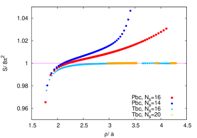


The results we will present correspond to instanton configurations of various sizes generated by cooling, an iterative update process that monotonically decreases the lattice action [16]. Since the lattice breaks the scale invariance, the fate of instantons under cooling depends crucially on the choice of lattice action employed in the cooling algorithm [20]. One can take advantage of this and use cooling to modify at will the instanton size parameter . In this paper we have made use of the -cooling method proposed in Ref. [20]. It employs a variant of the Wilson action containing and plaquettes with relative coefficients tuned to control the scale violations of the lattice action. In particular, is the choice that eliminates these corrections. Figure 1 displays the dependence of the integrated instanton action versus the instanton size for several lattice volumes. For t.b.c. the deviation from the continuum instanton action amounts to less than one part per mille for instantons of size larger than . In that range we expect very small distortions in the spectrum of the operator. The situation is not as good for periodic boundary conditions since, as we have just discussed, there are no exact classical solutions with on a finite periodic box. For this reason the deviation from the continuum action is generically much larger than with t.b.c.. The results that will be presented in this section correspond to several representative twisted and periodic configurations selected among the ones displayed in these plots.
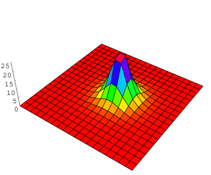
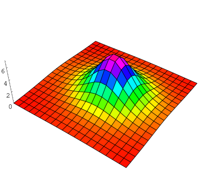
For all the configurations analyzed we have computed the four lowest eigenvalues in each chiral sector. The sector of negative chirality is structureless. For positive chirality, as expected, one of the eigenvalues is distinctively smaller than the others. Its eigenvector provides the adjoint filtering mode (AFM) which should correspond to the supersymmetric zero-mode whose density reproduces the instanton action density. A comparison between the density of the AFM and the self-dual part of the action density is displayed in figure 2 for two instantons of sizes and , with and twisted boundary conditions. The qualitative agreement is impressive. For a more quantitative comparison we give in table 1 the values of the instanton parameters obtained from the densities of the AFM (, ) and the self-dual part of the gauge field strength (, ). They have been extracted by fitting the 1-dimensional instanton profiles to the data, following the procedure described in the appendix. Differences in the extracted instanton locations are negligible. As for the sizes, the differences remain much smaller than those associated to different fitting procedures - see figure 15 in the appendix.
-0.0007 0.0004 -0.0005 0.0008 2.992 2.977 -0.0001 0.0001 0. 0.0001 6.175 6.190
We proceed next to present a detailed analysis of the effect of the numerical implementation on the spectrum. It is important for the success of the method that no level-crossing takes place between the lowest eigenvalue and the excited states since this would induce a misidentification of the supersymmetric zero-mode. We will discuss first the case of twisted boundary conditions which from this point of view provides a much cleaner situation. As discussed before, the spectrum of the operator is gapless in the infinite volume limit with a continuum spectrum that corresponds to non-normalizable states. For finite volume however there is a finite gap of order and no level-crossing is expected. We will analyze in what follows how lattice artifacts modify this expectation, and we will see that in the worst case situation level-crossing will only occur for very large lattice sizes . Figure 3 displays, for twisted boundary conditions and two different lattice sizes, and 20, the lowest (left) and first excited (right) eigenvalues of the operator. Let us first focus on the analysis of the lattice artifacts on the AFM eigenvalue (). In the plot it is displayed as a function of the instanton size in lattice units: . The line drawn in the plot corresponds to a fit of the form:
| (3.1) |
with coefficients , and . It describes well the data for and shows that the eigenvalue of the filtering mode approaches zero in the continuum limit, as expected. Results are given for instantons of size larger than to avoid problems in the convergence of the conjugate gradient algorithm.
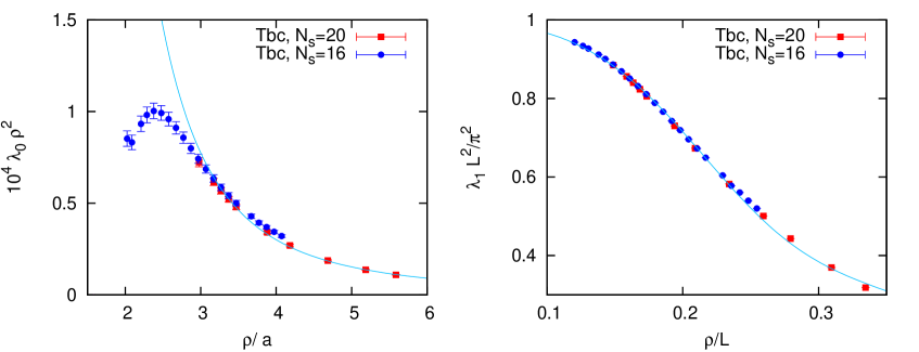
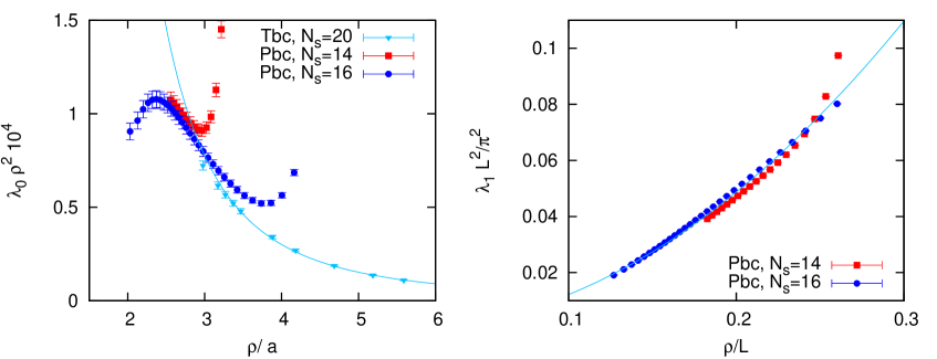
With respect to the first excited eigenvalue a comparison between the and the results shows that it scales as . The data can be fitted to
| (3.2) |
where , and . From the fits to the two eigenvalues we can extract the ratio and estimate when it will become of order 1. We find that for instantons of size () the level-crossing will take place for extremely large values of the lattice volume, ().
The situation is much worse for periodic boundary conditions since in that case the gap in the spectrum goes to zero with decreasing . The results are presented in figure 4, where we display the two lowest eigenvalues of the filtering operator. The AFM eigenvalue, displayed on the left plot, matches the twisted result, Eq. (3.1), for small . It becomes however strongly affected by finite size effects for , as a consequence of the absence of exact solutions in the periodic case. The first excited eigenvalue, displayed on the right plot, goes to zero as . The fit in the figure corresponds to:
| (3.3) |
with . Combining this fit with the one describing the lattice artifacts Eq. (3.1), we can again estimate when the ratio between the two eigenvalues becomes of order 1. In this case it happens for rather small values of : for () the level-crossing will take place at ().
3.1.2 Two instanton configurations
In this subsection we will study other classical solutions. As in the previous case, the filtering method is bound to work in the continuum, so that our goal is mostly that of exploring possible problems associated to the discretization. This is a necessary step previous to any application to Monte Carlo generated configurations. Our study has focused in one situation which might potentially cause problems. This occurs whenever the gauge field configuration contains widely separated structures. It is to be expected that in this case the gap narrows down, since every isolated structure should give rise to a quasi-zero-mode of the operator. There is still a unique zero-mode associated to the supersymmetric zero-mode, but lattice corrections might induce unwanted mixing, whose effects we want to explore.
For definiteness we have concentrated our study in the case of two instantons (I-I) at variable separations. For the analysis we have prepared a set of SU(2) instanton configurations, by applying the following engineering techniques. Typically, we start with a couple of instantons on a lattice of size . The configurations are glued along the time direction, and subsequently cooled until the total action drops to a value close to , signalling that the configuration is approximately a solution of the classical equations of motion. The gluing can be done at variable separation among the two instantons, and this is not substantially altered by the cooling process. Finally, we end up with a collection of configurations on a lattice and with periodic boundary conditions. Notice that, in contrast to the case, in this case there are indeed classical solutions in the continuum living in a box without twist.

We studied the low-lying eigenstates of the operator for the afore-mentioned set of configurations. Our results for the spectrum, displayed in figure 5, agree nicely with our expectations. There is a unique zero-mode (up to lattice corrections) for all I-I separations. The first excited eigenvalue, however, depends strongly upon separation , dropping to zero as this separation gets large. This dependence can be fitted to , where is the average size of the two instantons. The second excited eigenvalue, on the contrary, does not depend significantly upon the separation and is presumably mostly determined by box-size and boundary conditions.
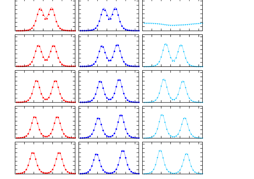
Our interpretation of the results is substantiated by the structure of the two lowest eigenvector densities, displayed in figure 6 for several values of the separation . The 1-d profiles represent the integral of the densities over the spatial directions. For comparison, the spatial integral of the self-dual part of the action density is also displayed. Two regimes are clearly observed. For an I-I distance of , the situation is similar to the one instanton case: The ground state density matches the self-dual action density, and the first excited state corresponds to a nearly constant mode. For larger separations a level crossing takes place in the excited spectrum and both densities display the distinctive two instanton profile of the action density.
Let us examine these results in the light of our expectations. In the limit of infinite separation each instanton () has an associated supersymmetric quasi-zero-mode , given by its corresponding electric field. As the instantons approach each other, the ground state of , which is an exact zero-mode, is given by the symmetric combination . The antisymmetric combination should correspond to the first excited state. Both densities coincide with the self-dual action density (except for minor corrections in the region where the instantons overlap). On close observation, however, we notice that the density profiles on figure 6 show slightly different weights for each of the two peaks in both the ground state and the excited state. This is presumably an effect of the discretization. Lattice artefacts induce a mixing of both states, which can be estimated by diagonalizing the operator in the subspace spanned by and . Writing the perturbed states as:
one obtains
where is the gap between the unperturbed states. The lattice artefacts enter through the expectation value: . We can estimate the size of by replacing in the denominator of this expression the actual gap, extracted from the data in figure 5, and for the numerator the typical size of the lowest eigenvalue on a instanton background. For our I-I configurations we estimate that the maximal mixing is attained for the largest separation , being of order . A direct determination based on the relative heights of both peaks gives a value of , in remarkable agreement with our crude estimate.
Although the possible alteration of the peak heights, for the case of sufficiently isolated structures and corresponding small gaps, is a matter of concern, we want to emphasize that it is not an insurmountable difficulty, once the origin of the problem is pinned down. Indeed, our determination of instanton parameters is largely insensitive to this normalization. This is clearly shown in table 2, where we collect the size parameters of both instantons extracted from fitting the action density and the two lowest eigenmode densities. As described in the appendix, the fitting has been done using the shape around the peaks of the 1-d profiles obtained by integrating the densities in the spatial directions. The continuous lines in figure 6 correspond to a superposition of the 1d-instanton profiles given by Eq. (A.3) in the appendix, with parameters, including normalization, determined from the fits.
3.8624 - 3.9201 3.8045 - 3.8600 1.58 - 3.8450 3.7621 3.8946 3.8048 3.7090 3.9700 2.03 0.013 3.6222 3.6272 3.6982 3.6362 3.6511 3.7139 2.72 0.020 3.6641 3.6531 3.7315 3.6717 3.6630 3.7498 3.22 0.036 3.6732 3.6522 3.7313 3.6570 3.6391 3.7344 3.75 0.040
To summarize, the filtering procedure succeeds in reproducing the action density. We have studied a distortion in relative normalization of the profiles induced by lattice artifacts, which is present when the instanton separation is large enough. There might be several ways to cope with it, once we know its presence and origin. In particular, possible improvements of the operator, which reduce the size of lattice artefacts, will also reduce this effect.
3.2 Smooth non-classical configurations
Having tested successfully the performance of the filtering method on classical configurations, we now turn to the analysis of smooth backgrounds that are not solutions of the classical equations of motion. The prototype example is an instanton-anti-instanton (I-A) pair which approaches a classical solution only in the limit of infinite I-A separation. Although in this case we do not expect exact zero-modes of the operators, we will show that one eigenvalue in each chiral sector remains in general significantly smaller than the others. This is so even for configurations in which the instanton and the anti-instanton overlap considerably and allows to unambiguously select the adjoint filtering modes. As we will see, the densities of the AFMs correctly reproduce the self-dual and anti-selfdual parts of the action density.

For the analysis, we have generated several SU(2) I-A configurations with different I-A separation on a lattice with periodic boundary conditions. The set has been obtained by letting a well separated I-A pair annihilate under cooling. The initial configuration is engineered by gluing along the time direction an instanton with the anti-instanton obtained from it by time reflection. In the process of destruction of the pair the action monotonically decreases from values close to to less than , a point after which one can no longer identify the I-A lumps in the gauge action density.
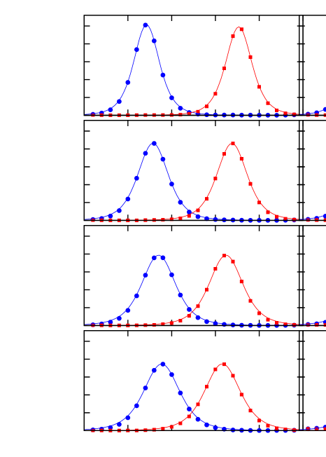
Let us present first the analysis of the spectra. Figure 7 displays the two lowest eigenvalues of the operator as a function of the inverse I-A overlap: . A similar picture is obtained in the negative chirality sector. The lowest eigenvalue increases with I-A overlap but a clear gap is maintained as far as . This allows to clearly identify the AFM. We will discuss the closing of the gap later on but let us concentrate now on the AFM densities. They are represented in figure 8 for several characteristic stages in the process of I-A annihilation corresponding to , 2.42, 1.87, and 1.59. We present on the left the 1-dimensional profiles of the self-dual and anti-selfdual parts of the action density compared with the AFM densities displayed on the right. The agreement is in all cases very good, even for the lowest plot that corresponds to the maximal I-A overlap in figure 7, above which level crossing takes place. We extract the (anti) instanton parameters by fitting these 1-d profiles following the procedure described in the appendix. The results are presented in table 3, and the corresponding fits represented by the continuum lines on the plot. Even for the extreme case with largest overlap, the difference between the size parameters extracted for the AFM modes and the gauge densities amounts only to 10, decreasing down to less than 1 for .
1.965 3.2116 3.1240 3.1941 3.1045 3.35 1.906 3.8008 3.7744 3.7489 3.7223 2.42 1.787 4.3250 4.3028 4.1402 4.1105 1.87 1.659 4.8835 4.7766 4.3804 4.3500 1.59
One final remark is that, unfortunately, the level-crossing is controlled not only by the growth of the lowest eigenvalue with the I-A overlap, but also by the finite volume dependence of the first excited eigenvalue . We can estimate in general when it takes place. The lowest eigenvalue can be fitted to
| (3.4) |
where the fit corresponds to the continuum line in figure 7. The first excited eigenvalue is expected to behave as for twisted, and as for periodic boundary conditions (see respectively Eqs. (3.2) and (3.3)). By requiring we obtain:
| (3.5) | |||||
| (3.6) |
For example, the identification of a pair with requires for periodic boundary conditions, and for the twisted case. Once again the use of twisted boundary conditions pushes away the region in which level crossing takes place.
4 Testing the method with noisy configurations
We now come to the crucial test on the filtering method. Our ultimate goal is to apply the method to Monte-Carlo ensembles and extract from it a clear picture of its underlying long-range topological content. The only way in which one could trust the results is if one has previously tested the method in a controlled situation. It is not just a question of recovering the long-range information stored in the configuration, but also of making sure that the filtering procedure does not introduce important distortions in the main parameters describing the underlying topological structure.
Our proposed strategy is the following. Starting from a smooth configuration, we begin to apply Monte Carlo updating steps to it. We limit ourselves to large values of and a small number of Monte-Carlo heat-bath sweeps to guarantee that the initial configuration is not destroyed in the process, and that only statistical noise is added to it. In this and the following section we will test the ability of our filtering method to eliminate the stochastic noise present in heated configurations, and make use of the information provided to monitor the thermalization process itself.

In practise, we have concentrated most of our work in pure SU(2) gauge theories. Our initial configurations are in all cases instantons of various sizes obtained with periodic or twisted boundary conditions. If the size parameter of the instanton is small compared to the size of the four-dimensional box no significant change of the instanton shape is expected with respect to the infinite volume continuum instanton.
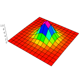
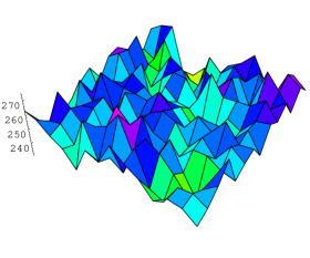
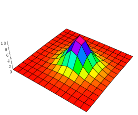
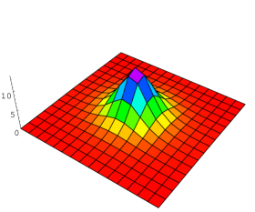
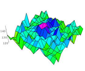
We have applied heat-bath sweep updates to these smooth configurations. Short wavelength stochastic noise comes in very fast and short range observables (as the average plaquette value) quickly approach values close to those corresponding to thermalized ensembles. The size of the noise is of order , but even for relatively large values of it dominates the value of the action density, and the trace of the initial instanton appears to be washed out. This can be clearly observed in figure 9. The left pictures display the self-dual part of the action density of a smooth instanton integrated in two directions. The center figures display the same quantity after applying heat-bath sweeps to it, at two different values of ( with for the top figure, and with for the bottom one). Notice the tremendous change in scale which follows from the size of stochastic noise, even at these relatively large values of . Nevertheless, the original instanton is still there. The right figures display the image obtained after applying our filtering method to the configurations depicted in the center figures. Remarkably, the shape looks rather similar to the one of the original instanton, and certainly not noisier.
Although the results look spectacular we are not satisfied by just obtaining a clean smooth picture of the underlying instanton. We aim at having full control of the possible distortions introduced in the parameters (position and size) of the initial instanton. This will be analysed in the next section, where we will describe the ability of the filtering method to extract the stochastic motion performed by these moduli parameters under heating.
On the basis of the perturbative analysis of section 2 we knew that the filtering method should act appropriately for configurations which are deformations of solutions of the classical equations of motion. However, why should the method still work so well in these cases in which the size of the noise is rather large? In the remaining of this section we will provide a partial answer to this point.
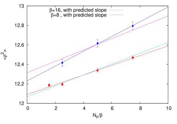
For that purpose, we studied the effect of heating on the low-lying spectrum of the operator . The initial smooth configuration was taken to be an SU(2) instanton of size on a lattice of length , employing both periodic and twisted boundary conditions for the reasons explained previously. Starting from these smooth configurations we performed heat-bath sweeps with the Wilson action at various values of , ranging from to . For each initial configuration and value of we repeated the procedure 10 times with independent random seeds, and averaged the values obtained for the four lowest eigenvalues of over them. The results are displayed in figure 10. The continuous line gives the result of a fit to the two smallest eigenvalues up to for each boundary condition. For twisted boundary conditions we get:
| (4.1) | |||||
| (4.2) |
and for periodic boundary conditions we obtain:
| (4.3) | |||||
| (4.4) |
Notice that as goes to infinity the results approach those obtained for smooth instantons in the previous sections. There is a zero-mode (up to lattice cut-off effects) for both boundary conditions, and a gap which is volume dependent and strongly dependent on boundary conditions. For large values of , the lowest eigenvalue is proportional to as predicted by perturbation theory. The leading correction to the higher eigenvalues seems to behave in the same way. Perturbation theory allows that deformations lead to a modification of the excited eigenvalues proportional to . Nevertheless, since the noise introduced by the heat-bath method is stochastic and has both signs, we find it quite possible that in this case the correction to the eigenvalue is also of order as our data seem to indicate. Furthermore, it is remarkable that a fit to the dependence, depicted as a continuum line in figure 10, shows that the coefficient of the term is very much compatible for the first and second eigenvalue and both boundary conditions. The same applies for the coefficient of the term. There is no particular reason why there should be no term as well, but adding it to the fit gives a coefficient which is compatible with zero, and a larger value for the per degree of freedom.
Some final comments are in order. The lowest eigenvalue of the operator depends mildly on the value of . Typically, it starts to rise for the initial heat-bath steps, but quickly saturates to a fixed value. The value also depends slightly on the choice of the heat-bath action. Taking the improved action instead of the Wilson action only affects the coefficients by 10%.
The most remarkable feature shown by figure 10, is that the gap remains approximately constant for all values of . This is the reason why our method works well in all that range. Had level crossing occurred, our filtered mode would have lost the trace of the underlying instanton, and failed dramatically. In the following section we will go one step further and investigate how the heat-bath process and the filtering affect the instanton parameters.
5 Analysing Monte Carlo dynamics
In this section we will present the results of a detailed study of the effect of heat-bath updates and subsequent filtering upon the collective parameters describing an instanton: its position and size parameter . The philosophy is similar to that presented in the previous section but taking spatial care in minimising systematic errors and increasing the statistical significance of the results.
Our initial smooth instanton configuration was generated by -cooling [20] with in order to reduce lattice artifacts. Different instantons sizes have been studied, but most of our data has been obtained for . This is a safe intermediate value, far from the , in which the instanton soon evaporates and the lattice action is strongly dependent of the value, and the larger values where finite volume starts affecting the shape and stability. The lattice size was taken as and we used twisted boundary conditions (, ) for the reasons explained before.
The Monte Carlo updating procedure consisted on a heat-bath algorithm based on the classically improved lattice action described previously. Two values of , and , were used in our analysis. These relatively large values of ensure that the heat-bath updating mostly adds stochastic noise to the configuration, but does not destroy it or create new structures. Having two values of allows to quantify how much of these fluctuations are gaussian, allowing us to extrapolate the results for lower values of . Finally, we have studied the evolution of the sample for different number of heating steps , by applying the filtering procedure to all the noisy configurations at specific values of and extracting from the AFM density the value of the instanton parameters, using the methodology described in the appendix.
How should the distribution of instanton parameters look like for the heated sample? It is quite clear that, in addition to generating gaussian fluctuations, the heat-bath dynamics should also generate modifications of the moduli parameters characteristic of the underlying smooth configuration. In particular, for instantons, both the location and size parameter should behave stochastically as a result of the updating procedure. Up to lattice artifacts the position should describe a random walk with no drift term. On the other hand, the quantum fluctuations should not be flat in space, because it is precisely the quantum fluctuations introduced by the updating procedure what leads to the size dependence of the free energy computed by ‘t Hooft [2]. Although, the updating procedure is discrete, we expect that for sufficiently large values of and of the number of updating steps the evolution could be well modelled by a Langevin equation. The equation for the displacement parameter being purely a Wiener process, with a probability distribution satisfying the heat equation. More precisely, if we started with a gaussian distribution, it will remain gaussian at all times, with constant mean value and a dispersion behaving as
| (5.1) |
The slope parameter measures the velocity of the diffusion process and is a characteristic of the updating procedure. On general grounds we know, however, that it is proportional to the square of the size of the noise. Thus, for our particular case it should go like .
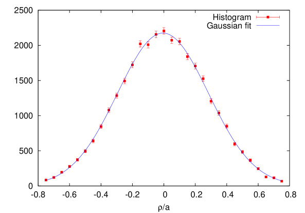
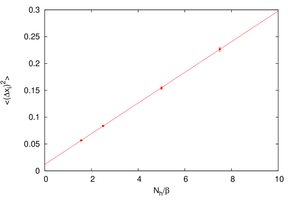
Let us see how our data behaves with respect to these expectations. For that purpose, starting from our smooth instanton of size , we generated 7885 independent trajectories by applying a sequence of up to 120 heat-bath steps with . We stored the configurations after 25, 40, 80 and 120 heat-bath sweeps. To the four sets of 7885 configurations we applied our filtering procedure. In all cases the filtered image showed a clear peak close to the position of the initial instanton similar to that displayed in figure 9. For each filtered image we extracted the position and size of the corresponding instanton following the procedure specified in the appendix. Finally, we performed an statistical analysis of the results. In particular, we computed the displacement of the center of the instanton obtained from the AFM relative to the position of the initial instanton. The data agrees nicely with the expectations of a gaussian distribution. For example, figure 11 shows the statistical distribution for of the displacement putting the 4 components of the displacement in the same plot to increase the statistics. The data are compared with a gaussian distribution fitted to the data. The per degree of freedom is 1.15. For the remaining values of similar results were obtained with -pdof of order 1. Finally, the mean value and dispersion of the distribution were obtained either directly or by a fit to a gaussian distribution, with compatible results. The mean value obtained was always smaller than 0.01 lattice spacings with no particular dependence. On the contrary, the dispersion was observed to grow linearly with the number of heat-bath steps. Figure 12 shows the values of the dispersion as a function of . The solid line is the result of a fit to a straight line having per degree of freedom smaller than 1. The fit is given by:
| (5.2) |
with , and . The relation of with the slope parameter entering Eq. (5.1) is given by . All results are given in units of the lattice spacing.
To test the dependence we repeated the procedure for , , and heat-bath sweeps, and 3940 trajectories. The results are qualitatively the same as described for . The dispersion is fitted to . Notice that the slope is compatible with the one obtained at , in agreement with the hypothesis of gaussian fluctuations. One feature that differs from our Langevin model is the fact that the intercept is non-zero. It is not surprising that the continuous Langevin description does not apply during the first few steps. Indeed, the agreement is expected only in the limit with fixed. This seems to affect mostly the intercept. Apparently the intercept behaves as . In any case, this small change is the only one which could reasonably be attributed to the distortions associated to the filtering method itself.
Now we proceed to the analysis of the evolution. In this case we expect a drift due to the -dependence of the free energy. According to the calculation of Ref. [2] the probability distribution of the size parameter should behave as
The first factor comes from the scale invariant distribution in collective coordinates, while the second one follows from the exponential of the action with a renormalized coupling constant computed at the scale . Indeed, the value 22/3 follows from the leading-order beta function. The free energy is then given by minus the logarithm of this term. Thus, the Fokker-Planck equation which describes the stochastic evolution of the distribution in is given by
| (5.3) |
In this case, even if one starts with a gaussian distribution in at time equal zero, it will cease to be gaussian at longer times. Nevertheless, numerical integration of this equation reveals very small deviations from gaussianity during the range of times corresponding to our heat-bath updates. The drift term shows up in the prediction that the mean value becomes an increasing function of time. This function is approximately a straight line in the appropriate time range. The dispersion, , shows also a (very approximate) linear growth with time, with a slope given by . One can circumvent even these minor deviations by computing . According to the Fokker-Planck equation one can easily deduce that this quantity should grow exactly linearly with time:
| (5.4) |
The corresponding slope should be higher than by a factor that gives a measure of the beta function:
| (5.5) |
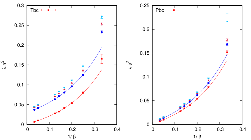
Let us now see how the data behaves with respect to our expectations. In figure 13 we plot the value of for our and data, together with a linear fit to the data. The slopes are compatible (0.0168(4) for and 0.0175(16) for ). Again the intercept scales as .
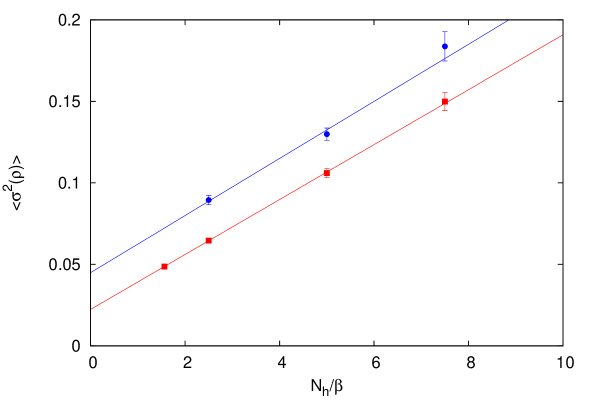
The most crucial aspect is the behaviour of which, according to our expectations, should grow linearly with a slope which is 10/3 larger than the one of . In figure 14 a fit to the data is performed showing, for , a slope of . This gives a ratio of instead of . This is less than 2 sigma away from the expected value, and gives in any case a value incompatible with the one observed for the dispersion . We can safely claim that we have obtained numerical evidence for the predicted dependence of the free energy with . The data at show the same trend, although this time the slope overshoots and the ratio is rather . All the parameters of the linear fit to our data are collected in table 4. The errors quoted include both statistical (using jack-knife) and systematic effects coming from correlation upon fit-parameters.
We have done other checks at different values of but with smaller statistics. It is impossible in this case to determine the drift in the mean value of , but given that the dispersions are affected by much smaller errors, we can extract meaningful values of and from the data. In particular we generated 500 trajectories at , and . In all cases we obtain good linear fits for the dispersion in displacement and in size . The parameters of the fits are collected in table 4 and are reasonably compatible with each other. Although, the range in is small and the errors are large, we can safely conclude that the slopes are not strongly dependent on the value of .
Our data predicts the dependence of the displacement and as a function of the number of heating steps. The results can be extrapolated to lower values of . Although, as decreases we expect non-linear dependencies in it would be very surprising that the results change by orders of magnitude. What are the possible implications of these results? Suppose one has a Monte Carlo generated configuration with a particular instanton content. Applying heat-bath sweeps to this configuration the positions and sizes of instantons will change approximately according to the pattern derived in this paper. Eventually either by displacement or by growth the instantons will meet anti-instantons and with a finite probability annihilate. The last steps could be very fast, but for large initial separations most of the time will be employed in the stochastic motion depicted in this paper. Other processes are possible. Equal sign instantons might merge into new structures and even percolate as a result of the growth in . In addition, dislocations can be created which might eventually develop into new instantons and change the value of the topological charge of the configuration. Finally, one can have the reverse phenomenon, since small instantons have a finite probability of decreasing in size and disappearing through the holes of the lattice. It is clear that only once these processes have acted sufficiently can we approach a thermal distribution of the topological structure. The autocorrelation time for this type of processes are much larger than those affecting local quantities such as the mean value of the plaquette. Assuming that does not depend on , as our data seems to support, we can conclude that, in order to reach changes in displacements and sizes which are given by appropriate values in physical units, we need to perform a number heating steps given by:
| (5.6) |
This grows very fast for large values of due to the presence of the factor in the denominator. This is a typical critical slowing down phenomenon. The factor of adds to the difficulty, since it is of order 30-60 for displacements and sizes respectively. If we input the characteristic values of and one can provide an estimate of the corresponding autocorrelation times.
Confs 16 3.5 7885 25, 40, 80, 120 0.192(7) 0.0286(4) 0.357(15) 0.0168(4) 8 3.5 3940 20, 40, 60 0.17(2) 0.032(2) 0.36(5) 0.0175(16) 16 3.25 500 5, 10, 20, 50, 100 0.10(1) 0.031(1) 0.20(4) 0.019(2) 16 3.78 500 5, 10, 20, 40 0.14(2) 0.034(2) 0.28(6) 0.023(4) 16 2.8 500 10, 20, 30, 40 0.06(1) 0.0314(5) 0.17(2) 0.0189(15)
6 Conclusions and Outlook
In this paper we have studied a filtering method proposed in Ref. [36]. We have considered a simple and precise definition of the filtered profiles, and implemented it on the lattice by means of the overlap Dirac operator in the adjoint representation. We have tested the method with various classes of initial configurations. First of all, we analysed solutions of the classical equations of motion for which the method should work optimally in the continuum. The goal here was to determine the effects of lattice artifacts and the distortions obtained in the extraction of the physical parameters of the configuration. For the case of instantons these parameters are the position and the size parameter . Then, we proceeded to study smooth configurations which are not classical solutions. In particular, we focused on instanton-anti-instanton pairs at varying distances. For all types of smooth configurations the method performs nicely until the configuration is too rough (small instantons) or very far from a classical configuration (very nearby instantons and anti-instantons). Widely separated structures might also give rise to problems, since the gap is reduced. Our goal in this study was not only to see that the method works nicely with very small distortions, but also to identify possible limitations and problems that can arise when applying the method to a typical configuration appearing in the QCD vacuum.
Next, we proceeded to add quantum fluctuations by applying a series of heat-bath sweeps to an initial smooth configuration. To guarantee that the noise does not destroy the initial topological structure we considered a lattice inverse coupling larger than and a small number of heat-bath steps. The results are quite impressive since the filtered image looks very smooth and remarkably close to the initial configuration. The variations in the parameters of the filtered image with respect to those of the initial configuration cannot be entirely attributed to distortions induced by the filtering process. Part of these variations are due to genuine stochastic motions of these parameters as a result of the heating process. Given the good quality of our results, we embarked in a high statistics analysis of these stochastic motions for the case of an initial single instanton configuration. The results obtained are quite precise and follow perfectly the expectations of a Langevin-equation modelling of this process. In particular, the time evolution of the dispersions of the instanton parameters (position and size) can be used to estimate the characteristic autocorrelation times of heat-bath dynamics for producing changes in the properties of topological structures present in the configuration. Furthermore, we see positive evidence of the quantum free energy dependence on computed many years ago by ‘t Hooft in perturbation theory. Thus, our data provides a numerical determination of the first coefficient of the function of Yang-Mills theory, which is roughly in agreement with the number extracted from perturbation theory.
Given that the method seems to work very well in all the tests carried out in this paper, it might indeed become an effective tool to analyse the topological content of Monte Carlo generated configurations at typical lattice spacing scales. Ultimately it could allow to test the validity of all the proposed scenarios of the Yang-Mills theory vacuum at finite and zero temperature. This is, of course, a very ambitious goal which demands a thorough and careful analysis. Our initial tests look rather promising.
Fortunately, the method has other applications. In particular, along the lines presented in the previous section, one can use it to study the dynamics induced by the Monte Carlo updating procedure on characteristic topological structures. There are two aspects involved: the shape of the generated quantum distribution and the rate at which this distribution is attained. With respect to the first aspect, the case of the single instanton studied in this paper is the simplest. Perturbation theory provided long time ago the structure of the induced quantum weights for small instantons. However, large instantons, calorons and fractional instantons are other topological structures which have a richer parameter space and for which perturbation theory has only partial answers. For example, for the case of calorons both masses and positions of the constituent monopoles determine its parameter space. What is the dependence of the quantum weights on them? There have been some recent results in perturbation theory [59] addressing these issues. Our method can verify these results and explore other instances for which perturbative results are not available.
The second aspect is also very important from the practical viewpoint. Indeed, different updating procedures might lead to different autocorrelation times for topological features present in the configurations. The number of sweeps necessary to generate a thermalized sample depends crucially on that number. Our method can then be used to compare different updating procedures and determine the optimal one. This issue is a rather hot topic which has generated some debate in the literature, after very large autocorrelation times were observed for overall topological quantities such as total charge [42]-[44].
We want to add some final comments about possible improvements of the method on the methodological side. Some of them could be associated with the lattice implementation, by using improved versions of the Wilson-Dirac operator entering in the construction of the overlap operator. Other changes can be associated with the definition of the continuum operator itself . In particular, one could take instead operators of the form . A convenient choice of the kernel can preserve all the nice properties of (positivity, reality, unique zero-mode for classical solutions, etc) while allowing to minimize corrections or increase the gap in the spectrum. For the time being these modifications have proved unnecessary, but this possibility might be worthy of future exploration.
Acknowledgments
We acknowledge financial support from the MCINN grants FPA2009-08785 and FPA2009-09017, the Comunidad Autónoma de Madrid under the program HEPHACOS S2009/ESP-1473, and the European Union under Grant Agreement number PITN-GA-2009-238353 (ITN STRONGnet). The authors participate in the Consolider-Ingenio 2010 CPAN (CSD2007-00042). We acknowledge the use of the IFT clusters for part of our numerical results.
Appendix A Instanton size determination
As explained in the paper, it is important to establish the effect of the filtering procedure and of the heat-bath algorithm on the distribution of instanton parameters: position and size . It is clear that a discretized instanton action density is not identical to the analytic continuum expression. We expect hence that different lattice determinations of instanton position and sizes differ by values of order . The differences should decrease as increases. In addition to this, there is also a finite volume correction which modifies the shape of the instanton as approaches 1. This correction is dependent on the boundary conditions.
In what follows we will describe the methods we have used in this paper to determine the instanton parameters. Although they are affected by lattice corrections, our concern here is to provide a quantitative comparison between two different density configurations (zero-mode or action density, filtered or not-filtered, heated or not-heated) employing the same algorithm for extracting the instanton parameters in both cases. In this way an important part of the lattice corrections disappear when taking the difference.
We have used two different methods to determine the instanton parameters from the lattice densities. The purpose of this appendix is to explain both of them and compare their results.
The first method extracts the instanton parameters by comparing the lattice density field with that of a continuum instanton at infinite volume, given by:
| (A.1) |
where and denote respectively the instanton size and position. For that purpose, one fits the lattice density field in the vicinity of its local maximum to Eq. (A.1). One of the nice advantages of this method is that it can be applied to configurations having several sufficiently dilute instantons. The procedure can then be applied to all of the local maxima (peaks) and determine all the parameters of each instanton. Following Ref. [21], the method attempts to take into account the finite volume effects and the interaction with other instanton-like objects by using an ellipsoid generalization of the instanton ansatz given by:
| (A.2) |
For an exact instanton , and all the are equal. This formula has in total 9 parameters which can be extracted by solving for on the lattice location of the peak and its 8 nearest neighbours. From the values of we extract a size parameter given by the geometrical average: . Note that the parameter computed in this way is independent of the overall normalization of the density, which is instead encoded in the value of .
The second method employs the instanton profile in one dimension. This is obtained by integrating the action density over the three spatial coordinates giving
The corresponding lattice quantity is obtained by summing the lattice action density over three-dimensional volumes. The parameters and are then determined by identifying the value of at the maximum and its two neighbouring lattice points with:
| (A.3) |
As in the previous method, the value of is also a function of , but it is not taken into account for its determination. Thus, this method is also insensitive to the normalization of the density. The procedure is repeated for all directions and in this way we determine the four coordinates of the center, and four different estimates of the parameter. From them we can extract the mean value and the error in the determination of .
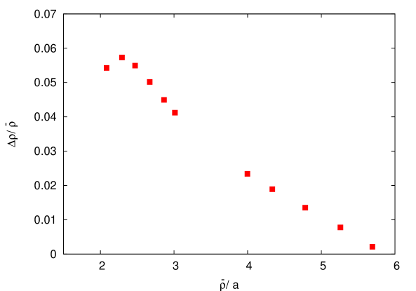
It is clear that the second procedure is non-local as opposed to the first one. This implies that in the case of noisy configurations the statistical fluctuations are reduced. On the contrary it fails when applied to an environment in which many instantons are present. That is the reason why we prefer to employ both methods instead of sticking to a single procedure. In any case, for instantons that are sufficiently smooth, the error in the size determination induced by the discretization remains at the few percent level. This is illustrated in figure 15 where we compare the size parameters, extracted from the two methods described above, for a set of twisted instanton configurations of varying sizes. For instantons larger than , the difference between the two determinations decreases as increases and remains in all cases below .
References
- [1] C. G. . Callan, R. F. Dashen and D. J. Gross, “Toward a theory of the strong interactions,” Phys. Rev. D 17 (1978) 2717.
- [2] G. ’t Hooft, “Computation of the quantum effects due to a four-dimensional pseudoparticle,” Phys. Rev. D 14 (1976) 3432 [Erratum-ibid. D 18 (1978) 2199].
- [3] A. A. Belavin and A. M. Polyakov, “Quantum Fluctuations Of Pseudoparticles,” Nucl. Phys. B 123 (1977) 429.
- [4] E. V. Shuryak, “The Role Of Instantons In Quantum Chromodynamics. 1. Physical Vacuum,” Nucl. Phys. B 203 (1982) 93; “The Role Of Instantons In Quantum Chromodynamics. 2. Hadronic Structure,” Nucl. Phys. B 203 (1982) 116; “The Role Of Instantons In Quantum Chromodynamics. 3. Quark - Gluon Nucl. Phys. B 203 (1982) 140.
- [5] E. M. Ilgenfritz and M. Muller-Preussker, “Statistical Mechanics Of The Interacting Yang-Mills Instanton Gas,” Nucl. Phys. B 184 (1981) 443.
- [6] D. Diakonov and V. Y. Petrov, “Instanton Based Vacuum From Feynman Variational Principle,” Nucl. Phys. B 245 (1984) 259.
- [7] T. Schafer, E. V. Shuryak, “Instantons in QCD,” Rev. Mod. Phys. 70, 323-426 (1998) [hep-ph/9610451].
- [8] M. F. Atiyah, N. J. Hitchin, V. G. Drinfeld, Y. .I. Manin, “Construction of Instantons,” Phys. Lett. A65, 185-187 (1978).
- [9] M. García Perez, A. González-Arroyo and P. Martínez, “From perturbation theory to confinement: How the string tension is built up,” Nucl. Phys. Proc. Suppl. 34 (1994) 228 [arXiv:hep-lat/9312066]. A. González-Arroyo and P. Martínez, “Investigating Yang-Mills theory and confinement as a function of the spatial volume,” Nucl. Phys. B 459 (1996) 337 [arXiv:hep-lat/9507001]. A. González-Arroyo, P. Martínez and A. Montero, “Gauge invariant structures and confinement,” Phys. Lett. B 359 (1995) 159 [arXiv:hep-lat/9507006]. A. González-Arroyo and A. Montero, “Do classical configurations produce Confinement?,” Phys. Lett. B 387 (1996) 823 [arXiv:hep-th/9604017].
- [10] R. S. Van de Water, “The CKM matrix and flavor physics from lattice QCD,” PoS LAT2009 (2009) 014 [arXiv:0911.3127 [hep-lat]].
- [11] M. Albanese et al. [APE Collaboration], “Glueball Masses and String Tension in Lattice QCD,” Phys. Lett. B 192 (1987) 163.
- [12] M. Falcioni, M. L. Paciello, G. Parisi and B. Taglienti, “Again On SU(3) Glueball Mass,” Nucl. Phys. B 251 (1985) 624.
- [13] T. A. DeGrand, A. Hasenfratz and T. G. Kovacs, “Topological structure in the SU(2) vacuum,” Nucl. Phys. B 505 (1997) 417 [arXiv:hep-lat/9705009].
- [14] A. Hasenfratz and C. Nieter, “Instanton content of the SU(3) vacuum,” Phys. Lett. B 439 (1998) 366 [arXiv:hep-lat/9806026].
- [15] C. Morningstar and M. J. Peardon, “Analytic smearing of SU(3) link variables in lattice QCD,” Phys. Rev. D 69 (2004) 054501 [arXiv:hep-lat/0311018].
- [16] M. Teper, “Instantons In The Quantized SU(2) Vacuum: A Lattice Monte Carlo Investigation,” Phys. Lett. B 162 (1985) 357.
- [17] B. Berg, “Dislocations And Topological Background In The Lattice O(3) Sigma Model,” Phys. Lett. B 104 (1981) 475.
- [18] J. Hoek, M. Teper and J. Waterhouse, “Topological Fluctuations And Susceptibility In SU(3) Lattice Gauge Theory,” Nucl. Phys. B 288 (1987) 589.
- [19] E. M. Ilgenfritz, M. L. Laursen, G. Schierholz, M. Muller-Preussker and H. Schiller, “First Evidence For The Existence Of Instantons In The Quantized SU(2) Lattice Vacuum,” Nucl. Phys. B 268 (1986) 693.
- [20] M. García Perez, A. González-Arroyo, J. R. Snippe and P. van Baal, “Instantons from over - improved cooling,” Nucl. Phys. B 413 (1994) 535 [arXiv:hep-lat/9309009].
- [21] P. de Forcrand, M. García Perez and I. O. Stamatescu, “Topology of the SU(2) vacuum: A lattice study using improved cooling,” Nucl. Phys. B 499 (1997) 409 [arXiv:hep-lat/9701012].
- [22] M. García Perez, O. Philipsen and I. O. Stamatescu, “Cooling, physical scales and topology,” Nucl. Phys. B 551 (1999) 293 [arXiv:hep-lat/9812006].
- [23] M. Luscher, “Properties and uses of the Wilson flow in lattice QCD,” JHEP 1008 (2010) 071 [arXiv:1006.4518 [hep-lat]].
- [24] S. J. Hands and M. Teper, “On The Value And Origin Of The Chiral Condensate In Quenched SU(2) Lattice Gauge Theory,” Nucl. Phys. B 347 (1990) 819.
- [25] T. A. DeGrand and A. Hasenfratz, “Low-lying fermion modes, topology and light hadrons in quenched QCD,” Phys. Rev. D 64 (2001) 034512 [arXiv:hep-lat/0012021].
- [26] R. G. Edwards, U. M. Heller and R. Narayanan, “The hermitian Wilson-Dirac operator in smooth SU(2) instanton backgrounds,” Nucl. Phys. B 522 (1998) 285 [arXiv:hep-lat/9801015].
- [27] P. Hasenfratz, V. Laliena and F. Niedermayer, “The index theorem in QCD with a finite cut-off,” Phys. Lett. B 427 (1998) 125 [arXiv:hep-lat/9801021].
- [28] F. Niedermayer, “Exact chiral symmetry, topological charge and related topics,” Nucl. Phys. Proc. Suppl. 73 (1999) 105 [arXiv:hep-lat/9810026].
- [29] I. Horvath, S. J. Dong, T. Draper, F. X. Lee, K. F. Liu, H. B. Thacker and J. B. Zhang, “On the local structure of topological charge fluctuations in QCD,” Phys. Rev. D 67 (2003) 011501 [arXiv:hep-lat/0203027].
- [30] C. Gattringer, “Testing the self-duality of topological lumps in SU(3) lattice gauge theory,” Phys. Rev. Lett. 88 (2002) 221601 [arXiv:hep-lat/0202002].
- [31] P. J. Moran, D. B. Leinweber and J. Zhang, “Wilson mass dependence of the overlap topological charge density,” Phys. Lett. B 695 (2011) 337 [arXiv:1007.0854 [hep-lat]].
- [32] F. Bruckmann and E. M. Ilgenfritz, “Laplacian modes probing gauge fields,” Phys. Rev. D 72 (2005) 114502 [arXiv:hep-lat/0509020].
- [33] S. Solbrig, F. Bruckmann, C. Gattringer, E. M. Ilgenfritz, M. Muller-Preussker and A. Schafer, “Smearing and filtering methods in lattice QCD - a quantitative comparison,” PoS LAT2007 (2007) 334 [arXiv:0710.0480 [hep-lat]].
- [34] F. Bruckmann, “Exploring the QCD vacuum - (some) recent developments in confinement and topology,” PoS LAT2007 (2007) 006 [arXiv:0710.2788 [hep-lat]].
- [35] F. Bruckmann, F. Gruber, C. B. Lang, M. Limmer, T. Maurer, A. Schafer and S. Solbrig, “Comparison of filtering methods in SU(3) lattice gauge theory,” PoS CONFINEMENT8 (2008) 045 [arXiv:0901.2286 [hep-lat]].
- [36] A. González-Arroyo and R. Kirchner, “Adjoint modes as probes of gauge field structure,” JHEP 0601 (2006) 029 [arXiv:hep-lat/0507036].
- [37] V. A. Novikov, M. A. Shifman, A. I. Vainshtein, V. I. Zakharov, “Supersymmetric Instanton Calculus (Gauge Theories with Matter),” Nucl. Phys. B260, 157-181 (1985).
- [38] H. Neuberger, “Exactly massless quarks on the lattice,” Phys. Lett. B 417 (1998) 141 [arXiv:hep-lat/9707022].
- [39] M. García Perez, A. González-Arroyo and A. Sastre, “Adjoint zero-modes as a tool to understand the Yang-Mills vacuum,” PoS LAT2007 (2007) 328 [arXiv:0710.0455 [hep-lat]];
- [40] M. García Perez, A. González-Arroyo and A. Sastre, “Probing the Yang-Mills vacuum with adjoint zero-modes,” PoS LATTICE2010 (2010) 285 [arXiv:1010.6210 [hep-lat]].
- [41] Alfonso Sastre. PhD Thesis: Application of the Dirac operator in the adjoint representation to Yang-Mills theories. September 2010, Universidad Autónoma de Madrid
- [42] S. Schaefer, R. Sommer and F. Virotta [ALPHA Collaboration], “Critical slowing down and error analysis in lattice QCD simulations,” Nucl. Phys. B 845 (2011) 93 [arXiv:1009.5228 [hep-lat]].
- [43] L. Del Debbio, H. Panagopoulos and E. Vicari, “Theta dependence of SU(N) gauge theories,” JHEP 0208 (2002) 044 [arXiv:hep-th/0204125].
- [44] B. Alles, G. Boyd, M. D’Elia, A. Di Giacomo and E. Vicari, “Hybrid Monte Carlo and topological modes of full QCD,” Phys. Lett. B 389 (1996) 107 [arXiv:hep-lat/9607049].
- [45] H. Neuberger, “A practical implementation of the overlap-Dirac operator,” Phys. Rev. Lett. 81 (1998) 4060 [arXiv:hep-lat/9806025].
- [46] R. G. Edwards, U. M. Heller and R. Narayanan, “A study of practical implementations of the overlap-Dirac operator in four dimensions,” Nucl. Phys. B 540, 457 (1999) [arXiv:hep-lat/9807017].
- [47] B. Jegerlehner, “Krylov space solvers for shifted linear systems,” arXiv:hep-lat/9612014.
- [48] H. Neuberger, “Minimizing storage in implementations of the overlap lattice-Dirac operator,” Int. J. Mod. Phys. C 10, 1051 (1999) [arXiv:hep-lat/9811019].
- [49] T. Kalkreuter and H. Simma, “An Accelerated Conjugate Gradient Algorithm To Compute Low Lying Eigenvalues: A Study For The Dirac Operator In SU(2) Lattice QCD,” Comput. Phys. Commun. 93 (1996) 33 [arXiv:hep-lat/9507023].
- [50] A. Borici, “On the Neuberger overlap operator,” Phys. Lett. B 453, 46 (1999) [arXiv:hep-lat/9810064].
- [51] T. C. Kraan and P. van Baal, “Exact T-duality between calorons and Taub - NUT spaces,” Phys. Lett. B 428 (1998) 268 [arXiv:hep-th/9802049]; “Periodic instantons with non-trivial holonomy,” Nucl. Phys. B 533 (1998) 627 [arXiv:hep-th/9805168]; “Monopole constituents inside SU(n) calorons,” Phys. Lett. B 435 (1998) 389 [arXiv:hep-th/9806034].
- [52] K. M. Lee, “Instantons and magnetic monopoles on R**3 x S(1) with arbitrary simple gauge groups,” Phys. Lett. B 426 (1998) 323 [arXiv:hep-th/9802012]; K. M. Lee and C. h. Lu, “SU(2) calorons and magnetic monopoles,” Phys. Rev. D 58, 025011 (1998) [arXiv:hep-th/9802108].
- [53] G. ’t Hooft, “Some Twisted Selfdual Solutions For The Yang-Mills Equations On A Hypertorus,” Commun. Math. Phys. 81 (1981) 267.
- [54] M. García Perez, A. González-Arroyo and B. Soderberg, “Minimum action solutions for SU(2) gauge theory on the torus with nonorthogonal twist,” Phys. Lett. B 235 (1990) 117; M. García Pérez and A. González-Arroyo, “Numerical study of Yang-Mills classical solutions on the twisted torus,” J. Phys. A 26 (1993) 2667 [arXiv:hep-lat/9206016].
- [55] G. ’t Hooft, “A Property Of Electric And Magnetic Flux In Nonabelian Gauge Theories,” Nucl. Phys. B 153 (1979) 141.
- [56] A. González-Arroyo, J. Jurkiewicz and C. P. Korthals-Altes, “Ground State Metamorphosis For Yang-Mills Fields On A Finite Periodic Lattice,” Published in Freiburg ASI 1981:0339 (QC175:N15).
- [57] A. Coste, A. Gonzalez-Arroyo, J. Jurkiewicz and C. P. Korthals Altes, Nucl. Phys. B 262 (1985) 67.
- [58] P. J. Braam and P. van Baal, “Nahm’s transformation for instantons,” Commun. Math. Phys. 122 (1989) 267.
- [59] D. Diakonov and V. Petrov, “Confining ensemble of dyons,” Phys. Rev. D 76 (2007) 056001 [arXiv:0704.3181 [hep-th]]; D. Diakonov, N. Gromov, V. Petrov and S. Slizovskiy, “Quantum weights of dyons and of instantons with non-trivial holonomy,” Phys. Rev. D 70 (2004) 036003 [arXiv:hep-th/0404042]; D. Diakonov, “Statistical physics of dyons and confinement,” Acta Phys. Polon. B 39 (2008) 3365 [arXiv:0807.0902 [hep-th]].
- [60] P. Gerhold, E. M. Ilgenfritz and M. Muller-Preussker, “An SU(2) KvBLL caloron gas model and confinement,” Nucl. Phys. B 760 (2007) 1 [arXiv:hep-ph/0607315]. a
- [61] F. Bruckmann, S. Dinter, E. M. Ilgenfritz, M. Muller-Preussker and M. Wagner, “Cautionary remarks on the moduli space metric for multi-dyon simulations,” Phys. Rev. D 79 (2009) 116007 [arXiv:0903.3075 [hep-ph]].