The New Physics sensitivity of the $s\rightarrow d\gamma$ transition and its accessibility through hadronic processes are thoroughly investigated. Firstly, the Standard Model predictions for the direct CP-violating observables in radiative $K$ decays are systematically improved. Besides, the magnetic contribution to $\varepsilon^{\prime}$ is estimated and found subleading, even in the presence of New Physics, and a new strategy to resolve its electroweak versus QCD penguin fraction is identified. Secondly, the signatures of a series of New Physics scenarios, characterized as model-independently as possible in terms of their underlying dynamics, are investigated by combining the information from all the FCNC transitions in the $s\rightarrow d$ sector.

 

Contents

1. 1 Introduction
2. 2 The flavor-changing electromagnetic currents
   1. 2.1 Long-distance effects
   2. 2.2 Phenomenological windows
3. 3 Standard Model predictions
   1. 3.1 $K\rightarrow\pi\pi\gamma$
   2. 3.2 $K_{L,S}\rightarrow\gamma\gamma$
   3. 3.3 Rare semileptonic decays
   4. 3.4 Virtual effects in $\varepsilon^{\prime}/\varepsilon$
4. 4 New Physics effects
   1. 4.1 Model-independent analysis
   2. 4.2 Tree-level FCNC
   3. 4.3 Loop-level FCNC
5. 5 Conclusions
6. A The $K\rightarrow\pi\pi\gamma$ decays in Chiral Perturbation Theory
   1. A.1 $\varepsilon_{+0\gamma}^{\prime}$ beyond $\mathcal{O}(p^{4})$
7. B Updated error analysis for $\mathcal{B}(K_{L}\rightarrow\pi^{0}\ell^{+}\ell^{-})$
8. References

 

1 Introduction

Quantum electrodynamics is among the most successful theories ever designed. At very low energy, up to a few MeV, its predictions have been tested and confirmed to a fantastic level of precision. At higher energies, with the advent of the Standard Model (SM) arises the possibility for the electromagnetic current to induce flavor transitions. This peculiar phenomenon requires a delicate interplay at the quantum level between the three families of matter particles. So delicate in fact that in the presence of physics beyond the Standard Model, significant deviations are expected. As for the past 150 years, electromagnetism could thus once more guide our quest for unification, and enlighten our understanding of Nature.

For this reason, the $b\rightarrow s\gamma$ and $\mu\rightarrow e\gamma$ transitions have received considerable attention. The former is known to NNLO precision in the SM [1], and has been measured accurately at the $B$ factories [2]. It is now one of the most constraining observables for New Physics (NP) models. The latter, obviously free of hadronic uncertainties, is so small in the SM that its experimental observation would immediately signal the presence of NP [3]. Further, most models do not suppress this transition as effectively as the SM, with rates within reach of the current MEG experiment at PSI [4].

The $s\rightarrow d\gamma$ process is complementary to $b\rightarrow s\gamma$ and $\mu\rightarrow e\gamma$, as the relative strengths of these transitions is a powerful tool to investigate the NP dynamics. However, two issues have severely hampered its abilities up to now. First, the $s\rightarrow d\gamma$ decay takes place deep within the QCD non-perturbative regime, and thus requires control over the low-energy hadronic physics. Second, these hadronic effects strongly enhance the SM contribution, to the point that identifying a possible deviation from NP is very challenging both theoretically and experimentally. To circumvent those difficulties is one of the goals of the present paper.

Indeed, the experimental situation calls for improved theoretical treatments. The recent experimental results [5] for the $K^{+}\rightarrow\pi^{+}\pi^{0}\gamma$ decay, driven by the $s\rightarrow d\gamma$ process, should be exploited. More importantly, several $K$ decay experiments will start in the next few years, NA62 at CERN, K0TO at J-Parc, and KLOE-II at the LNF. In view of their expected high luminosities, new strategies may open up to constrain, or even signal, the NP in the $s\rightarrow d\gamma$ transition. This requires identifying the most promising observables, both in terms of theoretical control over the SM contributions and in terms of sensitivity to NP effects. These are the two other goals of the paper.

In the next section, the anatomy of the $s\rightarrow d\gamma$ process in the SM is detailed, together with the tools required to deal with the long-distance QCD effects. From these general considerations, the best windows to probe the $s\rightarrow d\gamma$ decays are identified. These observables are then analyzed in details in the following section, where predictions for their SM contributions are obtained. Particular attention is paid to their sensitivity to short-distance effects, and thereby to possible NP contributions. This is put to use in the last (mostly self-contained) section, where the signatures of several NP scenarios are characterized in terms of correlations among the rare and radiative $K$ decays, as well as $\operatorname{Re}(\varepsilon^{\prime}/\varepsilon)$.

2 The flavor-changing electromagnetic currents

In the SM, the flavor changing electromagnetic current arises at the loop level, as depicted in Fig. 1. When QCD is turned off, and $m_{s,d}\ll m_{u,c,t}$, the single photon penguin can be embedded into local effective interactions of dimension greater than four:

$$\mathcal{H}_{eff}^{\gamma}=C_{\gamma}^{\pm}Q_{\gamma}^{\pm}+C_{\gamma^{\ast}}^{\pm}Q_{\gamma^{\ast}}^{\pm}+h.c.\;,$$ (1)

with the magnetic and electric operators defined as

$$Q_{\gamma}^{\pm}=\frac{Q_{d}e}{16\pi^{2}}\;(\bar{s}_{L}\sigma^{\mu\nu}d_{R}\pm\bar{s}_{R}\sigma^{\mu\nu}d_{L})\,F_{\mu\nu}\;,\;\;Q_{\gamma^{\ast}}^{\pm}=\frac{Q_{d}e}{16\pi^{2}}\;(\bar{s}_{L}\gamma^{\nu}d_{L}\pm\bar{s}_{R}\gamma^{\nu}d_{R})\,\partial^{\mu}F_{\mu\nu}\;,$$ (2)

and $2\sigma^{\mu\nu}=i[\gamma^{\mu},\gamma^{\nu}]$, $Q_{d}=-1/3$ the down-quark electric charge. For a real photon emission, $\partial^{\mu}F_{\mu\nu}=0$ so only the magnetic operators contribute. The corresponding Wilson coefficients are [6]

$$Q_{d}(C_{\gamma}^{+}-C_{\gamma}^{-})=\sqrt{2}G_{F}\lambda_{i}D_{0}^{\prime}\left(x_{i}\right)m_{s}\;,\;\;Q_{d}(C_{\gamma}^{+}+C_{\gamma}^{-})=\sqrt{2}G_{F}\lambda_{i}D_{0}^{\prime}\left(x_{i}\right)m_{d}\;,$$ (3)

and

$$Q_{d}(C_{\gamma^{\ast}}^{+}+C_{\gamma^{\ast}}^{-})=-2\sqrt{2}G_{F}\lambda_{i}D_{0}\left(x_{i}\right)\;,\;\;Q_{d}(C_{\gamma^{\ast}}^{+}-C_{\gamma^{\ast}}^{-})\approx 0\;,$$ (4)

where $i=u,c,t$, $\lambda_{i}=V_{is}^{\ast}V_{id}$ the CKM matrix elements, and $D_{0}^{(\prime)}(x_{i}\equiv m_{i}^{2}/M_{W}^{2})$ the loop functions (see e.g. Ref. [6] for their expressions). Summing over the three up-quark flavors, it is their dependences on the quark masses which ensure the necessary GIM breaking, since otherwise CKM unitarity $\lambda_{u}+\lambda_{c}+\lambda_{t}=0$ would force them to vanish. In this respect, $D_{0}^{\prime}(x)$ is suppressed for light quarks, while $D_{0}(x)$ breaks GIM logarithmically both for $x\rightarrow\infty$ and $x\rightarrow 0$. However, QCD corrections significantly soften the quadratic GIM breaking of $D_{0}^{\prime}(x)$ in the $x\rightarrow 0$ limit [7], and exacerbate the logarithmic one of $D_{0}(x)$ [8], making light-quark contributions significant for both operators.

Figure 1: The flavor-changing electromagnetic currents in the Standard Model.

In the presence of NP, new mechanisms could produce the $s\rightarrow d\gamma$ transition. Since the NP energy scale is presumably above the electroweak scale, these effects would simply enter into the Wilson coefficients of the same effective local operators (1). This is the shift we want to extract phenomenologically. In this respect, the magnetic operators are a priori most sensitive to NP for two reasons. First, the electric transition is essentially left-handed and the magnetic operators are very suppressed in the SM because right-handed external quarks $(s,d)_{R}$ are accompanied by the chiral suppression factor $m_{s,d}$. These strong suppressions may be lifted in the presence of NP, where larger chirality flip mechanisms can be available. Second, the magnetic operators are formally of dimension five, and thus a priori less suppressed by the NP energy scale than the dimension six electric operators. Sizeable NP effects could thus show up, as will be quantitatively analyzed in Sec. 4.

With the help of the standard QED interactions, the $\mathcal{H}_{eff}^{\gamma}$ operators also contribute to processes with more than one photon, where they compete with the effective operators directly involving several photon fields. For example, for two real photons, the dominant operators are

$$Q_{\gamma\gamma,||}^{\pm}=(\bar{s}_{L}d_{R}\pm\bar{s}_{R}d_{L})F_{\mu\nu}F^{\mu\nu},\;\;Q_{\gamma\gamma,\perp}^{\pm}=(\bar{s}_{L}d_{R}\pm\bar{s}_{R}d_{L})F_{\mu\nu}\tilde{F}^{\mu\nu}\;,$$ (5)

with $\tilde{F}^{\mu\nu}=\varepsilon^{\mu\nu\rho\sigma}F_{\rho\sigma}/2$. In the SM, the additional quark propagator in the two-photon penguin induces an $x^{-1}$ GIM breaking by the loop function (see Fig. 1$b$). Hence, the $c$ and $t$-quark contributions are completely negligible compared to the $u$-quark loop. Further, NP effects in these operators should be very suppressed since they are at least of dimension seven. So, whenever it contributes, the two photon penguin represents an irreducible long-distance SM background for the SD processes. The same is true for transitions with more than two photons, with the NP (up-quark loop) even more suppressed (enhanced), so those will not be considered here.

2.1 Long-distance effects

Once QCD is turned back on and with $m_{u}<m_{s,d}<m_{c,t}$, the $c$ and $t$ contributions remain local, but not the up quark loop. At the $K$ mass scale, the former are, together with possible NP, the short-distance (SD) contributions, and the latter are the SM-dominated long-distance (LD) contributions. Note that the SD contributions are also affected by long-distance effects, since phenomenologically, the matrix elements of the SD operators between low-energy meson states is needed.

Figure 2: Description of the radiative $K$ decays, starting with the electroweak scale interactions down to chiral perturbation theory, with illustrative examples of mesonic processes (the photons can be real or virtual). The green vertices arise from the currents in Eqs. (8, 9), the blue disks and square from the $\mathcal{O}(p^{2})$ weak Lagrangians Eq. (14) and $\mathcal{O}(p^{4})$ weak counterterms Eq. (16), respectively, and finally, the strong (black) and QED (red) vertices from Eq. (7).

To deal with these LD effects, the first step is to sum up the QCD-corrected interactions among the light quarks into an effective Hamiltonian [6]

$$\mathcal{H}_{eff}(\mu\approx 1\text{ GeV})=\sum_{\grave{\imath}=1}^{10}C_{i}\left(\mu\right)Q_{i}\left(\mu\right)+\mathcal{H}_{eff}^{\gamma}\left(\mu\right)+...\;,$$ (6)

with the four-quark current-current $(Q_{1,2})$, QCD penguin $(Q_{3,...,6})$, and electroweak penguin $(Q_{7,...,10})$ operators, and $\mathcal{H}_{eff}^{\gamma}\left(\mu\right)$ as in Eq. (1). Short-distance physics, including both the SM and NP effects, is encoded into the Wilson coefficients $C_{i}\left(\mu\right)$, see Fig. 2. The low-virtuality up, down, and strange quarks, i.e. the dynamics going on below the QCD perturbativity frontier $\mu\approx 1$ GeV, are dealt through the hadronic matrix elements of the effective operators.

At the hadronic scale, the strong dynamics is represented with chiral perturbation theory (ChPT), the effective theory for QCD with the pseudoscalar mesons as degrees of freedom [9]. At $\mathcal{O}(p^{2})$, the strong interaction Lagrangian is

$$\mathcal{L}_{strong}=\dfrac{F^{2}}{4}\langle D^{\mu}UD_{\mu}U^{\dagger}+\chi U^{\dagger}+U\chi^{\dagger}\rangle\;,$$ (7)

where $F=F_{\pi}\approx 92.4$ MeV, $U$ is a $3\times 3$ matrix function of the meson fields, $\chi=2B_{0}\operatorname*{diag}(m_{u},m_{d},m_{s})$ reproduces the explicit chiral symmetry breaking induced by the quark masses, and $\langle...\rangle$ means the flavor trace (we follow the notation of Ref. [10]). The covariant derivative includes external real or virtual photons, $D_{\mu}U=\partial_{\mu}U-ieA_{\mu}[U,Q]$, $Q=\operatorname*{diag}(2/3,-1/3,-1/3)$, as well as static $Z$ or $W$ currents coupled to leptonic states which do not concern us here.

To the strong Lagrangian (7), the electroweak operators of $\mathcal{H}_{eff}$ are added as effective interactions among the pseudoscalar mesons. So, the non-local, low-energy tails of the photon penguins of Fig. 1 are reconstructed using the effective hadronic representations of $Q_{1,...,10}$ to induce the weak transition, and the photon(s) emitted from light charged mesons occurring either as external particles (bremsstrahlung radiation) or inside loops (direct emission radiation), see Fig. 2. Note that the mesonic processes not only represent the $u$ quark loop in Fig. 1, but also $d$ and $s$ quark loops since the Fermi interaction is effectively replaced by the whole set of $Q_{1,...,10}$ operators at long-distance. So, let us construct the hadronic representations of $\mathcal{H}_{eff}$, starting with the electromagnetic operators.

2.1.1 Electromagnetic operators

The chiral realization of the $Q_{\gamma^{\ast}}^{\pm}$ operators requires that of the vector and axial-vector quark bilinears. At $\mathcal{O}(p^{2})$, these currents are related by the $SU(3)$ symmetry to the conserved electromagnetic current, and are thus entirely fixed from the Lagrangian (7):

$$\bar{q}_{L}^{I}\gamma^{\mu}q_{L}^{J}=i\frac{F^{2}}{2}(\partial^{\mu}U^{\dagger}U)^{JI},\;\;\;\;\bar{q}_{R}^{I}\gamma^{\mu}q_{R}^{J}=i\frac{F^{2}}{2}(\partial^{\mu}UU^{\dagger})^{JI}\;.$$ (8)

The $SU(3)$ breaking corrections start at $\mathcal{O}(p^{4})$ and are mild thanks to the Ademollo-Gatto theorem [11]. They can be precisely estimated from the charged current matrix elements, i.e. from $K_{\ell 3}$ decays. See Ref. [12] for a detailed analysis.

The chiral realization of the tensor currents in $Q_{\gamma}^{\pm}$ is more involved and starts at $\mathcal{O}(p^{4})$ since two derivatives are needed to get the correct Lorentz structure. Further, it cannot be entirely fixed but involves specific low-energy constants. By imposing charge conjugation and parity invariance (valid for QCD), the antisymmetry under $\mu\leftrightarrow\nu$, and the identity $i\varepsilon^{\alpha\beta\mu\nu}\sigma_{\mu\nu}=2\sigma^{\alpha\beta}\gamma_{5}$, only two free real parameters $a_{T}$ and $a_{T}^{\prime}$ remain (parts of these currents were given in Refs. [14, 13])

$$\bar{q}^{I}\sigma_{\mu\nu}P_{L}q^{J} =-i\frac{F^{2}}{2}a_{T}\left(D_{\mu}U^{\dagger}D_{\nu}UU^{\dagger}-D_{\nu}U^{\dagger}D_{\mu}UU^{\dagger}-i\varepsilon_{\mu\nu\rho\sigma}D^{\rho}U^{\dagger}D^{\sigma}UU^{\dagger}\right)^{JI}$$

$$\;\;\;\;+\frac{F^{2}}{2}a_{T}^{\prime}((F_{\mu\nu}^{L}-i\tilde{F}_{\mu\nu}^{L})U^{\dagger}+U^{\dagger}(F_{\mu\nu}^{R}-i\tilde{F}_{\mu\nu}^{R}))^{JI}\;\;,$$ (9a)

$$\bar{q}^{I}\sigma_{\mu\nu}P_{R}q^{J} =-i\frac{F^{2}}{2}a_{T}\left(D_{\mu}UD_{\nu}U^{\dagger}U-D_{\nu}UD_{\mu}U^{\dagger}U+i\varepsilon_{\mu\nu\rho\sigma}D^{\rho}UD^{\sigma}U^{\dagger}U\right)^{JI}$$

$$\;\;\;\;+\frac{F^{2}}{2}a_{T}^{\prime}(U(F_{\mu\nu}^{L}+i\tilde{F}_{\mu\nu}^{L})+(F_{\mu\nu}^{R}+i\tilde{F}_{\mu\nu}^{R})U)^{JI}\;.$$ (9b)

Numerically, we will use the lattice estimate [15]

$$B_{T}(2\;\text{GeV})=2m_{K}a_{T}=1.21(12)\;.$$ (10)

Being derived from a study of the $\langle\pi|\bar{s}\sigma_{\mu\nu}d|K\rangle$ matrix element, $SU(3)$ corrections are under control. A similar estimate of $B_{T}^{\prime}=2m_{K}a_{T}^{\prime}$ is not available yet. Instead, we can start from $\langle\gamma|\bar{u}\sigma_{\mu\nu}\gamma_{5}d|\pi^{-}\rangle$ and invoke the $SU(3)$ symmetry. Ref. [16], through a study of the $VT$ correlator, get $a_{T}^{\prime}=B_{0}/M_{V}^{2}$ and thus $B_{T}^{\prime}=2.7(5)$, assuming the standard ChPT sign conventions for the matrix elements. Another route is to use the magnetic susceptibility of the vacuum, $\langle 0|\bar{q}\sigma_{\mu\nu}q|0\rangle_{\gamma}$. From the lattice estimate in Ref. [17], we extract using $a_{T}^{\prime}=-\chi_{T}B_{0}/2$ the value $B_{T}^{\prime}(2$ GeV$)=2.67(17)$. Both techniques give similar results though their respective scales do not match. In addition, sizeable $SU(3)$ breaking effects cannot be ruled out since there is no Ademollo-Gatto protection for the tensor currents. So, to be conservative, we shall use

$$B_{T}^{\prime}(2\;\text{GeV})=2m_{K}a_{T}^{\prime}=3(1)\;.$$ (11)

At $\mathcal{O}(p^{4})$, the magnetic operators contribute to decay modes with at most two photons. With the chiral suppression expected for higher order terms, decays with three or more (real or virtual) photons should have a negligible sensitivity to $Q_{\gamma}^{\pm}$, hence are not included in our study.

In the SM, since the local operators sum up the short-distance part of the real photon penguins, the factor $m_{s,d}\sim\mathcal{O}(p^{2})$ in Eq. (3) are not included in the bosonization. Instead, they are kept as perturbative parameters in the Wilson coefficients $C_{\gamma}^{\pm}$, to be evaluated at the same scale as the form factors $B_{T}$ and $B_{T}^{\prime}$. Numerically, to account for the large QCD corrections, the Wilson coefficient of the magnetic operator in $b\rightarrow s\gamma$ can be used for $\operatorname{Im}C_{\gamma}^{\pm}$, since the CKM elements for the $u$, $c$, and $t$ contributions scale similarly. With $m_{s}(2$ GeV$)=101_{-21}^{+29}$ MeV [18] and $C_{7\gamma}(2$ GeV$)\approx-0.36$ from Ref. [6], we shall use

$$\frac{\operatorname{Im}C_{\gamma}^{\pm}(2\;\text{GeV})_{\text{SM}}}{G_{F}m_{K}}=\mp\sqrt{2}\frac{C_{7\gamma}(2\,\text{GeV)}}{Q_{d}}\frac{m_{s}(2\;\text{GeV})}{m_{K}}\operatorname{Im}\lambda_{t}=\mp 0.31(8)\times\operatorname{Im}\lambda_{t}\;,$$ (12)

to be compared to $\mp 0.17\operatorname{Im}\lambda_{t}$ with only the top quark. In view of the large error on $m_{s}$, the LO approximation is adequate. For $\operatorname{Re}C_{\gamma}^{\pm}$, contrary to the situation in $b\rightarrow s\gamma$, the top quark is strongly suppressed as $\operatorname{Re}\lambda_{c}\approx-\operatorname{Re}\lambda_{u}\gg\operatorname{Re}\lambda_{t}$. With the light quarks further enhanced by QCD corrections, an estimate is delicate. Naively rescaling the above result gives

$$\frac{\operatorname{Re}C_{\gamma}^{\pm}(2\;\text{GeV})_{\text{SM}}}{G_{F}m_{K}}\approx\frac{\operatorname{Re}\lambda_{c}}{\operatorname{Im}\lambda_{c}}\times\frac{\operatorname{Im}C_{\gamma}^{\pm}(2\;\text{GeV})_{\text{SM}}}{G_{F}m_{K}}\approx\mp 0.06\;.$$ (13)

Evidently, one should not take this as more than a rough estimate of the order of magnitude of the $c$ quark and high-virtuality $u$ quark contributions. In any case, we will be mostly concern by CP-violating observables in the following, so will not use Eq. (13).

2.1.2 Four-quark weak operators

By matching their chiral structures, the four-quark weak current-current and penguin operators are represented at $\mathcal{O}(p^{2})$ as [19]

$$\mathcal{L}_{8} =F^{4}G_{8}\langle\lambda_{6}L_{\mu}L^{\mu}\rangle\;,\;\;$$ (14a)

$$\mathcal{L}_{27} =\frac{F^{4}}{18}G_{27}^{1/2}\left(\langle\lambda_{1}L_{\mu}\rangle\langle\lambda_{4}L^{\mu}\rangle+\langle\lambda_{2}L_{\mu}\rangle\langle\lambda_{5}L^{\mu}\rangle-10\langle\lambda_{6}L_{\mu}\rangle\langle\lambda_{3}L^{\mu}\rangle+18\langle\lambda_{6}L_{\mu}\rangle\langle QL^{\mu}\rangle\right)$$

$$\;\;\;\;+\frac{5F^{4}}{18}G_{27}^{3/2}\left(\langle\lambda_{1}L_{\mu}\rangle\langle\lambda_{4}L^{\mu}\rangle+\langle\lambda_{2}L_{\mu}\rangle\langle\lambda_{5}L^{\mu}\rangle+2\langle\lambda_{6}L_{\mu}\rangle\langle\lambda_{3}L^{\mu}\rangle\right)\;,$$ (14b)

$$\mathcal{L}_{ew} =F^{6}e^{2}G_{ew}\langle\lambda_{6}U^{\dagger}QU\rangle\;,$$ (14c)

where $L^{\mu}\equiv U^{\dagger}D^{\mu}U$, $\lambda_{i}$ are the Gell-Mann matrices, and $G_{27}\equiv G_{27}^{3/2}=G_{27}^{1/2}$ in the isospin limit. If QCD was perturbative down to the hadronic scale, the low-energy constants could be computed from the Wilson coefficients at that scale as

$$\{C_{1}-C_{2},C_{3-6},C_{9},C_{10}\}\rightarrow G_{8}\;\;,\;\;\;\{C_{1}+C_{2},C_{9},C_{10}\}\rightarrow G_{27}\;\;,\;\;\;\{C_{7},C_{8}\}\rightarrow G_{ew}\;.$$ (15)

The ChPT scale is too low for this to be possible however. Instead, the low-energy constants are fixed from experiment, especially from $K\rightarrow\pi\pi$. The consequence is that neither the $\Delta I=1/2$ rule, embodied in their real parts as $\operatorname{Re}G_{27}/\operatorname{Re}G_{8}\equiv\omega=1/22.4$, nor the direct CP-violation parameters like $\varepsilon^{\prime}$ generated from their imaginary parts, can be precisely computed from first principles.

At tree level, if $\mathcal{L}_{8}$, $\mathcal{L}_{27}$, or $\mathcal{L}_{ew}$ contribute to a radiative decay, it is only through bremsstrahlung amplitudes [22, 20, 21]. The dynamics is therefore trivial at $\mathcal{O}(p^{2})$ because Low’s theorem [23] shows that such emissions are entirely fixed in terms of the non-radiative $K\rightarrow 2\pi,3\pi$ amplitudes. Thus, the non-trivial dynamics corresponding to the low-energy tails of the photon penguins arise at $\mathcal{O}(p^{4})$, where they are represented in terms of non-local meson loops, as well as additional $\mathcal{O}(p^{4})$ local effective interactions, in particular the $\Delta I=1/2$ enhanced $N_{14},...,N_{18}$ octet counterterms [24, 25]:

$$\mathcal{L}_{8}^{\text{CT}}=-i\langle\lambda_{6}(N_{14}\{f_{+}^{\mu\nu},L_{\mu}L_{\nu}\}+N_{15}L_{\mu}f_{+}^{\mu\nu}L_{\nu}+N_{16}\{f_{-}^{\mu\nu},L_{\mu}L_{\nu}\}+N_{17}L_{\mu}f_{-}^{\mu\nu}L_{\nu}+iN_{18}(f_{+\mu\nu}^{2}-f_{-\mu\nu}^{2}))\rangle\;,$$ (16)

with $f_{\pm}^{\mu\nu}\equiv F_{L}^{\mu\nu}\pm U^{\dagger}F_{R}^{\mu\nu}U$, and $F_{L}^{\mu\nu}=F_{R}^{\mu\nu}=-eQF^{\mu\nu}$ for external photons. There are also counterterms relevant for the renormalization of the non-radiative $K\rightarrow n\pi$ amplitudes occurring in the bremsstrahlung contributions, for the strong structure of the $\pi^{+}\pi^{-}\gamma^{\ast}$ or $K^{+}K^{-}\gamma^{\ast}$ vertices, and for the odd-parity sector (proportional to $\varepsilon$ tensors) which will not concern us here. Note that the need to compute the $Q_{1,...,10}$ contributions at $\mathcal{O}(p^{4})$ also follows from the chiral representation (9) of the magnetic operators starting at that order.

The structure of the effective interactions (16) is dictated by the chiral counting rules and the chiral symmetry properties of the underlying weak operators, but the (renormalized) $N_{i}$ constants cannot be computed from first principles and have to be fixed experimentally, exactly like the $\mathcal{O}(p^{2})$ constants $G_{8,27,ew}$ of Eq. (14).

2.1.3 The hadronic tails of the photon penguins

The set of interactions included within ChPT is complete, in the sense that all the possible effective interactions with the required symmetries are present at a given order. So, it may appear that at $O(p^{4})$, once the weak interactions (14) are added to the strong dynamics (7), and including the counterterms (16), there is no more need to separately include the SD electromagnetic operators through Eq. (8) and (9). All their effects would be accounted for in the values of the low-energy constants. Indeed, these constants should sum up the physics taking place above the mesonic scale, i.e. the hadronic degrees of freedom just above the octet of pseudoscalar mesons [25, 26] as well as the quark and gluon degrees of freedom above the GeV scale [27].

This actually holds for $Q_{\gamma^{\ast}}^{\pm}$, but not for $Q_{\gamma}^{\pm}$. Indeed, only the former have the same chiral structures as the $N_{i}$ counterterms. Whenever $Q_{\gamma^{\ast}}^{\pm}$ contribute, so do the $N_{i}$, but $Q_{\gamma}^{\pm}$ can contribute to many modes where the $N_{i}$ are absent (see Table 1 in the next section) and must therefore appear explicitly in the effective theory. Including the $\Delta I=3/2$ suppressed $\mathcal{L}_{27}^{\text{CT}}$ [24, 28] or the $e^{2}$-suppressed $\mathcal{L}_{ew}^{\text{CT}}$ [29] counterterms would not change this picture, so for simplicity we consider only $\mathcal{L}_{8}^{\text{CT}}$.

This mismatch between $\mathcal{L}_{8}^{\text{CT}}$ and $Q_{\gamma}^{\pm}$ has an important dynamical implication since the weak counterterms reflect the chiral structures of the meson loops built on the $Q_{1,...,10}$ operators (14) at $\mathcal{O}(p^{4})$. While these meson loops can genuinely represent the low-energy tail of the virtual photon penguin, i.e. the $\log(x_{u})$ singularity of the $D_{0}(x)$ function, they never match the chiral representation of $Q_{\gamma}^{\pm}$. The meson dynamics lacks the required $m_{s,d}$ chirality flip at $\mathcal{O}(p^{4})$, relying instead on the long-distance dynamics, i.e. momenta. One can understand this phenomenon as the low-energy equivalent of the known importance of the $Q_{2}^{c}=(\bar{s}c)_{V-A}\otimes(\bar{c}b)_{V-A}$ contribution to $b\rightarrow s\gamma$ [7]. Clearly, $s\rightarrow d\gamma$ has to be even more affected than $b\rightarrow s\gamma$ by QCD corrections since the photon is never hard ($q_{\gamma}^{2}<m_{K}^{2}$), and an inclusive analysis is not possible. So for $s\rightarrow d\gamma$, the $Q_{2}^{u}=(\bar{s}u)_{V-A}\otimes(\bar{u}d)_{V-A}$ contribution, represented through $Q_{1,...,10}$, corresponds to a whole class of purely long-distance processes, often including IR divergent bremsstrahlung radiations. They are not suppressed at all, contrary to the naive expectation from $D_{0}^{\prime}(x)\rightarrow x$ as $x\rightarrow 0$, but instead dominate most of the radiative processes.

With this in mind, we can understand at least qualitatively another striking feature of all the radiative modes where $Q_{\gamma^{\ast}}^{\pm}$ is absent. The meson loops are always finite at $\mathcal{O}(p^{4})$, except for $K_{1}\rightarrow\pi^{+}\pi^{-}\pi^{0}\gamma(\gamma)$ [22]. This means that not only the SD part of the magnetic operators decouples, but also to some extent the intermediate QCD degrees of freedom (i.e., the resonances). By contrast, the $N_{i}$ combinations occurring for the modes induced by $Q_{\gamma^{\ast}}^{\pm}$ are always scale dependent, somewhat reminiscent of the factorization of the low-energy part of the virtual photon penguin. So, the behavior of the flavor-changing electromagnetic current is not very different from that of the flavor-conserving one. In that case, being protected by the QED gauge symmetry, the form-factor for $\langle\gamma(q)|\pi^{+}\pi^{-}\rangle$ or $\langle\gamma(q)|K^{+}K^{-}\rangle$ is not renormalized at all at $q^{2}=0$, while vector resonances saturate the off-shell behavior [25, 26].

From these observations, we can reasonably expect that whenever a finite combination of $N_{i}$ occurs for a process with only real photons, it should be significantly suppressed. Indeed, not only the divergences cancel among the $N_{i}$, but also the large $Q_{\gamma^{\ast}}^{\pm}$ contribution embedded into them (this was already noted using large $N_{c}$ arguments in Ref. [32]), as well as the resonance effects describing the purely strong structure of the photon. As our analysis of $K^{+}\rightarrow\pi^{+}\pi^{0}\gamma$ in Sec. 3 will show, this suppression is supported by the recent experimental data, see Eq. (26).

2.2 Phenomenological windows

The $K$ decay channels where the electromagnetic operators contribute are listed in Table 1, together with their CP signatures. For the electric operators, at least one of the photons needs to be virtual, i.e. coupled to a Dalitz pair $\ell^{+}\ell^{-}$. In this respect, remark that all the electromagnetic operators produce the $\ell^{+}\ell^{-}$ pair in the same $1^{--}$ state, so the electric and magnetic operators can only be disentangled using real photon decays.

		$\perp$	$||$			$M$	$E$	$L$
$K_{2}\rightarrow\gamma\gamma$	$a_{T}^{\prime}$	$\operatorname{Re}C_{\gamma}^{+}$	$\operatorname{Im}C_{\gamma}^{-}$	–
$K_{2}\rightarrow\pi^{0}\gamma\gamma$	$a_{T}^{\prime}$	$\operatorname{Im}C_{\gamma}^{-}$	$\operatorname{Re}C_{\gamma}^{+}$	$K_{2}\rightarrow\pi^{0}\gamma$	$a_{T}$	–	–	$\operatorname{Im}C_{\gamma^{(\ast)}}^{+}$
$K^{+}\rightarrow\pi^{+}\gamma\gamma$	$3a_{T}+a_{T}^{\prime}$	$C_{\gamma}^{-}$	$C_{\gamma}^{+}$	$K^{+}\rightarrow\pi^{+}\gamma$	$a_{T}$	–	–	$C_{\gamma^{(\ast)}}^{+}$
$K_{2}\rightarrow\pi^{0}\pi^{0}\gamma\gamma$	$a_{T}^{\prime}$	$\operatorname{Re}C_{\gamma}^{+}$	$\operatorname{Im}C_{\gamma}^{-}$	$K_{2}\rightarrow\pi^{0}\pi^{0}\gamma$	$a_{T}$	–	–	$\operatorname{Re}C_{\gamma^{(\ast)}}^{-}$
$K_{2}\rightarrow\pi^{+}\pi^{-}\gamma\gamma$	$a_{T},a_{T}^{\prime}$	$\operatorname{Re}C_{\gamma}^{+}$	$\operatorname{Im}C_{\gamma}^{-}$	$K_{2}\rightarrow\pi^{+}\pi^{-}\gamma$	$a_{T}$	$\operatorname{Re}C_{\gamma}^{+}$	$\operatorname{Im}C_{\gamma}^{-}$	$\operatorname{Re}C_{\gamma^{(\ast)}}^{-}$
$K^{+}\rightarrow\pi^{+}\pi^{0}\gamma\gamma$	$a_{T},a_{T}^{\prime}$	$C_{\gamma}^{+}$	$C_{\gamma}^{-}$	$K^{+}\rightarrow\pi^{+}\pi^{0}\gamma$	$a_{T}$	$C_{\gamma}^{+}$	$C_{\gamma}^{-}$	$C_{\gamma^{(\ast)}}^{-}$
$K_{2}\rightarrow 3\pi^{0}\gamma\gamma$	$a_{T}^{\prime}$	$\operatorname{Im}C_{\gamma}^{-}$	$\operatorname{Re}C_{\gamma}^{+}$	$K_{2}\rightarrow 3\pi^{0}\gamma$	$a_{T}$	–	–	$\operatorname{Im}C_{\gamma^{(\ast)}}^{+}$

Table 1: Dominant processes where the electromagnetic operators contribute, omitting the $K\rightarrow(n\pi)\gamma^{\ast}\gamma^{(\ast)}$, $n\geq 0$ decays. The $K_{1}\approx K_{S}$ processes are obtained from $K_{2}\approx K_{L}$ by inverting real and imaginary parts. The symbol $\perp$ ($||$) means the photon pair in an odd (even) parity state, i.e. a $F_{\mu\nu}\tilde{F}^{\mu\nu}$ ($F_{\mu\nu}F^{\mu\nu}$) coupling, and similarly, $M$ ($E$) means odd (even) parity magnetic (electric) emissions. For $\pi\pi$ modes, the lowest multipole is understood (i.e., $\pi\pi$ in a $S$ wave for $\gamma\gamma$ modes, and a $P$ wave for $\gamma$ modes). The last column denotes longitudinal off-shell photon emissions, proportional to $q^{2}g^{\alpha\beta}-q^{\alpha}q^{\beta}$ with $q$ the photon momentum, for which the $Q_{\gamma^{\ast}}^{\pm}$ operators also enters. The $K\rightarrow 3\pi\gamma(\gamma)$ decays with charged pions are not included since dominated by bremsstrahlung radiations off $K\rightarrow 3\pi$ [22]. Finally, $a_{T}$ and $a_{T}^{\prime}$ are the low-energy constants entering the tensor current (9).

For most of the decays in Table 1, the LD contributions are dominant, obscuring the SD parts where NP could be evidenced. The situation is thus very different than in $b\rightarrow s\gamma$, where the $u$ quark contribution is suppressed by $V_{ub}\ll 1$. However, in $K$ physics, the long-distance contributions are essentially CP-conserving. Indeed, CP-violation from the four-quark operators is known to be small from $\operatorname{Re}(\varepsilon^{\prime}/\varepsilon)^{\exp}$. In the SM, this follows from the CKM scalings $\operatorname{Re}\lambda_{u}\gg\operatorname{Re}\lambda_{t}\sim\operatorname{Im}\lambda_{t}$ and $\operatorname{Im}\lambda_{u}=0$. So, for CP-violating observables, one recovers a situation reminiscent of $b\rightarrow s\gamma$, with the dominant SM contributions arising from the charm and top quarks, both of similar size a priori. Only for such observables can we hope that the interesting short-distance physics in $Q_{\gamma}^{\pm}$ and $Q_{\gamma^{\ast}}^{\pm}$ emerges from the long-distance SM background.

All the decays in Table 1 have a CP-conserving contribution, and thus in most cases the best available CP-violating observables are CP-asymmetries. Since they arise from CP-odd interferences between the various decay mechanisms, the dominant CP-conserving processes must be under sufficiently good theoretical control. In addition, these CP-asymmetries being usually small, the decay rates should be sufficiently large, and not completely dominated by bremsstrahlung radiations. Indeed, even though these radiations are under excellent theoretical control thanks to Low’s theorem [23], they would render the short-distance physics too difficult to access experimentally.

Imposing these conditions on the modes in Table 1, the best windows for the electromagnetic operators are:

• Real photons: Since the branching ratios decrease as the number of pions increases, the best candidates to constrain $Q_{\gamma}^{\pm}$ are the $K_{L,S}\rightarrow\gamma\gamma$ decays for two real photons and the $K\rightarrow\pi\pi\gamma$ decays for a single real photon. All the other modes with real photons are either significantly more suppressed (see e.g. Ref. [20, 14] for a study of $K\rightarrow\pi\gamma\gamma$), or dominated by bremsstrahlung contributions. By contrast, these radiations are suppressed for $K_{L}\rightarrow\pi^{+}\pi^{-}\gamma$ since $K_{L}\rightarrow\pi^{+}\pi^{-}$ is CP-violating, and for $K^{+}\rightarrow\pi^{+}\pi^{0}\gamma$ thanks to the $\Delta I=1/2$ rule. The relevant CP-violating asymmetries are those either between $K_{L}-K_{S}$ decay amplitudes, between $K^{+}-K^{-}$ differential decay rates, or in some phase-space variables. This latter possibility usually requires some additional information on the photon polarization, accessible e.g. through Dalitz pairs. But besides the significant suppression of the total rates, this brings in the electric operators, making the analysis much more involved, so these observables will not be considered here (see e.g. Ref. [33]).

• Virtual photons: The best candidates to probe the electric operators are the $K_{L}\rightarrow\pi^{0}\ell^{+}\ell^{-}$ ($\ell=e,\mu$) decays, for which $K_{L}\rightarrow\pi^{0}\gamma^{\ast}[\rightarrow\ell^{+}\ell^{-}]$ is CP-violating hence free of the up-quark contribution (see e.g. Ref. [34]). As detailed in Sec. 3.3 (see Fig. 6), there are nevertheless an indirect CP-violating piece from the small $\varepsilon K_{2}$ component of the $K_{L}$ as well as a CP-conserving contribution from the four-quark operators with two intermediate photons, but these are suppressed and under control [35, 36]. The direct CP-asymmetry in $K^{\pm}\rightarrow\pi^{\pm}\ell^{+}\ell^{-}$ is not competitive because of its small $\sim 10^{-9}$ branching ratio, and of the hadronic uncertainties in the long-distance contributions [8, 37].
  With $K_{L}\rightarrow\pi^{0}\ell^{+}\ell^{-}$ sensitive to $Q_{\gamma^{\ast}}^{+}$, information on $Q_{\gamma^{\ast}}^{-}$ would also be needed to disentangle the left and right-handed currents. But since $\langle\gamma|Q_{\gamma^{\ast}}^{-}|K^{0}(q)\rangle\sim q^{\nu}q^{\mu}F_{\mu\nu}=0$, and with $K\rightarrow\pi\gamma^{\ast}\gamma$ sensitive again to $Q_{\gamma^{\ast}}^{+}$, the simplest observables are the $K\rightarrow\pi\pi\gamma^{\ast}$ and $K\rightarrow\pi\pi\gamma^{\ast}\gamma^{(\ast)}$ modes, which are suppressed and dominated by LD contributions. For the time being, we will thus concentrate only on $Q_{\gamma^{\ast}}^{+}$.

In summary, the best windows to probe for the electromagnetic operators are the CP-asymmetries in the $K_{L,S}\rightarrow\gamma\gamma$, $K_{L,S}\rightarrow\pi^{+}\pi^{-}\gamma$, and $K^{+}\rightarrow\pi^{+}\pi^{0}\gamma$ decays, and the $K_{L}\rightarrow\pi^{0}\ell^{+}\ell^{-}$ decay rates. For completeness, it should be mentioned that the magnetic operators also contributes to radiative hyperon decays [38] or to the $B_{s}\rightarrow B_{d}^{\ast}\gamma$ transition [39], which will not be analyzed here.

3 Standard Model predictions

In order to get clear signals of NP, the SM contributions have to be under good theoretical control. We rely on the available OPE analyses for the Wilson coefficients in the SM [6], and concentrate on the remaining long-distance parts of these contributions. For CP-violating observables, they originate either indirectly from the hadronic penguins $Q_{3}\rightarrow Q_{10}$ or directly from the magnetic operators $Q_{\gamma}^{\pm}$. Since the former indirect contributions are suppressed, while the $C_{\gamma}^{\pm}$ are very small in the SM, both often end up being comparable. These LD contributions have to be estimated in ChPT. This is rather immediate for $Q_{\gamma}^{\pm}$ given the hadronic representations (9), but significantly more involved for the hadronic penguins, requiring a detailed analysis of the meson dynamics relevant for each process. In addition, some free low-energy constants necessarily enter, which have to be fixed from other observables.

Thus, the goal of this section is threefold. First, the observables relevant for the study of $Q_{\gamma}^{\pm}$ are presented. This includes the $K\rightarrow\pi\pi\gamma$ rate and CP-asymmetries, the $K_{L,S}\rightarrow\gamma\gamma$ direct CP-violation parameters, the rare semileptonic decays $K\rightarrow\pi\ell^{+}\ell^{-}$, and finally, the hadronic parameter $\varepsilon^{\prime}$. Second, the hadronic penguin contributions to the radiative decay observables are brought under control by relating them to well-measured parameters like $\varepsilon^{\prime}$. In doing this, special care is paid on the possible impacts of NP in $Q_{3}\rightarrow Q_{10}$, which have to be separately parametrized. This is crucial to confidently extract the contributions from $Q_{\gamma}^{\pm}$, where NP could also be present. This constitutes the third goal of the section: To establish the master formulas for all the observables relevant in the study of $Q_{\gamma}^{\pm}$, which will form the basis of the NP analysis of the next section.

3.1 $K\rightarrow\pi\pi\gamma$

From Lorentz and gauge invariance, the general decomposition of the $K\left(P\right)\rightarrow\pi_{1}\left(K_{1}\right)\pi_{2}\left(K_{2}\right)\gamma\left(q\right)$ amplitude is [40, 41, 42]

$$\mathcal{M}\left(K\rightarrow\pi_{1}\pi_{2}\gamma\right)=\left[E\left(z_{i}\right)\frac{K_{2}^{\mu}K_{1}\cdot q-K_{1}^{\mu}K_{2}\cdot q}{m_{K}^{3}}+M\left(z_{i}\right)\frac{i\varepsilon^{\mu\nu\rho\sigma}K_{1,\nu}K_{2,\rho}q_{\sigma}}{m_{K}^{3}}\right]\varepsilon_{\mu}^{\ast}(q)\;.$$ (17)

The reduced kinematical variables $z_{1,2}=K_{1,2}\cdot q/m_{K}^{2}$ are related to the energies of the two pions which we identify as $\pi_{1}\pi_{2}=\pi^{+}\pi^{-}$, $\pi^{0}\pi^{0}$, or $\pi^{+}\pi^{0}$, and $z_{3}=z_{1}+z_{2}=E_{\gamma}/m_{K}$ is the photon energy in the $K$ rest-frame.

The two terms $E\left(z_{i}\right)$ and $M\left(z_{i}\right)$ are respectively the (dimensionless) electric and magnetic amplitudes [43], and do not interfere in the rate once summed over the photon polarizations. The electric part can be further split into a bremsstrahlung and a direct emission term:

$$E(z_{1},z_{2})=E_{IB}(z_{1},z_{2})+E_{DE}(z_{1},z_{2})\;,$$ (18)

while the magnetic part is a pure direct emission, $M\equiv M_{DE}$. When the photon energy goes to zero, only $E_{IB}$ is divergent and, according to Low’s theorem [23], entirely fixed from the non-radiative process $K\rightarrow\pi_{1}\pi_{2}$.

The direct emission terms $E_{DE}$ and $M_{DE}$ are constant in that limit. In addition, they can be expanded in multipoles, according to the angular momentum of the two pions [44]:

$$E_{DE}(z_{1},z_{2})e^{i\delta_{DE}}=E_{1}(z_{3})e^{i\delta_{1}}+E_{2}(z_{3})e^{i\delta_{2}}(z_{1}-z_{2})+E_{3}(z_{3})e^{i\delta_{3}}(z_{1}-z_{2})^{2}+...\;,$$ (19)

and similarly for $M_{DE}$. There are several interesting features in this expansion [10]: (1) for $K^{0}$ decays, the odd and even multipoles produce the $\pi\pi$ pair in opposite CP states (2) when CP-conserving, the dipole emission $E_{1}$ dominates over higher multipoles which have to overcome the angular momentum barrier ($|z_{1}-z_{2}|<0.2$), (3) the strong phases can be assigned consistently to each multipole since it produces the $\pi\pi$ state in a given angular momentum state, (4) the magnetic operators $Q_{\gamma}^{-(+)}$ contributes to the electric (magnetic) dipole emission amplitudes when $\pi_{1}\pi_{2}=\pi^{+}\pi^{0}$ or $\pi^{+}\pi^{-}$, and (5) the $E_{IB}$ and $E_{DE}$ amplitudes interfere and have different weak and strong phases, hence generate a CP-asymmetry for both the neutral $K^{0}\rightarrow\pi^{+}\pi^{-}\gamma$ and charged $K^{+}\rightarrow\pi^{+}\pi^{0}\gamma$ modes. That is how we plan to extract the $Q_{\gamma}^{-}$ contribution, so let us analyze each decay in turn.

3.1.1 $K^{+}\rightarrow\pi^{+}\pi^{0}\gamma$

For the $K^{+}\rightarrow\pi^{+}\pi^{0}\gamma$ decay, instead of $z_{1,2}$, the standard phase-space variables are chosen as the $\pi^{+}$ kinetic energy $T_{c}^{\ast}$ and $W^{2}\equiv(q\cdot P)(q\cdot K_{1})/m_{\pi^{+}}^{2}m_{K}^{2}$ [44]. Indeed, pulling out the bremsstrahlung contribution, the differential rate can be written

$$\frac{\partial^{2}\Gamma}{\partial T_{c}^{\ast}\partial W^{2}}=\frac{\partial^{2}\Gamma_{IB}}{\partial T_{c}^{\ast}\partial W^{2}}\left(1-2\frac{m_{\pi^{+}}^{2}}{m_{K}}\operatorname{Re}\left(\frac{E_{DE}}{eA_{IB}}\right)W^{2}+\frac{m_{\pi^{+}}^{4}}{m_{K}^{2}}\left(\left|\frac{E_{DE}}{eA_{IB}}\right|^{2}+\left|\frac{M_{DE}}{eA_{IB}}\right|^{2}\right)W^{4}\right)\;,$$ (20)

where $A_{IB}=A\left(K^{+}\rightarrow\pi^{+}\pi^{0}\right)$ is constant but both $E_{DE}$ and $M_{DE}$ are functions of $W^{2}$ and $T_{c}^{\ast}$. The main interest of $K^{+}\rightarrow\pi^{+}\pi^{0}\gamma$ is clearly apparent: $A_{IB}$ is pure $\Delta I=3/2$ hence suppressed, making the direct emission amplitudes easier to access. Note that the strong phase of $A_{IB}$ is that of the $\pi\pi$ rescattering in the $I=2$, $L=0$ state, as confirmed by a full $\mathcal{O}(p^{4})$ computation. This is not trivial a priori since both Watson’s and Low’s theorem deal with asymptotic states. Actually, Low’s theorem takes place after Watson’s theorem, in agreement with the naive expectation from the relative strength of QED and strong interactions.

Total and differential rates:

Given its smallness, we can assume the absence of CP-violation when discussing these observables. Experimentally, the electric and magnetic amplitudes (taken as constant) have been fitted in the range $T_{c}^{\ast}\leq 80$ MeV and $0.2<W<0.9$ by NA48/2 [5]. Using their parametrization,

$$X_{E} =\frac{-\operatorname{Re}\left(E_{DE}/eA_{IB}\right)}{m_{K}^{3}\cos(\delta_{1}^{1}-\delta_{0}^{2})}=\left(-24\pm 4\pm 4\right)\;\text{GeV}^{-4}\;,\;$$ (21a)

$$X_{M} =\frac{\left|M_{DE}/eA_{IB}\right|}{m_{K}^{3}}=\left(254\pm 6\pm 6\right)\;\text{GeV}^{-4}\;,$$ (21b)

with $\delta_{J}^{I}$ the strong $\pi\pi$ rescattering phase in the isospin $I$ and angular momentum $J$ state. The magnetic amplitude is dominated by the QED anomaly and will not concern us here (see e.g. Refs. [31, 45]). For the electric amplitude, we obtain at $\mathcal{O}(p^{4})$:

$$X_{E}=\frac{3G_{8}/G_{27}}{40\pi^{2}F_{\pi}^{2}m_{K}^{2}}\frac{\cos(\delta_{DE}-\delta_{0}^{2})}{\cos(\delta_{1}^{1}-\delta_{0}^{2})}\left[E^{loop}(W^{2},T_{c}^{\ast})-\dfrac{m_{K}^{2}\operatorname{Re}\bar{N}}{m_{K}^{2}-m_{\pi}^{2}}\right]\;,$$ (22)

with the expression of $E^{loop}$ given in Appendix A. The $\bar{N}$ term contains both the $\mathcal{L}_{8}^{\text{CT}}$ counterterms [40] and the $Q_{\gamma}^{-}$ contributions

$$\operatorname{Re}\bar{N}\equiv(4\pi)^{2}\operatorname{Re}(N_{14}-N_{15}-N_{16}-N_{17})-\frac{2G_{F}}{3G_{8}}B_{T}\frac{\operatorname{Re}C_{\gamma}^{-}}{G_{F}m_{K}}\;,$$ (23)

when $27$-plet counterterms are neglected (or rather parametrically included into the $N_{i}$, together with higher order momentum-independent chiral corrections). To a good approximation, the loop contribution $E^{loop}(W^{2},T_{c}^{\ast})$ is dominated by the leading multipole $E_{1}^{loop}(z_{3})$, in which case $\delta_{DE}=\delta_{1}^{1}$. Note that $E_{1}^{loop}(z_{3})$ is still a function of the photon energy, hence indirectly of $W^{2}$ and $T_{c}^{\ast}$.

Figure 3: Basic topologies for the $K\rightarrow\pi\pi\gamma$ loops, with the vertices colored according to the conventions of Fig. 2. The photon is to be attached in all possible ways. However, in accordance with Low’s theorem, most of these diagrams renormalize the $\mathcal{O}(p^{2})$ bremsstrahlung process, leaving only genuine substracted three-point loops (thus involving at least one charged meson) for the direct emission amplitudes. The transition is $\Delta I=1/2$ ($3/2$) when the weak vertex is $K^{+}\pi^{-}\eta$ or $K^{0}\pi^{+}\pi^{-}$ ($K^{+}\pi^{-}\pi^{0}$). The counterterms and $Q_{\gamma}^{-}$ contribute only to $K^{+}\rightarrow\pi^{+}\pi^{0}\gamma$ and $K^{0}\rightarrow\pi^{+}\pi^{-}\gamma$.

In our computation of $E_{1}^{loop}$, we include both the $\mathcal{L}_{8}$ and $\mathcal{L}_{27}$ contributions. Indeed, as shown in Fig. 3, the large $\pi\pi$ loop occurs only for the $\Delta I=3/2$ channel, making it competitive with the $\Delta I=1/2$ contributions arising entirely from the small $\pi K$ and $\eta K$ loops. As a result, we find $E_{1}^{loop}(0)=-0.25$, to be compared to $-0.16$ in Ref. [42]. In addition, the $\pi\pi$ loop generates a significant slope. Though this momentum dependence over the experimental phase-space is mild, these cuts are far from the $z_{3}=0$ point, resulting in a further enhancement. Indeed, over the experimental range (but not outside of it), $E_{1}^{loop}$ is well described by

$$\left[E_{1}^{loop}(W,T_{c}^{\ast})\right]_{T_{c}^{\ast}\leq 80MeV,0.2<W<0.9}\approx-0.260-0.051W+0.089\frac{T_{c}^{\ast}}{m_{K}}\;.$$ (24)

Since experimentally, no slope were included, we average $E_{1}^{loop}$ over the experimental range (using the $dT_{c}^{\ast}dW$ measure to match the binning procedure of Ref. [5]), and find

$$\left\langle E_{1}^{loop}(W,T_{c}^{\ast})\right\rangle_{T_{c}^{\ast}\leq 80MeV,0.2<W<0.9}=-0.280\;\;\rightarrow\;X_{E}^{loop}=-17.6\;GeV^{-4}\;.$$ (25)

Note that we checked that in the presence of the slopes as predicted at $\mathcal{O}(p^{4})$ that the fitted values of $X_{E}$ and $X_{M}$ are not altered significantly.

Once $E_{1}^{loop}$ is known, we can constrain the local term $\bar{N}$ using the experimental measurement of $X_{E}$:

$$\operatorname{Re}\bar{N}=0.095\pm 0.083\;.$$ (26)

This is much smaller than the $\mathcal{O}(1)$ expected for the $N_{i}$ on dimensional grounds or from factorization [40], but confirms the picture described in Sec. 2.1.3. Evidently, so long as the $N_{i}$ are not better known, we cannot get an unambiguous bound on $\operatorname{Re}C_{\gamma}^{-}$. Still, barring a large fortuitous cancellation,

$$\frac{|\operatorname{Re}C_{\gamma}^{-}|}{G_{F}m_{K}}\lesssim 0.1\;.$$ (27)

Note that this bound is rather close to our naive estimate (13) of the charm-quark contribution to the real photon penguin in the SM.

Direct CP-violating asymmetries:

CP-violation in $K^{+}\rightarrow\pi^{+}\pi^{0}\gamma$ is quantified by the parameter $\varepsilon_{+0\gamma}^{\prime}$, defined from

$$\operatorname{Re}\left(\frac{E_{DE}}{eA_{IB}}\right)\left(K^{\pm}\rightarrow\pi^{\pm}\pi^{0}\gamma\right)\approx\frac{\operatorname{Re}E_{DE}}{e\operatorname{Re}A_{IB}}\left[\cos(\delta_{DE}-\delta_{0}^{2})\mp\sin(\delta_{DE}-\delta_{0}^{2})\varepsilon_{+0\gamma}^{\prime}\right]\;,$$ (28)

as [10]

$$\varepsilon_{+0\gamma}^{\prime}\equiv\frac{\operatorname{Im}E_{DE}}{\operatorname{Re}E_{DE}}-\frac{\operatorname{Im}A_{IB}}{\operatorname{Re}A_{IB}}\;.$$ (29)

To reach this form, we use the fact that both $\operatorname{Im}E_{DE}$ and $\operatorname{Im}A_{IB}$ change sign under $CP$, but not the strong phase $\delta_{DE}$ and $\delta_{0}^{2}$, and work to first order in $\operatorname{Im}A_{IB}/\operatorname{Re}A_{IB}$. Since $E_{2}$ has the same strong phase as $A_{IB}$, and higher multipoles are completely negligible, we can replace $E_{DE}$ by the dipole emission $E_{1}$ to an excellent approximation, so that $\delta_{DE}=\delta_{1}^{1}$.

Plugging Eq. (28) in Eq. (20), we get the differential asymmetry, which can be integrated over phase-space according to various definitions. Still, no matter the choice, these phase-space integrations tend to strongly suppress the overall sensitivity to $\varepsilon_{+0\gamma}^{\prime}$ since the rate is dominantly CP-conserving [10]. For example, NA48/2 [5] use the partially integrated asymmetry

$$a_{CP}(W^{2})=\frac{\partial\Gamma^{+}/\partial W^{2}-\partial\Gamma^{-}/\partial W^{2}}{\partial\Gamma^{+}/\partial W^{2}+\partial\Gamma^{-}/\partial W^{2}}=\frac{-2m_{\pi^{+}}^{2}m_{K}^{2}X_{E}W^{2}\;\sin(\delta_{DE}-\delta_{0}^{2})\;\varepsilon_{+0\gamma}^{\prime}}{1+2m_{\pi^{+}}^{2}m_{K}^{2}X_{E}W^{2}+m_{\pi^{+}}^{4}m_{K}^{4}(\left|X_{E}\right|^{2}+\left|X_{M}\right|^{2})W^{4}}\;,$$ (30)

where the dependences of $X_{E}$ and $X_{M}$ on $T_{c}^{\ast}$ are dropped, which is a reasonable approximation within the considered phase-space. Given the experimental values for $X_{E}$ and $X_{M}$, and combined with $\sin(\delta_{1}^{1}-\delta_{0}^{2})\approx\sin(7^{\circ})\approx 0.12$ [5, 46], $a_{CP}(W^{2})\lesssim 0.01\varepsilon_{+0\gamma}^{\prime}$ over the whole $W^{2}$ range. Clearly, integrating over $W^{2}$ to get the total rate charge asymmetry (or the induced direct CP-asymmetry in $K^{\pm}\rightarrow\pi^{\pm}\pi^{0}$ [47]) would suppress the sensitivity even more. Because of this, the current bound is rather weak [5]

$$\sin(\delta_{DE}-\delta_{2})\varepsilon_{+0\gamma}^{\prime}=\left(-2.5\pm 4.2\right)\times 10^{-2}\;.$$ (31)

Actually, thanks to the fact that $X_{E}<0$, there is an alternative observable which is not phase-space suppressed. Defining $\partial^{2}\Gamma_{DE}^{\pm}=\partial^{2}\Gamma^{\pm}-\partial^{2}\Gamma_{IB}^{\pm}$, and integrating over $T_{c}^{\ast}$, the direct emission differential rates $\partial\Gamma_{DE}^{+}/\partial W^{2}$ and $\partial\Gamma_{DE}^{-}/\partial W^{2}$ vanish at slightly different values of $W^{2}$, so we can construct the asymmetry,

$$a_{CP}^{0}=\frac{W_{\partial\Gamma_{DE}^{+}/\partial W^{2}=0}^{2}-W_{\partial\Gamma_{DE}^{-}/\partial W^{2}=0}^{2}}{W_{\partial\Gamma_{DE}^{+}/\partial W^{2}=0}^{2}+W_{\partial\Gamma_{DE}^{-}/\partial W^{2}=0}^{2}}=-\tan(\delta_{DE}-\delta_{2})\varepsilon_{+0\gamma}^{\prime}\;.$$ (32)

The zeros are around $W^{2}\approx 0.16$, i.e. within the experimental range $0.2<W<0.9$. Of course, it remains to be seen whether the experimental precision needed to perform significant fits to the zeros of $\partial\Gamma_{DE}^{\pm}/\partial W^{2}$ is not prohibitive.

Let us analyze the prediction for $\varepsilon_{+0\gamma}^{\prime}$ in the SM. At $\mathcal{O}(p^{4})$, discarding for now the counterterms and the electromagnetic operators, we obtain (see Appendix A)

$$\varepsilon_{+0\gamma}^{\prime}(z_{3})=\frac{\sqrt{2}|\varepsilon^{\prime}|}{\omega}f(z_{3},\Omega)\;,\;\;f(z_{3},\Omega)=\frac{-1}{1+\omega h_{20}(z_{3})}-\frac{\Omega}{1-\Omega}\frac{\omega\delta h_{20}(z_{3})}{1+\omega h_{20}(z_{3})}\;,$$ (33)

where $\omega=1/22.4$, $h_{20}(z_{3})$ is the ratio of the $G_{27}$ and $G_{8}$ loop functions, enhanced by the $\pi\pi$ contributions to the former, while $\delta h_{20}(z_{3})$ is the ratio of the $G_{ew}$ and $G_{8}$ loop functions and is $\mathcal{O}(1)$. The parameter $\Omega$ is defined as

$$\frac{\operatorname{Im}A_{2}}{\operatorname{Im}A_{0}}\equiv\omega\Omega\;.$$ (34)

It represents the fraction of electroweak versus QCD penguins in $\varepsilon^{\prime}$,

$$\varepsilon^{\prime}=i\frac{e^{i(\delta_{0}^{2}-\delta_{0}^{0})}}{\sqrt{2}}\omega\left(\frac{\operatorname{Im}A_{2}}{\operatorname{Re}A_{2}}-\frac{\operatorname{Im}A_{0}}{\operatorname{Re}A_{0}}\right)=i\frac{e^{i(\delta_{0}^{2}-\delta_{0}^{0})}}{\sqrt{2}}\frac{\operatorname{Im}A_{0}}{\operatorname{Re}A_{0}}\omega(\Omega-1)\;.$$ (35)

As shown in Fig. 4, a conservative range is $\Omega\in[-1,+0.8]$. Values between $[+0.2,+0.5]$ are favored by current analyses in the SM, but large NP cannot be ruled out.

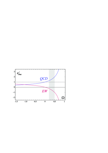
Figure 4: Fractions of QCD and electroweak penguins in $\varepsilon^{\prime}$. The absence of electroweak penguins corresponds to $\Omega=0$. Destructive interference occurs for values between $0$ and $1$ (with a singularity at $1$ since it corresponds to a complete cancellation between both types of penguins). Current analyses in the SM favor a limited destructive interference, i.e. $\Omega\in[+0.2,+0.5]$ (see e.g. Ref. [48, 50, 49]).

A crucial observation is that $\varepsilon_{+0\gamma}^{\prime}$ is rather insensitive to $\Omega$, because $\omega\delta h_{20}(z_{3})$ is suppressed by $\omega$, so that $f(z_{3},\Omega)\approx-2/3$. Varying $\Omega$ in the large range $[-1,+0.8]$, as well as including the potential impact of the $\mathcal{L}_{8}^{\text{CT}}$ counterterms (subject to the constraint Eq. (26)) does not affect $\varepsilon_{+0\gamma}^{\prime}$ much (see Appendix A), and we conservatively obtain

$$\varepsilon_{+0\gamma}^{\prime}(Q_{3,...,10})=-0.55(25)\times\frac{\sqrt{2}|\varepsilon^{\prime}|}{\omega}=-0.64(31)\times 10^{-4}\;,$$ (36)

using $\operatorname{Re}(\varepsilon^{\prime}/\varepsilon)^{\exp}=(1.65\pm 26)\times 10^{-3}$ [18]. The slight growth of $\varepsilon_{+0\gamma}^{\prime}$ with $z_{3}$ is negligible compared to its error. Since it is based on the experimental value of $|\varepsilon^{\prime}|$, and given the large range allowed for $\Omega$, this estimate is valid even in the presence of NP in the four-quark operators.

The stability of this prediction actually means that even a precise measurement of $\varepsilon_{+0\gamma}^{\prime}$ would not help to understand the physical content of $\varepsilon^{\prime}$, which would require measuring $\Omega$. On the other hand, it may help to unambiguously distinguish a contribution from $Q_{\gamma}^{-}$,

$$\varepsilon_{+0\gamma}^{\prime}(Q_{\gamma}^{-})=\frac{\operatorname{Im}E_{DE}(Q_{\gamma}^{-})}{\operatorname{Re}E_{DE}}=\frac{B_{T}}{20\pi^{2}}\frac{G_{F}/G_{27}}{F_{\pi}^{2}(m_{K}^{2}-m_{\pi}^{2})X_{E}}\frac{\operatorname{Im}C_{\gamma}^{-}}{G_{F}m_{K}}=+2.8(7)\frac{\operatorname{Im}C_{\gamma}^{-}}{G_{F}m_{K}}\;,$$ (37)

where we used the experimental determination (21) of $\operatorname{Re}E_{DE}$. So, the magnetic operator is competitive with the four-quark operators already in the SM, where we find from Eq. (12),

$$\varepsilon_{+0\gamma}^{\prime}(Q_{\gamma}^{-})|_{\text{SM}}=+1.2(4)\times 10^{-4}\;.$$ (38)

Hence, summing Eq. (36) and (38), there is a significant cancellation at play and $\varepsilon_{+0\gamma}^{\prime}|_{\text{SM}}=0.5(5)\times 10^{-4}$. This is still far below the current bound on $\varepsilon_{+0\gamma}^{\prime}$ derived from Eq. (31), which translates as

$$\frac{\operatorname{Im}C_{\gamma}^{-}}{G_{F}m_{K}}=-0.08\pm 0.13\;,$$ (39)

thus leaving ample room for NP effects.

3.1.2 $K_{L}\rightarrow\pi^{+}\pi^{-}\gamma$

For this mode, the large $\pi\pi$ loop is present in both the $\Delta I=1/2$ and $\Delta I=3/2$ channel, see Fig. 3, so including the latter does not change the picture for the total rate. On the other hand, the situation for the CP-violating parameter $\bar{\varepsilon}_{+-\gamma}^{\prime}$, defined from [10]

$$\bar{\varepsilon}_{+-\gamma}^{\prime}\equiv\eta_{+-\gamma}-\eta_{+-}\;,\;\;\eta_{+-\gamma}\equiv\frac{A(K_{L}\rightarrow\pi^{+}\pi^{-}\gamma)_{E_{IB}+E_{1}}}{A(K_{S}\rightarrow\pi^{+}\pi^{-}\gamma)_{E_{IB}+E_{1}}}\;,\;\;\eta_{+-}\equiv\frac{A(K_{L}\rightarrow\pi^{+}\pi^{-})}{A(K_{S}\rightarrow\pi^{+}\pi^{-})}\;,$$ (40)

is altered significantly. The restriction to the dipole terms originates in their dominance in the $K_{S}$ decay. The parameter $\eta_{+-\gamma}$ is then purely CP-violating since the $K_{L}\rightarrow\pi^{+}\pi^{-}\gamma$ dipole emissions violate CP. The direct dipole emission amplitudes $E_{1}^{L,S}$ for $K_{L,S}\rightarrow\pi^{+}\pi^{-}\gamma$ are functions of the photon energy $z_{3}$ only, and can be written as

$$E_{1}^{S}=\operatorname{Re}E_{+-}\;,\;\;E_{1}^{L}=i\operatorname{Im}E_{+-}+\bar{\varepsilon}\operatorname{Re}E_{+-}\;.$$ (41)

Parametrizing the CP-violating IB amplitude as $E_{IB}^{L}=\eta_{+-}E_{IB}^{S}$, including the strong phases but working to leading order in $\omega$ and in the CP-violating quantities [10],

$$\bar{\varepsilon}_{+-\gamma}^{\prime}=e^{i(\delta_{1}^{1}-\delta_{0}^{0})}\frac{m_{K}z_{1}z_{2}}{e\sqrt{2}}\frac{\operatorname{Re}E_{+-}}{\operatorname{Re}A_{0}}\left(\varepsilon^{\prime}+i\left(\frac{\operatorname{Im}A_{0}}{\operatorname{Re}A_{0}}-\frac{\operatorname{Im}E_{+-}}{\operatorname{Re}E_{+-}}\right)\right)\;.$$ (42)

As stated in Ref. [10], $\bar{\varepsilon}_{+-\gamma}^{\prime}$ is a measure of direct CP-violation. The $z_{1}z_{2}$ momentum dependence comes from the bremsstrahlung amplitude $E_{IB}^{S}$, which we write in terms of the $K\rightarrow\pi\pi$ isospin amplitudes using $A(K_{S}\rightarrow\pi^{+}\pi^{-})=\sqrt{2}A_{0}+A_{2}$. Over the $K^{0}\rightarrow\pi^{+}\pi^{-}\gamma$ phase-space, $z_{1}z_{2}$ is the largest when $E_{\gamma}^{\ast}$ is at its maximum (and the bremsstrahlung at its minimum), but always strongly suppresses the asymmetry since $z_{1}z_{2}\lesssim 0.030$. Following Ref. [51], to avoid dragging along this phase-space factor, we define the direct CP-violating parameter $\varepsilon_{+-\gamma}^{\prime}$

$$\varepsilon_{+-\gamma}^{\prime}\equiv\frac{\bar{\varepsilon}_{+-\gamma}^{\prime}}{z_{1}z_{2}}=\frac{\eta_{+-\gamma}-\eta_{+-}}{z_{1}z_{2}}\;.$$ (43)

Experimentally, this parameter has been studied indirectly through the time-dependence observed in the $\pi^{+}\pi^{-}\gamma$ decay channel [52] (using material in the beam to regenerate $K_{S}$ states), which is sensitive to the interference between the $K_{L}\rightarrow\pi^{+}\pi^{-}\gamma$ and $K_{S}\rightarrow\pi^{+}\pi^{-}\gamma$ decay amplitudes. Importantly, the experimental parameter $\eta_{+-\gamma}$ used in Ref. [52] (also quoted by the PDG [18]) is not the same as the one in Eq. (40) but requires additional phase-space integrations. Following Ref. [51] to pull these out, the experimental measurement $\tilde{\eta}_{+-\gamma}=(2.35\pm 0.07)\times 10^{-3}$ translates as

$$|\varepsilon_{+-\gamma}^{\prime}|<0.06\;.$$ (44)

The $E_{+-}$ amplitude can be predicted at $\mathcal{O}(p^{4})$ in ChPT, with the result (neglecting the counterterms and electromagnetic operators for now)

$$\frac{\operatorname{Im}E_{+-}}{\operatorname{Re}E_{+-}}=\frac{\operatorname{Im}A_{0}}{\operatorname{Re}A_{0}}\frac{1+\omega\Omega(h_{20}^{\prime}(z_{3})+\delta h_{20}^{\prime}(z_{3}))}{1+\omega h_{20}^{\prime}(z_{3})}\;,$$ (45)

where $\Omega$ is defined in Eq. (34), and $h_{20}^{\prime}(z_{3})$, $\delta h_{20}^{\prime}(z_{3})$ are ratios of loop functions (see Appendix A). Because the $\pi\pi$ loop is allowed in the $\Delta I=1/2$ channel, $h_{20}^{\prime}(z_{3})\approx 1/\sqrt{2}\ll\omega^{-1}$ while $\delta h_{20}^{\prime}(z_{3})$ is tiny and can be safely neglected. Plugging this in $\varepsilon_{+-\gamma}^{\prime}$, the sensitivity to $\Omega$ disappears completely

$$\varepsilon_{+-\gamma}^{\prime}(Q_{3,...,10})=ie^{i(\delta_{1}^{1}-\delta_{0}^{0})}\frac{m_{K}}{e\sqrt{2}}\frac{\operatorname{Re}E_{+-}}{\operatorname{Re}A_{0}}|\varepsilon^{\prime}|\left(e^{i(\delta_{0}^{2}-\delta_{0}^{0})}-1\right)\;.$$ (46)

As for $\varepsilon_{+0\gamma}^{\prime}$, there is no way to learn something about $\varepsilon^{\prime}$ by measuring $\varepsilon_{+-\gamma}^{\prime}$. Also, remark that $\varepsilon_{+-\gamma}^{\prime}$ is suppressed by the $\Delta I=1/2$ rule through its proportionality to $|\varepsilon^{\prime}|$, contrary to $\varepsilon_{+0\gamma}^{\prime}$ in Eq. (36).

The same combination of counterterms occur for $K^{0}\rightarrow\pi^{+}\pi^{-}\gamma$ and $K^{+}\rightarrow\pi^{+}\pi^{0}\gamma$. The bound in Eq. (26) shows that this combination is of the order of the $\pi K$ and $\eta K$ loops, which are much smaller than the $\pi\pi$ loop. So, they can be safely neglected and we finally predict

$$\varepsilon_{+-\gamma}^{\prime}(Q_{3,...,10})\approx\dfrac{m_{K}^{2}}{(4\pi F_{\pi})^{2}}h_{0}(z_{3}/2)\times|\varepsilon^{\prime}|\times e^{-i\pi/3}=-1.5(5)\times 10^{-6}\times e^{-i\pi/3}\;,$$ (47)

with $h_{0}(z_{3}/2)\approx-4\sqrt{2}\operatorname{Re}h_{\pi\pi}\left(-z_{3}\right)\approx-2.2$, $\delta_{0}^{2}-\delta_{0}^{0}\approx-45^{\circ}$, and $\delta_{1}^{1}-\delta_{0}^{2}\approx 7^{\circ}$. We conservatively add by hand a 30% error to account for the chiral corrections to the loop functions. This result is an order of magnitude below the bound derived in Ref. [10] because having kept track of the $G_{8}$, $G_{27}$, and $G_{ew}$ contributions, we could prove that $\varepsilon_{+-\gamma}^{\prime}(Q_{3,...,10})$ is suppressed by the $\Delta I=1/2$ rule. As for $\varepsilon_{+0\gamma}^{\prime}$, this estimate is valid even in the presence of NP in the four-quark operators since it is independent of $\Omega$ and takes $\operatorname{Re}(\varepsilon^{\prime}/\varepsilon)^{\exp}$ as input.

With $\varepsilon_{+-\gamma}^{\prime}(Q_{3,...,10})$ extremely suppressed, $\varepsilon_{+-\gamma}^{\prime}$ becomes sensitive to the presence of the $Q_{\gamma}^{-}$ operator, even in the SM. Its impact on $E_{DE}^{S}$ is negligible given the bound (27) but $E_{DE}^{L}$ receives an extra contribution (see Appendix A), so that

$$\varepsilon_{+-\gamma}^{\prime}(Q_{\gamma}^{-})=\frac{-G_{F}/G_{8}}{6(2\pi)^{2}}B_{T}\frac{m_{K}^{4}}{F_{\pi}^{2}(m_{K}^{2}-m_{\pi}^{2})}\frac{\operatorname{Im}C_{\gamma}^{-}}{G_{F}m_{K}}e^{i\phi_{\gamma}}\approx 0.2\frac{\operatorname{Im}C_{\gamma}^{-}}{G_{F}m_{K}}e^{i\phi_{\gamma}}\;,$$ (48)

with $\phi_{\gamma}\equiv\delta_{1}^{1}-\delta_{0}^{0}+\pi/2\approx 52^{\circ}$ and $G_{8}<0$ in our conventions. With the SM value (12) for $\operatorname{Im}C_{\gamma}^{-}$, this gives

$$\varepsilon_{+-\gamma}^{\prime}(Q_{\gamma}^{-})_{\text{SM}}=+8(3)\times 10^{-6}\times e^{i\phi_{\gamma}}\;,$$ (49)

which is about five times larger than $\varepsilon_{+-\gamma}^{\prime}(Q_{3,...,10})$, but still very small compared to $\varepsilon_{+0\gamma}^{\prime}$. The current measurement (44) requires

$$\frac{|\operatorname{Im}C_{\gamma}^{-}|}{G_{F}m_{K}}<0.3\;,$$ (50)

which is slightly looser than the bound (39) obtained from the direct CP-asymmetry in $K^{+}\rightarrow\pi^{+}\pi^{0}\gamma$.

3.2 $K_{L,S}\rightarrow\gamma\gamma$

CP-violating asymmetries for $K\rightarrow\gamma\gamma$ can be defined through the parameters (adopting the notation of Ref. [10])

$$\eta_{\gamma\gamma}^{\perp}=\frac{A(K_{S}\rightarrow(\gamma\gamma)_{\perp})}{A(K_{L}\rightarrow(\gamma\gamma)_{\perp})}=\varepsilon+\varepsilon_{\perp}^{\prime}\;,\;\;\eta_{\gamma\gamma}^{||}=\frac{A(K_{L}\rightarrow(\gamma\gamma)_{||})}{A(K_{S}\rightarrow(\gamma\gamma)_{||})}=\varepsilon+\varepsilon_{||}^{\prime}\;.$$ (51)

Experimentally, these CP-violating parameters could be accessed through time-dependent interference experiments, i.e. with $K^{0}$ or $\bar{K}^{0}$ beams [53], so the photon polarization need not be measured using the suppressed decays with Dalitz pairs.

Let us parametrize the $K^{0}\rightarrow\gamma(k_{1},\mu)\gamma(k_{2},\nu)$ amplitudes as

$$A(K^{0} \rightarrow(\gamma\gamma)_{||})=\frac{1}{\sqrt{2}}A_{\gamma\gamma}^{||}\times(\alpha G_{F}m_{K})\times(k_{1}^{\nu}k_{2}^{\mu}-k_{1}\cdot k_{2}g^{\mu\nu})\;,$$ (52a)

$$A(K^{0} \rightarrow(\gamma\gamma)_{\perp})=\frac{1}{\sqrt{2}}A_{\gamma\gamma}^{\perp}\times(\alpha G_{F}m_{K})\times i\varepsilon^{\mu\nu\rho\sigma}k_{1,\rho}k_{2\sigma}\;,\;\;$$ (52b)

so that the direct CP-violating parameters are expressed as

$$\varepsilon_{||,\perp}^{\prime}=i\left(\frac{\operatorname{Im}A_{\gamma\gamma}^{||,\perp}}{\operatorname{Re}A_{\gamma\gamma}^{||,\perp}}-\frac{\operatorname{Im}A_{0}}{\operatorname{Re}A_{0}}\right)\;.$$ (53)

We can fix $|A_{\gamma\gamma}^{||}|=0.133(4)$ and $|A_{\gamma\gamma}^{\perp}|=0.0800(3)$ from the $K_{L,S}\rightarrow\gamma\gamma$ decay rates [18], which are dominantly CP-conserving. In ChPT, $A_{\gamma\gamma}^{||}$ originates from a $\pi^{+}\pi^{-}$ loop and $A_{\gamma\gamma}^{\perp}$ is induced by the $\pi^{0}$, $\eta$, $\eta^{\prime}$ meson poles together with the QED anomaly, see Fig. 5.

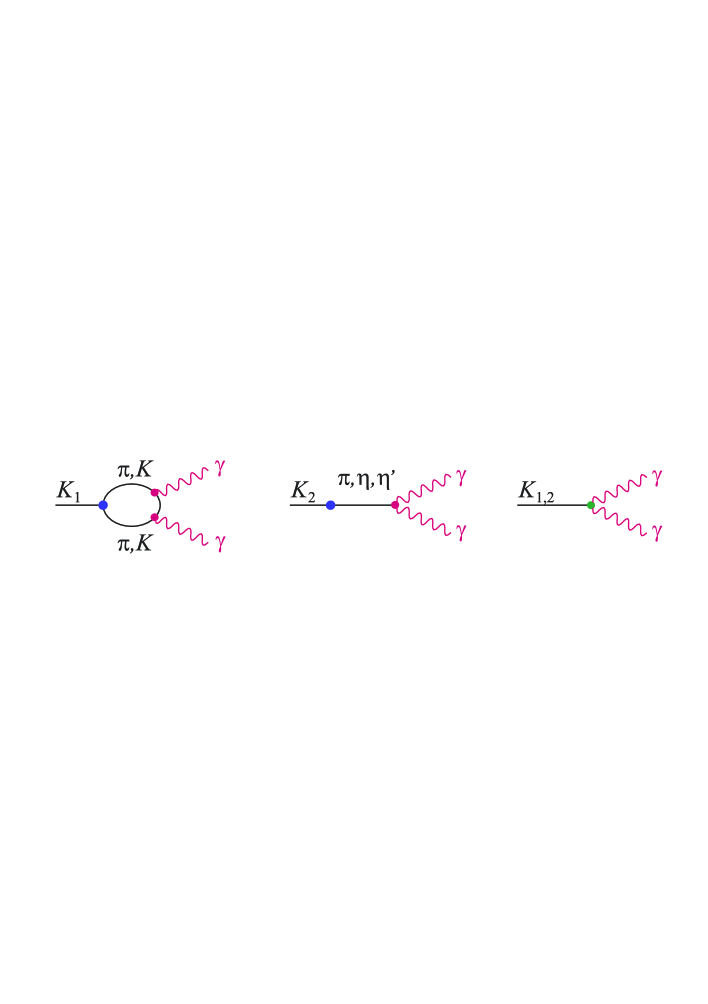
Figure 5: The transition $K\rightarrow\gamma\gamma$ in the SM, with the vertices colored according to the conventions of Fig. 2. The meson loop produces the $\gamma\gamma_{||}$ state, while the meson poles produce the $\gamma\gamma_{\perp}$ state thanks to the QED anomaly. The direct $Q_{\gamma}^{\pm}$ contributions produces both the $\gamma\gamma_{||}$ and $\gamma\gamma_{\perp}$ states.

3.2.1 Two-photon penguin contributions

In the absence of the electromagnetic operators, $K^{0}\rightarrow\gamma\gamma$ is induced by the two-photon penguin. The parameters $\varepsilon_{||,\perp}^{\prime}$ are then generated indirectly by the $Q_{3,...,10}$ contributions to the weak vertices in Fig. 5, and directly by the two photon penguins with $c$ and $t$ quarks (see Eq. (5)). However, as said in Sec. 2, these short-distance contributions are suppressed by the quadratic decoupling of the heavy modes in the two-photon penguin loop [10]:

$$\frac{|\operatorname{Re}A_{\gamma\gamma}^{||,\perp}|_{c,t}}{|\operatorname{Re}A_{\gamma\gamma}^{||,\perp}|_{u}}<10^{-4}\;\;\rightarrow|\varepsilon_{||,\perp}^{\prime}|_{c,t}\approx\frac{|\operatorname{Im}A_{\gamma\gamma}^{||,\perp}|_{c}}{|\operatorname{Re}A_{\gamma\gamma}^{||,\perp}|_{u}}<\frac{\operatorname{Im}\lambda_{c}}{\operatorname{Re}\lambda_{c}}\times 10^{-4}\approx 10^{-7}\;.$$ (54)

This contribution will turn out to be negligible both for $\varepsilon_{\perp}^{\prime}$ and $\varepsilon_{||}^{\prime}$.

Concerning the long-distance contribution, let us start with $\varepsilon_{||}^{\prime}$. Since $A_{\gamma\gamma}^{||}$ is induced by a $\pi\pi$ loop, CP-violation comes entirely from the $K^{0}\rightarrow\pi^{+}\pi^{-}$ vertex, as is obvious adopting a dispersive approach. By using $A\left(K_{S}\rightarrow\pi^{+}\pi^{-}\right)=\sqrt{2}A_{0}+A_{2}$ (without strong phases), we recover the result of Ref. [54]

$$\varepsilon_{||}^{\prime}(Q_{3,...,10})=i\frac{\operatorname{Im}A_{0}}{\operatorname{Re}A_{0}}\left(\frac{\sqrt{2}+\omega\Omega}{\sqrt{2}+\omega}-1\right)=\frac{\varepsilon^{\prime}e^{-i(\delta_{0}^{2}-\delta_{0}^{0})}}{1+\omega/\sqrt{2}}\;.$$ (55)

As for $\varepsilon_{+0\gamma}^{\prime}$ and $\varepsilon_{+-\gamma}^{\prime}$, $\varepsilon_{||}^{\prime}$ is insensitive to $\Omega$, so this expression remains valid in the presence of NP. Also, being suppressed by the $\Delta I=1/2$ rule, the tiny value $|\varepsilon_{||}^{\prime}(Q_{3,...,10})|\approx 4\times 10^{-6}$ is obtained.

The situation is different for $\varepsilon_{\perp}^{\prime}$. It was demonstrated in Ref. [55] that only the $Q_{1}$ operator has the right structure to generate $A_{\gamma\gamma}^{\perp}$ through the QED anomaly. Then, $\operatorname{Im}A_{\gamma\gamma}^{\perp}=0$ since current-current operators are CP-conserving (proportional to $\lambda_{u}=V_{us}^{\ast}V_{ud}$), leaving $\varepsilon_{\perp}^{\prime}$ as a pure and $\Delta I=1/2$ enhanced measure of the QCD penguins

$$\varepsilon_{\perp}^{\prime}(Q_{3,...,10})=-i\frac{\operatorname{Im}A_{0}}{\operatorname{Re}A_{0}}=i\frac{\sqrt{2}|\varepsilon^{\prime}|}{\omega(1-\Omega)}\;.$$ (56)

One may be a bit puzzled by the appearance of $\operatorname{Im}A_{0}$ in this $K\rightarrow\gamma\gamma$ observable. Actually, this originates from the very definition of $\varepsilon$ in the $K\rightarrow\pi\pi$ system. It is the choice made there to define a convention-independent physical parameter which renders it implicitly dependent on $K\rightarrow\pi\pi$ amplitudes. Besides, Eq. (56) is clearly only valid in the usual CKM phase-convention, contrary to Eq. (53) which is convention-independent. For example, if the Wu-Yang phase convention $\operatorname{Im}A_{0}=0$ is adopted [56], then $\langle\gamma\gamma|Q_{1}|K_{L}\rangle$ gets a non-zero weak phase since $\operatorname{Im}\lambda_{u}\neq 0$, and $\varepsilon_{\perp}^{\prime}$ stays the same.

Evidently, given the current information on the $Q_{6}$ contribution to $\varepsilon^{\prime}$, it is not possible to give a precise prediction for $\varepsilon_{\perp}^{\prime}$. With $\Omega\in[-1,+0.8]$, $\varepsilon_{\perp}^{\prime}\$spans an order of magnitude:

$$5\times 10^{-5}<-i\varepsilon_{\perp}^{\prime}(Q_{3,...,10})<7\times 10^{-4}\;.$$ (57)

A value of a few $10^{-4}$ is likely as $\Omega\in[+0.2,+0.5]$ is favored in the SM, see Fig. 4.

This result is different from earlier estimates [54], obtained before the structure of the $K_{L}\rightarrow\gamma\gamma$ amplitude was elucidated Ref. [55]. Further, from that analysis, we do not expect that the residual $Q_{6}$ contributions in $K_{2}\rightarrow\gamma\gamma$ could alter Eq. (56), especially given its large $\Delta I=1/2$ enhanced value (57). Indeed, the origin of the vanishing of the $K_{2}\rightarrow\gamma\gamma$ amplitude at $\mathcal{O}(p^{4})$ is now understood as the inability of $SU(3)$ ChPT to catch the $Q_{1}$ contribution at leading order. But once accounted for either through higher order counterterms or by first working within $U(3)$ ChPT, this $Q_{1}$ contribution is seen to dominate the $K_{2}\rightarrow\gamma\gamma$ amplitude.

Though only ten times smaller than $\varepsilon$, measuring $\varepsilon_{\perp}^{\prime}$ would be very challenging. Still, any information would be very rewarding: with its unique sensitivity to the QCD penguins, it could be used to finally resolve the physics content of $\varepsilon^{\prime}$. Further, it would also help in estimating $\varepsilon$ precisely, since the term $i\operatorname{Im}A_{0}/\operatorname{Re}A_{0}$ enters directly there [49, 57].

3.2.2 Electromagnetic operator contributions

The magnetic operators $Q_{\gamma}^{\pm}$ contribute to $K\rightarrow\gamma\gamma$ as

$$A_{\gamma\gamma}^{||,\perp}\rightarrow A_{\gamma\gamma}^{||,\perp}+\frac{2F_{\pi}}{9\pi m_{K}}B_{T}^{\prime}\frac{C_{\gamma}^{-,+}}{G_{F}m_{K}}\;.$$ (58)

Given the good agreement between theory and experiment for the $K_{S,L}\rightarrow\gamma\gamma$ rate, we require that their contributions is less than $10\%$ of the full amplitude, giving

$$\frac{|\operatorname{Re}C_{\gamma}^{\pm}|}{G_{F}m_{K}}\lesssim 0.3\;.$$ (59)

The stronger bound (27) from $K^{+}\rightarrow\pi^{+}\pi^{0}\gamma$ thus shows that the impact of $Q_{\gamma}^{\pm}$ on the total rates is negligible (assuming $|\operatorname{Re}C_{\gamma}^{+}|\approx|\operatorname{Re}C_{\gamma}^{-}|)$.

Plugging Eq. (58) in Eq. (53), the $Q_{\gamma}^{\pm}$ contribution to the direct CP-violation parameters are

$$|\varepsilon_{||}^{\prime}(Q_{\gamma}^{-})|\approx\frac{1}{3}\frac{|\operatorname{Im}C_{\gamma}^{-}|}{G_{F}m_{K}}\;,\;\;|\varepsilon_{\perp}^{\prime}(Q_{\gamma}^{+})|\approx\frac{1}{2}\frac{|\operatorname{Im}C_{\gamma}^{+}|}{G_{F}m_{K}}\;.$$ (60)

In the SM, $|\varepsilon_{||}^{\prime}(Q_{\gamma}^{-})|\approx 1.4\times 10^{-5}$ is nearly an order of magnitude larger than $\varepsilon_{||}^{\prime}(Q_{3,...,10})$, Eq. (55). On the contrary, the SM contribution $|\varepsilon_{\perp}^{\prime}(Q_{\gamma}^{+})|\approx 2\times 10^{-5}$ is too small to compete with $\varepsilon_{\perp}^{\prime}(Q_{3,...,10})$, Eq. (56). In the absence of a significant NP enhancement, $\varepsilon_{\perp}^{\prime}$ thus remains a pure measure of the QCD penguins.

3.3 Rare semileptonic decays

The $K_{L}\rightarrow\pi^{0}\ell^{+}\ell^{-}$ decays are sensitive to several FCNC currents. In the SM, both the virtual and real photon penguins, as well as the $Z$ penguins can contribute (together with their associated $W$ boxes), see Fig. 6. Since NP could a priori affect all these FCNC in a coherent way, they have to be accounted for. Further, to separately constrain the $Z$ penguins, we include the rare $K\rightarrow\pi\nu\bar{\nu}$ decays in the analysis. So, in the present section, we collect the master formula for the $K_{L}\rightarrow\pi^{0}e^{+}e^{-}$, $K_{L}\rightarrow\pi^{0}\mu^{+}\mu^{-}$, $K^{+}\rightarrow\pi^{+}\nu\bar{\nu}$ and $K_{L}\rightarrow\pi^{0}\nu\bar{\nu}$ decay rates, starting from the effective Hamiltonian

$$\mathcal{H}_{\text{eff}}=-\frac{G_{F}\alpha}{\sqrt{2}}\sum_{\ell=e,\mu,\tau}(C_{\nu,\ell}\;Q_{\nu,\ell}+C_{V,\ell}\;Q_{V,\ell}+C_{A,\ell}\;Q_{A,\ell})+h.c.\;,$$ (61)

$$Q_{V,\ell}=\bar{s}\gamma^{\mu}d\otimes\bar{\ell}\gamma_{\mu}\ell\;,\;\;Q_{A,\ell}=\bar{s}\gamma^{\mu}d\otimes\bar{\ell}\gamma_{\mu}\gamma_{5}\ell\;,\;Q_{\nu,\ell}=\bar{s}\gamma^{\mu}d\otimes\bar{\nu}_{\ell}\gamma_{\mu}(1-\gamma_{5})\nu_{\ell}\;,$$

to which only the magnetic operators $Q_{\gamma}^{\pm}$ should be added, since $Q_{\gamma^{\ast}}^{\pm}$ are implicitly included in $Q_{V,\ell}$.

Figure 6: The anatomy of the rare semileptonic decays, following the color coding defined in Fig. 2. For $K\rightarrow\pi\nu\bar{\nu}$, only the $Z$ penguin contributes. For $K_{L}\rightarrow\pi^{0}\ell^{+}\ell^{-}$, in addition to the direct CP-violating contributions (DCPV) from the $Z$ and $\gamma^{\ast}$ penguins, the long-distance dominated indirect CP-violating contribution (ICPV) and the CP-conserving two-photon penguin contribution (CPC) also enter. The $J^{PC}$ state of the lepton pair is indicated, showing that only the DCPV and ICPV processes can interfere in the $1^{--}$ channel.

3.3.1 Electric operators and SM predictions

Thanks to the excellent control on the vector currents (8), the branching ratios for $K\rightarrow\pi\nu\bar{\nu}$ are predicted very precisely:

$$\mathcal{B}\left(K^{+}\rightarrow\pi^{+}\nu_{\ell}\bar{\nu}_{\ell}\right) =0.1092(5)\cdot 10^{-11}\times r_{us}^{2}\times|\omega_{\nu,\ell}|^{2}\;,$$ (62a)

$$\mathcal{B}\left(K_{L}\rightarrow\pi^{0}\nu_{\ell}\bar{\nu}_{\ell}\right) =0.471(3)\cdot 10^{-11}\times r_{us}^{2}\times(\operatorname{Im}\omega_{\nu,\ell})^{2}\;,$$ (62b)

with $r_{us}=0.225/|V_{us}|$ and $\omega_{\nu,\ell}=C_{\nu,\ell}/10^{-4}$. Since experimentally, the neutrino flavors are not detected, the $K\rightarrow\pi\nu\bar{\nu}$ rate is the sum of the rates into $\nu_{e,\mu,\tau}$.

As shown in Fig. 6, the situation for $K_{L}\rightarrow\pi^{0}\ell^{+}\ell^{-}$ is more complex as the indirect CP-violation $K_{L}=\varepsilon K_{1}\rightarrow\pi^{0}\gamma^{\ast}[\rightarrow\ell^{+}\ell^{-}]$ [8] and the CP-conserving contribution $K_{L}\rightarrow\pi^{0}\gamma\gamma[\rightarrow\ell^{+}\ell^{-}]$ [35, 36] have to be included (see Appendix B for an updated error analysis):

$$\mathcal{B}(K_{L}\rightarrow\pi^{0}\ell^{+}\ell^{-})=\left(C_{dir}^{\ell}r_{us}^{2}+C_{int}^{\ell}\bar{a}_{S}r_{us}+C_{mix}^{\ell}\bar{a}_{S}^{2}+C_{\gamma\gamma}^{\ell}\right)\cdot 10^{-12}\;,\vskip 3.0pt plus 1.0pt minus 1.0pt\vskip 3.0pt plus 1.0pt minus 1.0pt$$

(63)

with $\bar{a}_{S}=1.25(22)$, $\omega_{X,\ell}=\operatorname{Im}C_{X,\ell}/10^{-4}$. Importantly, if there is some NP, it would enter through $\omega_{i}$ only because all the rest is fixed from experimental data [34]. The theoretically disfavored case of destructive interference between the direct and indirect CP-violating contributions is indicated in square brackets [32, 35].

In the SM, the QCD corrected Wilson coefficients $\omega_{\nu,\ell}^{\text{SM}}$ are known very precisely. Though $\omega_{\nu,\tau}^{\text{SM}}$ is slightly different than $\omega_{\nu,e(\mu)}^{\text{SM}}$ owing to the large $\tau$ mass, the standard phenomenological parametrization employs a unique coefficient,

$$\omega_{\nu}^{\text{SM}}=-\frac{\lambda_{t}X_{t}+\bar{\lambda}^{4}\operatorname{Re}\lambda_{c}(P_{c}+\delta P_{u,c})}{2\pi\sin^{2}\theta_{W}\times 10^{-4}}=4.84(22)-i1.359(96)\;,$$ (64)

valid for $\ell=e,\mu,\tau$, with $X_{t}=1.465(16)$ [58], $P_{c}=0.372(15)$ [59], $\delta P_{u,c}=0.04(2)$ [30] (with $\bar{\lambda}=0.2255$). The difference $\omega_{\nu,e(\mu)}^{\text{SM}}-\omega_{\nu,\tau}^{\text{SM}}$ is implicitly embedded into the definition of $P_{c}$, up to a negligible $0.2\%$ effect [6]. With the CKM coefficients from Ref. [60], the rates in the SM are thus

$$\mathcal{B}(K^{+}\rightarrow\pi^{+}\nu\bar{\nu})^{\text{SM}}=8.25(64)\cdot 10^{-11}\;,\;\mathcal{B}(K_{L}\rightarrow\pi^{0}\nu\bar{\nu})^{\text{SM}}=2.60(37)\cdot 10^{-11}\;.$$ (65)

For $K_{L}\rightarrow\pi^{0}\ell^{+}\ell^{-}$, the Wilson coefficients are $\operatorname{Im}C_{i}=\operatorname{Im}\lambda_{t}y_{i}$ with $y_{A,\ell}^{\text{SM}}(M_{W})=-0.68(3)$ and $y_{V,\ell}^{\text{SM}}(\mu\approx 1\;$GeV$)=0.73(4)$ [6]. Using again the CKM elements from Ref. [60] gives the rate

$$\mathcal{B}(K_{L} \rightarrow\pi^{0}e^{+}e^{-})^{\text{SM}}=3.23_{-0.79}^{+0.91}\cdot 10^{-11}\;[1.37_{-0.43}^{+0.55}\cdot 10^{-11}]\;,$$ (66a)

$$\mathcal{B}(K_{L} \rightarrow\pi^{0}\mu^{+}\mu^{-})^{\text{SM}}=1.29_{-0.23}^{+0.24}\cdot 10^{-11}\;\,[0.86_{-0.17}^{+0.18}\cdot 10^{-11}]\;.$$ (66b)

The errors are currently dominated by that on $\bar{a}_{S}$.

These predictions can be compared to the current experimental results

$$\begin{array}[c]{llll}\mathcal{B}(K^{+}\rightarrow\pi^{+}\nu\bar{\nu})^{\text{exp}}=1.73_{-1.05}^{+1.15}\times 10^{-10}&\text{\cite[cite]{[\@@bibref{}{KPpnunu}{}{}]}\ },&\mathcal{B}(K_{L}\rightarrow\pi^{0}e^{+}e^{-})^{\text{exp}}<2.8\times 10^{-10}&\text{\cite[cite]{[\@@bibref{}{KTeVelec}{}{}]}\ },\\ \,\mathcal{B}(K_{L}\rightarrow\pi^{0}\nu\bar{\nu})^{\text{exp}}<2.6\times 10^{-8}&\text{\cite[cite]{[\@@bibref{}{K0pnunu}{}{}]}\ },&\mathcal{B}(K_{L}\rightarrow\pi^{0}\mu^{+}\mu^{-})^{\text{exp}}<3.8\times 10^{-10}&\text{\cite[cite]{[\@@bibref{}{KTeVmuon}{}{}]}\ }.\end{array}$$ (67)

At $90\%$ CL, this measurement of $\mathcal{B}(K^{+}\rightarrow\pi^{+}\nu\bar{\nu})$ becomes an upper limit at $3.35\times 10^{-10}$ [61]. Improvements are expected in the future, with J-Parc aiming at a hundred SM events for $K_{L}\rightarrow\pi^{0}\nu\bar{\nu}$, and NA62 at a similar amount of $K^{+}\rightarrow\pi^{+}\nu\bar{\nu}$ events. The $K_{L}\rightarrow\pi^{0}\ell^{+}\ell^{-}$ modes are not yet included in the program of these experiments, but should be tackled in a second phase.

3.3.2 Magnetic operators in $K^{0}\rightarrow\pi^{0}\ell^{+}\ell^{-}$

Only the $Q_{\gamma}^{+}$ operator occurs in the $K^{0}\rightarrow\pi^{0}\ell^{+}\ell^{-}$ decays:

$$A(K^{0}(P)\rightarrow\pi^{0}\gamma^{\ast}(q))_{Q_{\gamma}^{+}}=-\frac{eG_{F}}{24\sqrt{2}\pi^{2}}B_{T}\frac{C_{\gamma}^{+}}{G_{F}m_{K}}\left(q^{2}P^{\mu}-q^{\mu}P\cdot q\right)\;.$$ (68)

For $K_{S}\rightarrow\pi^{0}\ell^{+}\ell^{-}$, this contribution is CP-conserving and parametrically included in $a_{S}$ since it is fixed from experiment. If we require that there is no large cancellations, i.e. that the $Q_{\gamma}^{+}$ operator at most accounts for half of $|a_{S}|\approx 1.2$, we get from Eq. (136) in Appendix B,

$$\frac{|\operatorname{Re}C_{\gamma}^{+}|}{G_{F}m_{K}}\lesssim\frac{3|\bar{a}_{S}|}{2B_{T}}\approx 1.5\;.$$ (69)

This bound is nearly an order of magnitude looser than the one derived from $K_{L}\rightarrow\gamma\gamma$ in Eq. (59).

For $K_{L}\rightarrow\pi^{0}\ell^{+}\ell^{-}$, the whole effect of $Q_{\gamma}^{+}$ is to shift the value of the vector current [65, 34]:

$$\omega_{V,\ell}\times 10^{-4}=\operatorname{Im}C_{V,\ell}+\frac{Q_{d}}{2\sqrt{2}\pi}\frac{B_{T}\left(0\right)}{f_{+}\left(0\right)}\frac{\operatorname{Im}C_{\gamma}^{+}}{G_{F}m_{K}}\approx\operatorname{Im}C_{V,\ell}-\frac{1}{21.3}\frac{\operatorname{Im}C_{\gamma}^{+}}{G_{F}m_{K}}\;,$$ (70)

where we assume the slopes of $B_{T}(z)$ and $f_{+}\left(z\right)$ are both saturated by the same resonance (which is a valid first order approximation). The relative sign between the $Q_{\gamma}^{+}$ and $Q_{V,\ell}$ contributions agrees with Ref. [65].

In the SM, $\operatorname{Im}C_{V,\ell}\approx 0.99\times 10^{-4}$ and $|\operatorname{Im}C_{\gamma}^{+}|/G_{F}m_{K}\approx 4\times 10^{-5}$, so the shift is negligible. However, in case there is some NP, it quickly becomes visible. In the absence of any other NP effects (which is a strong assumption, as we will see in the next section), the current experimental bounds (67) imply

$$K_{L}\overset{}{\rightarrow}\pi^{0}e^{+}e^{-} \Rightarrow\;-0.018<\frac{\operatorname{Im}C_{\gamma}^{+}}{G_{F}m_{K}}<+0.030\;,$$ (71a)

$$K_{L}\overset{}{\rightarrow}\pi^{0}\mu^{+}\mu^{-} \Rightarrow\;-0.050<\frac{\operatorname{Im}C_{\gamma}^{+}}{G_{F}m_{K}}<+0.063\;,$$ (71b)

at $90\%$ confidence and treating all theory errors as Gaussian. This is about an order of magnitude tighter than the bound (39) on $\operatorname{Im}C_{\gamma}^{-}$ derived from $K^{+}\rightarrow\pi^{+}\pi^{0}\gamma$.

3.4 Virtual effects in $\varepsilon^{\prime}/\varepsilon$

Up to now, the photon produced by the electromagnetic operators was either real or coupled to a Dalitz pair, but it could also couple to quarks. At the level of the OPE, such effects are dealt with as $\mathcal{O}(\alpha)$ mixing among the four-quark operators, and sum up at $\mu\approx 1$ GeV in the Wilson coefficients of Eq. (6). The non-perturbative tail of these mixings are computed as QED corrections to the matrix elements of the effective operators between hadron states. Currently, only the left-handed electric operator (i.e., the virtual photon penguin) is included in the OPE [6] and in the $K\rightarrow\pi\pi$ matrix elements and observables [66]. The magnetic operators are left aside given their strong suppression in the SM.

3.4.1 Magnetic operators in hadronic observables

In the presence of NP, the magnetic operators could be much more enhanced than the electric operators, so their impact on hadronic observables must be quantified. Though in principle we should amend the whole OPE (i.e., initial conditions and running), we will instead compute only the low-energy part of these corrections. Indeed, the photon produced by $Q_{\gamma}^{\pm}$ can be on-shell, so the dominant part of the mixing $Q_{\gamma}^{\pm}\rightarrow Q_{1,...,10}$ is likely to arise at the matrix-element level. In any case, the missing SD contributions do not represent the main source of uncertainty. Indeed, the meson-photon loops induced by $Q_{\gamma}^{\pm}$ are UV-divergent, requiring specific but unknown counterterms. So, at best, the order of magnitude of the LD mixing effects can be estimated. To this end, the loops are computed in dimensional regularization and only the leading $\log(\mu/m_{\pi})$ or $\log(\mu/m_{K})$ is kept, with $\mu\approx m_{\rho}$. Parametrizing the momentum dependences of the $B_{T}$, $B_{T}^{\prime}$ form-factors and of the electromagnetic form-factors of the $\pi$ and $K$ mesons using vector-meson dominance would lead to similar results.

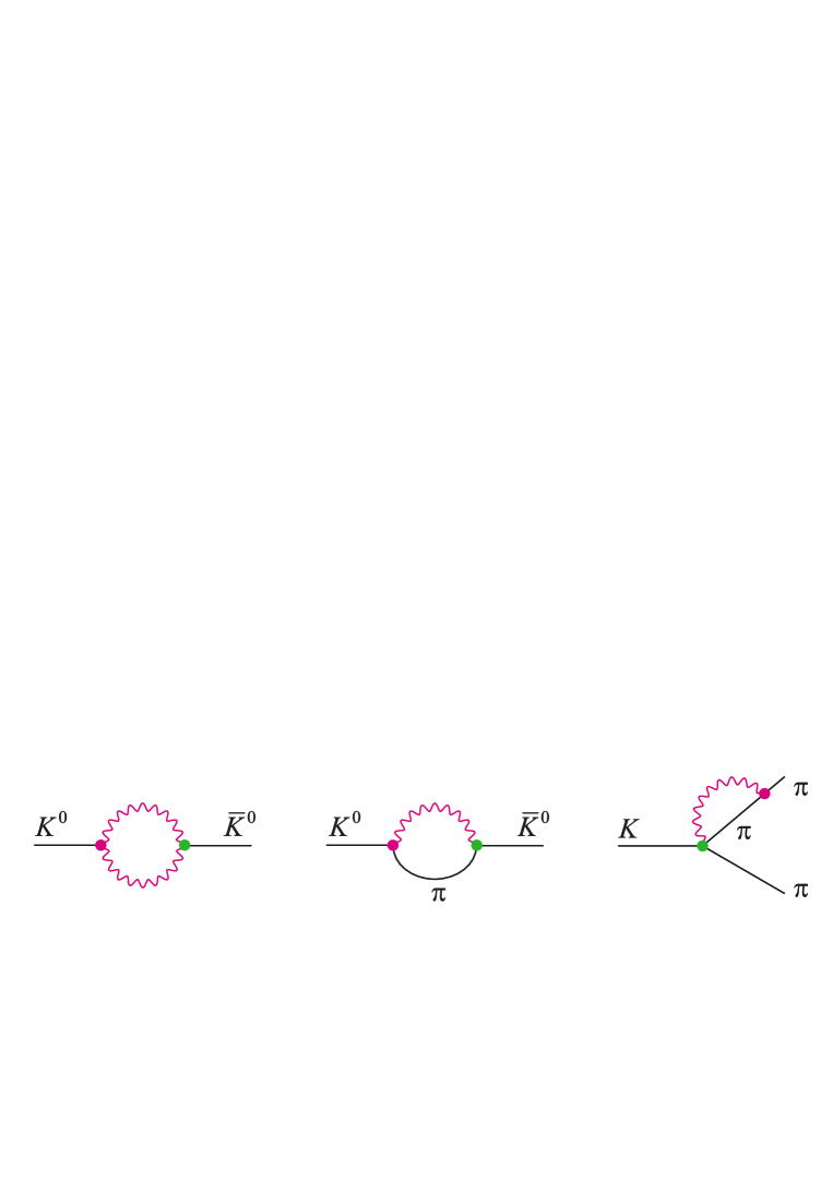
Figure 7: The virtual effects from $Q_{\gamma}^{\pm}$ on $\Delta S=2$ observables (reversed diagrams are understood) and on $\varepsilon^{\prime}$ from $K^{0}\rightarrow\pi^{+}\pi^{-}$. Red vertices stand for the SM transitions (which are not necessarily local, see for example Fig. 5 ), while green vertices are induced by $Q_{\gamma}^{\pm}$.

Let us start with the impact of $Q_{\gamma}^{\pm}$ on $\varepsilon^{\prime}$. The diagram of Fig. 7 induces a correction to $\eta_{+-}=A(K_{L}\rightarrow\pi^{+}\pi^{-})/A(K_{S}\rightarrow\pi^{+}\pi^{-})$ and thereby, discarding strong phases for simplicity

$$\frac{|\operatorname{Re}(\varepsilon^{\prime}/\varepsilon)|_{\gamma}}{\operatorname{Re}(\varepsilon^{\prime}/\varepsilon)^{\exp}}\approx\frac{3\alpha}{256\pi^{3}}B_{T}\frac{G_{F}}{|G_{8}|}\frac{\log(m_{\rho}/m_{\pi})}{|\varepsilon|\operatorname{Re}(\varepsilon^{\prime}/\varepsilon)^{\exp}}\frac{|\operatorname{Im}C_{\gamma}^{-}|}{G_{F}m_{K}}\approx 2\frac{|\operatorname{Im}C_{\gamma}^{-}|}{G_{F}m_{K}}\;.$$ (72)

The photon loop is IR safe since $Q_{\gamma}^{-}$ does not contribute to the bremsstrahlung amplitude in $K^{0}\rightarrow\pi^{+}\pi^{-}\gamma$. Let us stress again that this is only an order of magnitude estimate. Besides the neglected SD mixings, unknown effects of similar size as Eq. (72) are necessarily present to absorb the divergence. Plugging in the bound on $\operatorname{Im}C_{\gamma}^{-}$ obtained from the measured $K^{+}\rightarrow\pi^{+}\pi^{0}\gamma$ direct CP-asymmetry, Eq. (39),

$$(\varepsilon_{+0\gamma}^{\prime})^{\exp}\;\Rightarrow\;\frac{|\operatorname{Re}(\varepsilon^{\prime}/\varepsilon)|_{\gamma}}{\operatorname{Re}(\varepsilon^{\prime}/\varepsilon)^{\exp}}=(16\pm 26)\%\;.$$ (73)

So, even in the presence of a large NP contribution to $Q_{\gamma}^{-}$, the impact on $\varepsilon^{\prime}$ remains smaller than its current theoretical error in the SM.

For completeness, let us also compute the contribution of the magnetic operators to the $\Delta S=2$ observables, for which perturbative QED corrections are significantly suppressed. At long distance, the magnetic operators contribute to $\langle\bar{K}^{0}|H_{W}|K^{0}\rangle$ through the transitions $K^{0}\rightarrow\pi\gamma^{\ast}\rightarrow\bar{K}^{0}$ and $K^{0}\rightarrow\gamma\gamma\rightarrow\bar{K}^{0}$, see Fig. 7. Neglecting the momentum dependences of the $K\rightarrow\gamma\gamma$ and $K\rightarrow\pi\gamma^{\ast}$ vertices and keeping only the leading $\log(m_{\rho}/m_{\pi})$, we obtain

$$\mu_{12}\equiv\frac{\langle\bar{K}^{0}|Q_{\gamma}^{\pm}|K^{0}\rangle}{M_{K}\Delta M_{K}^{\exp}}=(a_{\gamma\gamma}^{\perp}+a_{\pi\gamma})\frac{C_{\gamma}^{+}}{G_{F}m_{K}}+a_{\gamma\gamma}^{||}\frac{C_{\gamma}^{-}}{G_{F}m_{K}}\;,$$ (74)

with (see Eq. (52) for the definition of $A_{\gamma\gamma}^{i}$ and Eq. (136) for that of $a_{S}$)

$$|a_{\gamma\gamma}^{i}| \approx\frac{\alpha^{2}}{72\pi^{3}}B_{T}^{\prime}\frac{G_{F}^{2}m_{K}^{4}F_{\pi}}{\Delta M_{K}^{\exp}}|A_{\gamma\gamma}^{i}|\log(m_{\rho}/m_{K})\approx 7\times 10^{-6}\,|A_{\gamma\gamma}^{i}|\;,$$ (75a)

$$|a_{\pi\gamma}| \approx\frac{\alpha}{512\pi^{5}}B_{T}|a_{S}|\frac{G_{F}^{2}m_{\pi}^{4}m_{K}}{\Delta M_{K}^{\exp}}\log(m_{\rho}/m_{\pi})\approx 8\times 10^{-7}\;.$$ (75b)

Numerically, $a_{\pi\gamma}\sim a_{\pi\gamma}$, even though they are not of the same order in $\alpha$, because of the absence of a $K^{0}\rightarrow\pi^{0}\gamma^{\ast}$ vertex at leading order (see Eq. (136) in Appendix B), and because the momentum scale in the $a_{\pi\gamma}$ loop is entirely set by the pion mass instead of the transferred momentum of $\mathcal{O}(m_{K})$, as in $a_{\gamma\gamma}$. With such small values for $a_{\gamma\gamma}$ and $a_{\pi\gamma}$, neither $\Delta M_{K}(Q_{\gamma}^{\pm})\sim\operatorname{Re}\mu_{12}$ nor $\varepsilon_{K}(Q_{\gamma})\sim\operatorname{Im}\mu_{12}$ can compete with the non-radiative $\Delta S=2$ processes, even in the presence of NP in $Q_{\gamma}^{\pm}$.

3.4.2 Gluonic penguin operators

In complete analogy with the electromagnetic operators, gluonic FCNC are described by effective operators of dimensions greater than four. For instance, the chromomagnetic operators producing either a real or a virtual gluon are

$$\mathcal{H}_{eff}^{\gamma}=C_{g}^{\pm}Q_{g}^{\pm}+h.c.\;,\;\;\;Q_{g}^{\pm}=\frac{g}{16\pi^{2}}(\bar{s}_{L}\sigma^{\alpha\beta}t^{a}d_{R}\pm\bar{s}_{R}\sigma^{\alpha\beta}t^{a}d_{L})G_{\alpha\beta}^{a}\;.$$ (76)

The chromoelectric operators $Q_{g^{\ast}}^{\pm}$, whose form can easily be deduced from Eq. (2), contribute only for a virtual gluon.

In the SM, both $Q_{g}^{\pm}$ and $Q_{g^{\ast}}^{\pm}$ arise from the diagram shown in Fig. 8. As for $Q_{\gamma}^{\pm}$, the former are suppressed by the light-quark chirality flips hence completely negligible, but the chromoelectric operators are sizeable and enter into the initial conditions for the four-quark operators [6]. They are thus hidden inside the weak low-energy constants in Eq. (15), together with the hadronic virtual photon and $Z$ penguins (see Fig. 2).

Figure 8: The gluonic penguin in the SM.

The chromomagnetic operators are not included in the standard OPE, since they are negligible in the SM. But being of dimension-five, they could get significantly enhanced by NP. This would have two main effects. First, through the OPE mixing, $Q_{g}^{\pm}$ generate $Q_{\gamma}^{\pm}$. When both arise at a high-scale $\mu_{NP}\gtrsim M_{W}$, assuming only the SM colored particle content, neglecting the mixings with the four-quark operators, and working to LO [65]:

$$C_{\gamma}^{\pm}(\mu_{c}) =\eta^{2}\left[C_{\gamma}^{\pm}(\mu_{NP})+8(1-\eta^{-1})C_{g}^{\pm}(\mu_{NP})\right]\;,\;\;C_{g}^{\pm}(\mu_{c})=\eta C_{g}^{\pm}(\mu_{NP})\;,$$

$$\eta \equiv\eta(\mu_{NP})=\left(\frac{\alpha_{S}(\mu_{NP})}{\alpha_{S}(m_{t})}\right)^{2/21}\left(\frac{\alpha_{S}(m_{t})}{\alpha_{S}(m_{b})}\right)^{2/23}\left(\frac{\alpha_{S}(m_{b})}{\alpha_{S}(\mu_{c})}\right)^{2/25}\;.$$ (77)

Numerically, $\eta(\mu)=0.90,0.89,0.88$ for $\mu=0.1,0.5,1$ TeV, respectively. Indirectly, all the bounds on $C_{\gamma}^{\pm}$ can thus be translated as bounds on $C_{g}^{\pm}$.

However, there is another more direct impact of $Q_{g}^{\pm}$ on phenomenology since it contributes to $K\rightarrow\pi\pi$, hence to $\varepsilon^{\prime}$ [65]

$$\operatorname{Re}(\varepsilon^{\prime}/\varepsilon)_{g}=\frac{11}{64\pi^{2}}\frac{\omega}{|\varepsilon||\operatorname{Re}A_{0}|}\frac{m_{\pi}^{2}m_{K}^{2}}{F_{\pi}(m_{s}+m_{d})}\eta B_{G}\operatorname{Im}C_{g}^{-}\approx 3B_{G}\frac{\operatorname{Im}C_{g}^{-}}{G_{F}m_{K}}\;,$$ (78)

with, neglecting $\Delta I=3/2$ contributions, $|\operatorname{Re}A_{0}|=\sqrt{2}F_{\pi}(m_{K}^{2}-m_{\pi}^{2})|\operatorname{Re}G_{8}|$ and $F_{\pi}=92.4$ MeV. The hadronic parameter $B_{G}$ parametrizes the departure of $\langle(\pi\pi)_{0}|Q_{g}^{-}|K^{0}\rangle$ from the chiral quark model, and lies presumably in the range $1\rightarrow 4$ [65]. Given that the SM prediction for $\operatorname{Re}(\varepsilon^{\prime}/\varepsilon)$ is rather close to $\operatorname{Re}(\varepsilon^{\prime}/\varepsilon)^{\exp}$ [50], but its uncertainty is itself of the order of $\operatorname{Re}(\varepsilon^{\prime}/\varepsilon)^{\exp}$, we simply impose that $|\operatorname{Re}(\varepsilon^{\prime}/\varepsilon)_{g}|\leq\operatorname{Re}(\varepsilon^{\prime}/\varepsilon)^{\exp}$, which gives,

$$\frac{|\operatorname{Im}C_{g}^{-}|}{G_{F}m_{K}}\lesssim 5\times 10^{-4}\;.$$ (79)

For comparison, imposing that $\left|\operatorname{Re}A_{0}\right|_{g}$ is at most of the order of $\left|\operatorname{Re}A_{0}\right|^{\exp}$ gives the much looser constraint $|\operatorname{Re}C_{g}^{-}|/G_{F}m_{K}\lesssim 10$. Note, however, that the bound (79) is not to be taken too strictly. First, the $B_{G}$ parameter is set to $1$, but could be slightly smaller or bigger. Second, $Q_{g}^{\pm}$ is not the only FCNC affecting $\operatorname{Re}(\varepsilon^{\prime}/\varepsilon)$ (see Fig. 2). This bound could get relaxed in the presence of NP in the other penguins. This will be analyzed in more details in the next section.

4 New Physics effects

In most models of New Physics, new degrees of freedom and additional sources of flavor breaking offer alternative mechanisms to induce the FCNC transitions. The goal of the present section is to quantify the possible phenomenological impacts of NP in the dimension-five magnetic operators $Q_{\gamma}^{\pm}$ of Eq. (1). As discussed in details in the previous sections, CP-conserving processes are fully dominated by the SM long-distance contributions. So, throughout this section, we concentrate exclusively on CP-violating observables, from which the short-distance physics can be more readily accessed along with possible signals of NP.

The cleanest observables to identify a large enhancement of $Q_{\gamma}^{\pm}$ are the direct CP-asymmetries in $K\rightarrow\pi\pi\gamma$ and $K\rightarrow(\gamma\gamma)_{||}$, which would then satisfy

$$\frac{1}{3}|\varepsilon_{+0\gamma}^{\prime}(Q_{\gamma}^{-})|\approx 5|\varepsilon_{+-\gamma}^{\prime}(Q_{\gamma}^{-})|\approx 3|\varepsilon_{||}^{\prime}(Q_{\gamma}^{-})|\approx\frac{|\operatorname{Im}C_{\gamma}^{-}|}{G_{F}m_{K}}\;.$$ (80)

Indeed, the contributions from the four-quark operators (QCD and electroweak penguins) is small and under control,

$$\frac{3\omega}{2\sqrt{2}}|\varepsilon_{+0\gamma}^{\prime}(Q_{3,...,10})|\approx\frac{5}{2}|\varepsilon_{+-\gamma}^{\prime}(Q_{3,...,10})|\approx|\varepsilon_{||}^{\prime}(Q_{3,...,10})|\approx|\varepsilon^{\prime}|\;,$$ (81)

with $\omega=1/22.4$. By using the experimental $\varepsilon^{\prime}$ value, these estimates are independent of the presence of NP in $Q_{3,...,10}$. On the other hand, the $K_{S,L}\rightarrow(\gamma\gamma)_{\perp}$ asymmetry is very sensitive to $\Omega$, representing the ratio of the electroweak to the QCD penguin contributions in $\varepsilon^{\prime}$:

$$\varepsilon_{\perp}^{\prime}(Q_{3,...,10})=-i\frac{\operatorname{Im}A_{0}}{\operatorname{Re}A_{0}}=i\frac{\sqrt{2}|\varepsilon^{\prime}|}{\omega(1-\Omega)}\;\;,\;\;\;\;|\varepsilon_{\perp}^{\prime}(Q_{\gamma}^{+})|\approx\frac{1}{2}\frac{|\operatorname{Im}C_{\gamma}^{+}|}{G_{F}m_{K}}\;.$$ (82)

So, knowing the impact of $Q_{\gamma}^{+}$, the asymmetry $\varepsilon_{\perp}^{\prime}$ can be used to extract the otherwise inaccessible QCD penguin contributions to $\varepsilon^{\prime}$.

The experimental information on these four asymmetries is however limited, with only the loose bound (31) on $\varepsilon_{+0\gamma}^{\prime}$ and (44) on $\varepsilon_{+-\gamma}^{\prime}$ currently available. So, to get some information on $Q_{\gamma}^{\pm}$, two routes will be explored.

First, we can use the $K_{L}\rightarrow\pi^{0}\ell^{+}\ell^{-}$ decay rates, for which the experimental bounds are currently in the $10^{-10}$ range. As shown in Fig. 9, these modes are rather sensitive to $Q_{\gamma}^{+}$ once $|\operatorname{Im}C_{\gamma}^{+}|/G_{F}m_{K}$ is above a few $10^{-3}$. In the absence of any other source of NP, the experimental bounds (67) give

$$K_{L}\overset{}{\rightarrow}\pi^{0}e^{+}e^{-} \Rightarrow\;-0.018<\frac{\operatorname{Im}C_{\gamma}^{+}}{G_{F}m_{K}}<+0.030\;,$$ (83a)

$$K_{L}\overset{}{\rightarrow}\pi^{0}\mu^{+}\mu^{-} \Rightarrow\;-0.050<\frac{\operatorname{Im}C_{\gamma}^{+}}{G_{F}m_{K}}<+0.063\;.$$ (83b)

To compare with the direct CP-asymmetries (80), sensitive to $Q_{\gamma}^{-}$, we first need to study how NP could affect the relationship between $Q_{\gamma}^{+}$ and $Q_{\gamma}^{-}$. If the SM relation $C_{\gamma}^{+}\approx-C_{\gamma}^{-}$ survives, the direct CP-asymmetries could be relatively large, with for example $-8\%<\varepsilon_{+0\gamma}^{\prime}<5\%$ from $K_{L}\rightarrow\pi^{0}e^{+}e^{-}$. Then, since NP can enter in $K_{L}\rightarrow\pi^{0}\ell^{+}\ell^{-}$ through other FCNC, for example by affecting the electroweak penguins, we must also study their possible interferences with $Q_{\gamma}^{+}$, and quantify how broadly the bounds (83) could get relaxed.

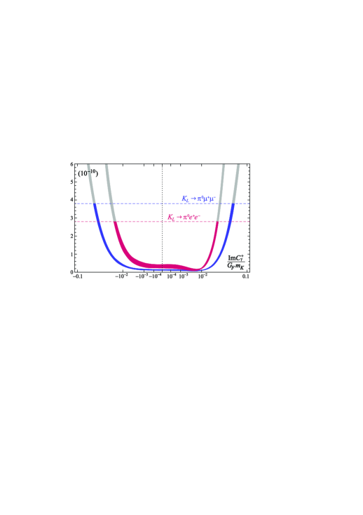
Figure 9: The sensitivity of the $K_{L}\rightarrow\pi^{0}\ell^{+}\ell^{-}$ decays to the magnetic penguin operator $Q_{\gamma}^{+}$, in the absence of any other source of NP. These curves are actually parabolas, but blown out to emphasize the small $\operatorname{Im}C_{\gamma}^{+}/G_{F}m_{K}$ region (whose SM value is in the $10^{-5}$ range). The horizontal lines signal the experimental bounds on $K_{L}\rightarrow\pi^{0}\ell^{+}\ell^{-}$. The contours stand for $90\%$ confidence regions given the current theoretical errors in Eq. (63). Their apparent thinning as $|\operatorname{Im}C_{\gamma}^{+}|$ increases is purely optical, except just below $10^{-2}$ where the $Q_{\gamma}^{+}$ contribution precisely cancel out with the SM one in the vector current (positive DCPV–ICPV interference is assumed).

A second route is to use $\varepsilon^{\prime}$. Indeed, in many NP models, the magnetic operators $Q_{\gamma}^{\pm}$ are accompanied by chromomagnetic operators $Q_{g}^{\pm}$, which contribute directly to $\varepsilon^{\prime}$,

$$\operatorname{Re}(\varepsilon^{\prime}/\varepsilon)_{g}\approx 3B_{G}\frac{\operatorname{Im}C_{g}^{-}}{G_{F}m_{K}}\;,$$ (84)

with $B_{G}$ the hadronic bag parameter a priori of $\mathcal{O}(1)$. If the Wilson coefficients of $Q_{\gamma}^{\pm}$ and $Q_{g}^{\pm}$ are similar, the current measurement $\operatorname{Re}(\varepsilon^{\prime}/\varepsilon)^{\exp}=(1.65\pm 26)\times 10^{-3}$ [18] imposes strong constraints, and would naively imply that the direct CP-asymmetries in Eq. (80) are at most of $\mathcal{O}(10^{-3})$. However, not only the relationship between $Q_{g}^{\pm}$ and $Q_{\gamma}^{\pm}$ is model-dependent, but as for $K_{L}\rightarrow\pi^{0}\ell^{+}\ell^{-}$, many other FCNC enter in $\varepsilon^{\prime}$ and their possible correlations with $Q_{g}^{\pm}$ must be analyzed.

The only way to relate the NP occurring in the various FCNC is to adopt a specific picture for the NP dynamics. Evidently, this cannot be done model-independently. Instead, the strategy will be to classify the models into broad classes, and within each class, to stay as model-independent as possible. In practice, these classes are in one-to-one correspondence with the choice of basis made for the effective semileptonic FCNC operators. Once a basis is chosen, bounds on the Wilson coefficients of these operators are derived by turning them on one at a time. In this way, fine-tunings between the chosen operators are explicitly ruled out. This is where the model-dependence enters [67]. On the other hand, the magnetic operators are kept on at all times, since it is precisely their interference with the semileptonic FCNC which we want to resolve. Note that the alternative procedure of performing a full scan over parameter space is (usually) basis independent, but we prefer to avoid that method as the many possible fine-tuning among the semileptonic operators would obscure those with the magnetic ones. Further, we will see that with our method, it is possible to get additional insight because the bounds do depend on the basis, and thus allow discriminating among the NP scenarios.

4.1 Model-independent analysis

The most model-independent operator basis is the one minimizing the interferences between the NP contributions in physical observables [67]. It is the one in Eq. (61), which we reproduce here for convenience:

$$\mathcal{H}_{\text{Pheno}}=-\frac{G_{F}\alpha}{\sqrt{2}}\sum_{\ell=e,\mu,\tau}(C_{\nu,\ell}\;Q_{\nu,\ell}+C_{V,\ell}\;Q_{V,\ell}+C_{A,\ell}\;Q_{A,\ell})+C_{\gamma}^{\pm}Q_{\gamma}^{\pm}+h.c.\;,$$ (85)

$$Q_{V,\ell}=\bar{s}\gamma^{\mu}d\otimes\bar{\ell}\gamma_{\mu}\ell\;,\;\;Q_{A,\ell}=\bar{s}\gamma^{\mu}d\otimes\bar{\ell}\gamma_{\mu}\gamma_{5}\ell\;,\;\;Q_{\nu,\ell}=\bar{s}\gamma^{\mu}d\otimes\bar{\nu}_{\ell}\gamma_{\mu}(1-\gamma_{5})\nu_{\ell}\;,$$

$$Q_{\gamma}^{\pm}=\frac{Q_{d}e}{16\pi^{2}}\;(\bar{s}_{L}\sigma^{\mu\nu}d_{R}\pm\bar{s}_{R}\sigma^{\mu\nu}d_{L})\,F_{\mu\nu}\;.$$

The four-fermion operators do not interfere in the rates since they produce different final states, while $Q_{\gamma}^{+}$ and $Q_{\gamma}^{-}$ have opposite CP-properties (see Table 1). On the other hand, $Q_{\gamma}^{\pm}$ and $Q_{V,\ell}\ni Q_{\gamma^{\ast}}^{\pm}$ involve an intermediate photon hence necessarily interfere. Note that the coefficients in Eq. (85) are understood to be purely induced by the NP: the SM contributions have to be added separately.

Given the current data, the bounds on the CP-violating parts of the Wilson coefficients are (we define $\rho^{-1}\equiv 21.3G_{F}m_{K}$ from Eq. (70))

$$\begin{array}[c]{rc}K^{+}\rightarrow\pi^{+}\pi^{0}\gamma\Rightarrow&-160<\rho\operatorname{Im}C_{\gamma}^{-}<80\;,\vskip 3.0pt plus 1.0pt minus 1.0pt\\ K_{L}\rightarrow\pi^{0}e^{+}e^{-}\Rightarrow&-14<\operatorname{Im}C_{V,e}-\rho\operatorname{Im}C_{\gamma}^{+}<\;\;8\oplus[-10<\operatorname{Im}C_{A,e}<11\wedge\;\;-8<\rho\operatorname{Im}C_{\gamma}^{+}<14]\;,\vskip 3.0pt plus 1.0pt minus 1.0pt\\ K_{L}\rightarrow\pi^{0}\mu^{+}\mu^{-}\Rightarrow&-29<\operatorname{Im}C_{V,\mu}-\rho\operatorname{Im}C_{\gamma}^{+}<24\oplus[-16<\operatorname{Im}C_{A,\mu}<18\wedge-24<\rho\operatorname{Im}C_{\gamma}^{+}<29]\;,\vskip 3.0pt plus 1.0pt minus 1.0pt\\ K^{+}\rightarrow\pi^{+}\nu\bar{\nu}\;\Rightarrow&-14<\operatorname{Im}C_{\nu,\ell}<17\;\;(\ell=e\oplus\mu\oplus\tau)\;.\end{array}$$ (86)

All the numbers are in unit of $10^{-4}$. The symbol “$\oplus$” stands for the exclusive alternative, since e.g. $C_{A,\ell}$ and $C_{V,\ell}$ are not turned on simultaneously, while “$\Lambda$” means that the bounds are correlated, i.e. the coefficients fall within an elliptical contour in the corresponding plane. For comparison, $\operatorname{Im}C_{V,\ell}^{\text{SM}}$, $\operatorname{Im}C_{A,\ell}^{\text{SM}}$ and $\operatorname{Im}C_{\nu,\ell}^{\text{SM}}$ are all around $10^{-4}$. For the magnetic operators, the SM value in Eq. (12) implies $\rho\operatorname{Im}C_{\gamma}^{\pm,\text{SM}}\approx\mp 0.015\operatorname{Im}\lambda_{t}\sim\mathcal{O}(10^{-6})$.

For the neutrino modes, NP is separately turned on in each $\operatorname{Im}C_{\nu,\ell}$, $\ell=e,\mu,\tau$. Assuming leptonic universality would decrease the bound by about $\sqrt{3}$ since then all three $C_{\nu,e}=C_{\nu,\mu}=C_{\nu,\tau}$ would simultaneously contribute. The direct bounds on $\operatorname{Im}C_{\nu,\ell}$ from $K_{L}\rightarrow\pi^{0}\nu\bar{\nu}$ are currently not competitive, so the experimental bound on the $K^{+}\rightarrow\pi^{+}\nu\bar{\nu}$ mode is used setting $\operatorname{Re}C_{\nu,\ell}=0$. The maximal value for $K_{L}\rightarrow\pi^{0}\nu\bar{\nu}$ can then be predicted

$$\mathcal{B}(K_{L}\rightarrow\pi^{0}\nu\bar{\nu})<1.2\times 10^{-9}\;,$$ (87)

which corresponds to a saturation of the Grossman-Nir Bound [68] (including the isospin breaking effects in the vector form-factor, but forbidding a destructive interference between the CP-conserving SM and NP contributions since $\operatorname{Re}C_{\nu,\ell}=0$). This is more than an order of magnitude below the current experimental limit, but about 50 times larger than the SM prediction.

For $K_{L}\rightarrow\pi^{0}\ell^{+}\ell^{-}$, the bound on the vector current is less strict than on the axial-vector current because of the interference with the indirect CP-violating contribution. The theoretically favored case of positive DCPV-ICPV interference is assumed (relaxing this would not change much the numbers). Finally, the impact of $Q_{\gamma}^{-}$ on $\varepsilon^{\prime}$ is estimated to be below $30\%$ of its experimental value given the bound from $K^{+}\rightarrow\pi^{+}\pi^{0}\gamma$, see Eq. (73), hence is neglected.

Figure 10: The band in the $\operatorname{Im}C_{V,\ell}-\operatorname{Im}C_{\gamma}^{+}$ plane allowed by the $K_{L}\rightarrow\pi^{0}\ell^{+}\ell^{-}$ experimental bounds. The degree of fine-tuning is represented by the lighter areas, where $|\operatorname{Im}C_{V,\ell}-\rho\operatorname{Im}C_{\gamma}^{+}|/|\rho\operatorname{Im}C_{\gamma}^{+}|<1/r$, $r=2,5,10,30$. Assuming $\operatorname{Im}C_{\gamma}^{+}=-\operatorname{Im}C_{\gamma}^{-}$, $\varepsilon_{+0\gamma}^{\prime}$ could thus reach its $K^{+}\rightarrow\pi^{+}\pi^{0}\gamma$ experimental bound for $r\gtrsim 5$.

To resolve the bound in the vector current and thereby disentangle $C_{\gamma}^{+}$ and $C_{V,\ell}$, one is forced to specify at which level a destructive interference becomes a fine-tuning, see Fig. 10. This introduces some model-dependence since a specific NP model could generate $Q_{\gamma}^{\pm}$ and $Q_{V,\ell}$ (or $Q_{\gamma^{\ast}}^{\pm}$) coherently. In this respect, it should be noted that the basis of four-fermion operators in Eq. (85) is not complete. It lacks the scalar, pseudoscalar, tensor and pseudotensor four-fermion operators. Naively, all these operators produce the lepton pair in different states and do not interfere in the rate [34]. Introducing large NP in any of them would thus render the bounds (86) weaker. There is however one exception. In $K_{L}\rightarrow\pi^{0}\ell^{+}\ell^{-}$, the tensor operators,

$$Q_{T,\ell}=\bar{s}\sigma^{\mu\nu}d\otimes\bar{\ell}\sigma_{\mu\nu}\ell\;,$$ (88)

do produce the leptons in the same $1^{--}$ state as $Q_{V,\ell}$ and $Q_{\gamma}^{+}$ [34]. So, effectively, $Q_{T,\ell}$ can be absorbed into $Q_{V,\ell}$. But then, owing to their similar structures, it is not impossible that $Q_{\gamma}^{\pm}$ and $Q_{T,\ell}$ are generated simultaneously, and thus that $Q_{\gamma}^{\pm}$ is tightly correlated to this effective $Q_{V,\ell}$.

In the next two sections, several NP scenarios are considered, in order to investigate under which circumstances the bounds on $C_{\gamma}^{+}$ and $C_{V,\ell}$ can be resolved. Of course, ultimately, better measurements of the direct CP-asymmetries are the cleanest option to get to $C_{\gamma}^{\pm}$. But before pushing for an experimental effort in that direction, it is essential to have a more precise idea of their maximal sizes under a large spectrum of NP scenarios.

4.1.1 Hadronic current and Minimal Flavor Violation

The NP scenarios are organized into two broad classes according to the way the leptonic currents of the effective operators are parametrized. So, before entering that discussion, let us consider here their hadronic parts, whose generic features transcend the various scenarios.

Only the vector current $\bar{s}\gamma_{\mu}d$ enters in Eq. (85) because the axial-vector current $\bar{s}\gamma_{\mu}\gamma_{5}d$ drops out of the $K\rightarrow\pi\nu\bar{\nu}$ and $K_{L}\rightarrow\pi^{0}\ell^{+}\ell^{-}$ matrix elements. It would thus be equivalent to replace $\bar{s}\gamma_{\mu}d$ by the $SU(2)_{L}\otimes U(1)_{Y}$ invariant forms $\bar{Q}\gamma_{\mu}Q$ and $\bar{D}\gamma_{\mu}D$, with $Q^{T}=(u,d)_{L}$ and $D=d_{R}$. By contrast, the magnetic operators require an extra Higgs doublet field to reach an $SU(2)_{L}$ invariant form:

$$Q_{\gamma}^{\pm}\sim(\bar{Q}\sigma^{\mu\nu}DH\pm\bar{D}\sigma^{\mu\nu}QH^{\ast})\,F_{\mu\nu}\;.$$ (89)

After electroweak symmetry breaking, this operator collapses to that in Eq. (2). Consequently, if the NP respects the $SU(2)_{L}\otimes U(1)_{Y}$ symmetry, $Q_{\gamma}^{\pm}$ and semileptonic operators are equally suppressed by the NP scale since they are all of dimension six. However, the magnetic operators are a priori much more sensitive to the electroweak symmetry breaking mechanism, so that the scaling between the two types of operators cannot be assessed model-independently. Its phenomenological extraction is thus important, and could help discriminate among models.

The effective operators in Eq. (85) induce the $s\rightarrow d$ flavor transition, while the leptonic currents (or the photon) are flavor diagonal. Model-independently, the underlying gauge symmetry properties of an operator does not preclude anything about its flavor-breaking capabilities. However, the situation changes if we ask for the NP to have no more sources of flavor breaking than the SM. This is the Minimal Flavor Violation hypothesis [69]. For the operators at hand, it implies that the hadronic currents scale as

$$\bar{Q}^{I}\gamma_{\mu}(\mathbf{Y}_{u}^{\dagger}\mathbf{Y}_{u})^{IJ}Q^{J}\;,\;\;\bar{D}^{I}\gamma_{\mu}(\mathbf{Y}_{d}\mathbf{Y}_{u}^{\dagger}\mathbf{Y}_{u}\mathbf{Y}_{d}^{\dagger})^{IJ}D^{J}\;,\;\;\bar{Q}^{I}\sigma^{\mu\nu}(\mathbf{Y}_{u}^{\dagger}\mathbf{Y}_{u}\mathbf{Y}_{d})^{IJ}D^{J}\;,$$ (90)

with $v\mathbf{Y}_{d}=\mathbf{m}_{d}$, $v\mathbf{Y}_{u}=\mathbf{m}_{u}V$, $\mathbf{m}_{u,d}$ the diagonal quark mass matrices, and $v$ the Higgs vacuum expectation value. The CKM matrix $V$ is put in $\mathbf{Y}_{u}$ so that the down-quark fields in the operators of Eq. (85) are mass eigenstates. Also, we limit the MFV expansions to the leading sources of flavor-breaking (i.e., minimal number of $\mathbf{Y}_{u,d}$) for simplicity.

Under MFV, the NP operators acquire many SM-like properties. First, $\bar{D}\gamma_{\mu}D$ is doubly suppressed by the light quark Yukawa couplings, and is thus not competitive with $\bar{Q}\gamma_{\mu}Q$. Second, the chirality flip in $\bar{Q}^{I}\sigma^{\mu\nu}D^{J}$ comes from the external light quark masses, and are thus significantly suppressed. Finally, the $s\rightarrow d$ transitions become correlated to the $b\rightarrow d$ and $b\rightarrow s$ transitions since

$$v^{2}(\mathbf{Y}_{u}^{\dagger}\mathbf{Y}_{u})^{IJ}\approx m_{t}^{2}V_{3I}^{\dagger}V_{3J}^{\,}\;.$$ (91)

Of course, this correlation is not always strict as additional terms in the MFV expansion can be relevant. Still, it drives the overall scale of the observables in each sector.

We do not intend to perform a full MFV analysis here. Instead, our goal is to quantify, under the MFV ansatz, the maximal NP effects $Q_{\gamma}^{\pm}$ could induce given the current situation in $b\rightarrow s\gamma$. From Eqs. (89, 90, 91), discarding $m_{s(d)}$ against $m_{b(s)}$,

$$Q_{\gamma}^{\pm}|_{d_{R}^{I}\rightarrow d_{L}^{J}}\sim C_{7\gamma}(\mu_{EW})\;(\bar{Q}^{J}\sigma^{\mu\nu}(\mathbf{Y}_{u}^{\dagger}\mathbf{Y}_{u}\mathbf{Y}_{d})^{JI}D^{I})\;H\;F_{\mu\nu}\;\;\;\Rightarrow\frac{Q_{\gamma}^{\pm}|_{s\rightarrow d}}{Q_{\gamma}^{\pm}|_{b\rightarrow s}}\sim\frac{V_{ts}^{\dagger}V_{td}\;m_{s}}{V_{ts}^{\dagger}V_{tb}\;m_{b}}\;.$$ (92)

The flavor-universality of the Wilson coefficient $C_{7\gamma}(\mu_{EW})$ embodies the MFV hypothesis. The NP shift still allowed by $b\rightarrow s\gamma$ is [70]

$$\delta C_{7\gamma}(\mu_{EW})=[-0.14,0.06]\cup[1.42,1.62]\;,$$ (93)

for constructive and destructive interference with the SM contributions. The latter has a lower probability, and would require significant cancellations among the NP effects in $B\rightarrow X_{s}\ell^{+}\ell^{-}$. From Eq. (12), and including the LO QCD reduction [6], such a shift can be written in our conventions as

$$\frac{\left.\operatorname{Im}C_{\gamma}^{\pm}\right|_{\text{MFV}}}{G_{F}m_{K}}-\frac{\left.\operatorname{Im}C_{\gamma}^{\pm}\right|_{\text{SM}}}{G_{F}m_{K}}\approx\pm\frac{2}{3}\,\operatorname{Im}\lambda_{t}\,\delta C_{7\gamma}(\mu_{EW})\;.$$ (94)

For comparison, the SM prediction is $\mp 0.31(8)\times\operatorname{Im}\lambda_{t}$. So, there would be no visible effects for $\delta C_{7\gamma}(\mu_{EW})\in[-0.14,0.06]$, and at most a factor four enhancement for $\delta C_{7\gamma}(\mu_{EW})\in[1.42,1.62]$.

This is hardly sufficient to push any of the asymmetries within the experimentally accessible range, while the impact on $K_{L}\rightarrow\pi^{0}\ell^{+}\ell^{-}$ would be buried in the theoretical errors, see Fig. 9. However, it is well-known that MFV is particularly effective for $K$ physics since it suppresses the NP contributions by the small $V_{ts}^{\ast}V_{td}\sim 10^{-4}$. So, this is the best place to test MFV. A deviation with respect to the strict ansatz (92) could lead to visible effects.

4.2 Tree-level FCNC

The basis of operators in Eq. (85) maximally breaks the $SU(2)_{L}\otimes U(1)_{Y}$ symmetry. Neutrinos are completely decoupled from the charged leptons, and the vector and axial-vector operators (as well as $Q_{\gamma}^{+}$ and $Q_{\gamma}^{-}$) maximally mix currents of opposite chiralities. To be specific, the $SU(2)_{L}\otimes U(1)_{Y}$ invariant basis [71] is, after projecting the hadronic currents of semileptonic operators on their vector components,

$$\mathcal{H}_{\text{Gauge}}=-\frac{G_{F}\alpha}{\sqrt{2}}\sum_{\ell=e,\mu,\tau}(C_{L,\ell}\;Q_{L,\ell}+C_{L,\ell}^{\prime}\;Q_{L,\ell}^{\prime}+C_{R,\ell}\;Q_{R,\ell})+C_{\gamma}^{L,R}Q_{\gamma}^{L.R}+h.c.\;,$$ (95)

$$Q_{L}\equiv\bar{s}\gamma^{\mu}d\otimes\bar{L}\gamma_{\mu}L\;,\;\;Q_{L}^{\prime}\equiv\bar{s}\gamma^{\mu}d\otimes\bar{L}\gamma_{\mu}\sigma^{3}L\;,\;\;Q_{R}\equiv\bar{s}\gamma^{\mu}d\otimes\bar{E}\gamma_{\mu}E\;\;,$$

$$Q_{\gamma}^{L}=\frac{Q_{d}e}{16\pi^{2}v}\;\bar{s}_{R}\sigma^{\mu\nu}d_{L}\,H^{\ast}\,F_{\mu\nu}\;,\;\;\,Q_{\gamma}^{R}=\frac{Q_{d}e}{16\pi^{2}v}\;\bar{s}_{L}\sigma^{\mu\nu}d_{R}\,H\,F_{\mu\nu}\;,$$

with $L^{T}=(\nu_{\ell},\ell)_{L}$ and $E=\ell_{R}$. It is related to the phenomenological basis (85) through nearly democratic transformations

$$\left(\begin{array}[c]{c}C_{\nu,\ell}\\ C_{V,\ell}\\ C_{A,\ell}\end{array}\right)=\frac{1}{2}\left(\begin{array}[c]{ccc}1&1&0\\ 1&-1&1\\ -1&1&1\end{array}\right)\left(\begin{array}[c]{c}C_{L,\ell}\\ C_{L,\ell}^{\prime}\\ C_{R,\ell}\end{array}\right)\;,\;\left(\begin{array}[c]{c}C_{\gamma}^{-}\\ C_{\gamma}^{+}\end{array}\right)=\frac{1}{2}\left(\begin{array}[c]{cc}1&-1\\ 1&1\end{array}\right)\left(\begin{array}[c]{c}C_{\gamma}^{R}\\ C_{\gamma}^{L}\end{array}\right)\;,$$ (96)

for each $\ell=e,\mu,\tau$. As in Eq. (85), the SM contributions are not encoded into $\mathcal{H}_{\text{Gauge}}$, and have to be added separately.

The $\mathcal{H}_{\text{Gauge}}$ basis represents a class of models where the four-fermion effective operators arise entirely from some high-scale $SU(2)_{L}\otimes U(1)_{Y}$ invariant tree-level interactions. It is characterized by the correlations it imposes among the phenomenologically non interfering operators in $\mathcal{H}_{\text{Pheno}}$. A well-known example of model within this class is the MSSM with R-parity violating couplings [72], but more generic leptoquark models are also of this form [73]. Note that in these two cases, the $Q_{\gamma}^{R,L}$ operators nevertheless arise only at the loop level since both the photon and the Higgs (see Eq. (89)) have flavor-diagonal couplings at tree-level.

The $\mathcal{H}_{\text{Gauge}}$ basis completely decouples the three leptonic flavors. This is adequate since generic leptoquark couplings do not respect leptonic universality. Actually, one would expect that lepton-flavor violating (LFV) operators should arise, inducing in particular $K\rightarrow(\pi)e\mu$ which corresponds to an $s+\mu\rightarrow d+e$ transition. Those modes are very constrained experimentally, with bounds often lower that for lepton-flavor conserving (LFC) modes. So, if LFV and LFC couplings have similar sizes, there can be no large effects in the LFC modes. However, to relate the LFC and LFV couplings is far from immediate, and requires some additional inputs on the dynamics (see e.g. Ref.[74] for studies within MFV). So in the present work, we concentrate exclusively on LFC decay channels. Still, let us emphasize again that leptonic universality is not expected to hold in the present scenario.

Adopting the $SU(2)_{L}\otimes U(1)_{Y}$ invariant basis, the Wilson coefficients of the semileptonic operators in Eq. (95) are turned on one at a time while either $C_{\gamma}^{L}$ or $C_{\gamma}^{R}$ is kept on. The bounds are then completely resolved and rather strict (all numbers in units of $10^{-4}$)

$$\begin{array}[c]{rc}K_{L}\rightarrow\pi^{0}e^{+}e^{-}\Rightarrow&-20<(-\operatorname{Im}C_{L,e}\oplus\operatorname{Im}C_{L,e}^{\prime}\oplus\operatorname{Im}C_{R,e})<24\;\;\wedge\;\;-14<\rho\operatorname{Im}C_{\gamma}^{+}<19\;,\vskip 3.0pt plus 1.0pt minus 1.0pt\\ K_{L}\rightarrow\pi^{0}\mu^{+}\mu^{-}\Rightarrow&-33<(-\operatorname{Im}C_{L,\mu}\oplus\operatorname{Im}C_{L,\mu}^{\prime}\oplus\operatorname{Im}C_{R,\mu})<37\;\;\wedge\;\;-30<\rho\operatorname{Im}C_{\gamma}^{+}<36\;,\vskip 3.0pt plus 1.0pt minus 1.0pt\\ K^{+}\rightarrow\pi^{+}\nu\bar{\nu}\;\Rightarrow&-28<(\operatorname{Im}C_{L,\ell}\oplus\operatorname{Im}C_{L,\ell}^{\prime})<34\;\;(\ell=e\oplus\mu\oplus\tau)\;.\end{array}$$ (97)

Indeed, $C_{\gamma}^{L}$ and $C_{\gamma}^{R}$ cannot grow unchecked since the bounds from $K_{L}\rightarrow\pi^{0}(\ell^{+}\ell^{-})_{1^{--}}$ would then require a large interference with $C_{L}$, $C_{L}^{\prime}$, or $C_{R}$ . But these Wilson coefficients also contribute either to the neutrino modes (via $Q_{\nu,\ell}$) or to the axial-vector current (via $Q_{A,\ell}$), which are separately bounded since non-interfering. So, $C_{L}$, $C_{L}^{\prime}$, or $C_{R}$ have maximal allowed values, and so have $C_{\gamma}^{L}$ and $C_{\gamma}^{R}$. The slight asymmetries between minimal and maximal values are due to the SM contributions. As in Eq. (86), “$\oplus$” denotes exclusive alternatives and “$\wedge$” means that the bounds are correlated. For example, both $\operatorname{Im}C_{L,\ell}$ and $\operatorname{Im}C_{\gamma}^{+}$ cannot reach their maximal values simultaneously, but rather should fall within the elliptical contour in the $\operatorname{Im}C_{L,\ell}$–$\operatorname{Im}C_{\gamma}$ plane, see Fig. 11. Looking at these contours, the bound from $K_{L}\rightarrow\pi^{0}e^{+}e^{-}$ is clearly tighter than that from $K^{+}\rightarrow\pi^{+}\nu\bar{\nu}$, but $K_{L}\rightarrow\pi^{0}\mu^{+}\mu^{-}$ is less constraining (except of course for $C_{R,\mu}$). Thus, as long as leptonic universality is not imposed, $C_{L,\mu}$ and $C_{L,\mu}^{\prime}$ are only bounded by $K^{+}\rightarrow\pi^{+}\nu\bar{\nu}$, and $K_{L}\rightarrow\pi^{0}\nu\bar{\nu}$ can reach is maximal model-independent bound (87). Still, even if $K^{+}\rightarrow\pi^{+}\nu\bar{\nu}$ limits $C_{L,\mu}^{(\prime)}$, the $K_{L}\rightarrow\pi^{0}\mu^{+}\mu^{-}$ rate can always reach its current experimental limit either through $C_{R,\mu}$ or with the help of $Q_{\gamma}^{+}$.

Figure 11: Tree-level FCNC scenario, with $C_{\gamma}^{L,R}$ together with either $C_{L}^{\prime}$, $C_{L}$, or $C_{R}$ turned on. The diagonal bands show the model-independent limits of Fig. 10.

The comparison of these bounds with Eq. (86) illustrates the consequence of introducing some model-dependence. A scenario with tree-level FCNC is completely bounded by the data. Further, both $Q_{\gamma}^{L,R}$ contribute to all the decays in Table 1, since $C_{\gamma}^{-}=+(-)C_{\gamma}^{+}$ when $C_{\gamma}^{R(L)}$ is turned on. Thus, we give in Eq. (97) the bounds on $\operatorname{Im}C_{\gamma}^{+}$, which directly translates as maximal values for all the direct CP-asymmetries (80, 82). Since leptonic universality holds for $Q_{\gamma}^{\pm}$, the tightest bound from $K_{L}\rightarrow\pi^{0}e^{+}e^{-}$ must be satisfied, i.e.

$$-0.03<\frac{\operatorname{Im}C_{\gamma}^{+}}{G_{F}m_{K}}<0.04\;.$$ (98)

This represents only a slight extension of the range (83), obtained in the absence of NP but in $Q_{\gamma}^{\pm}$.

Scalar or tensor four-fermion operators are not included in Eq. (95), even though they could arise from leptoquark exchanges. The reason is that they cannot alter the bounds (97) if we write them in $SU(2)_{L}\otimes U(1)_{Y}$ invariant forms. The only four-fermion operators able to interfere with the vector ones is $Q_{T,\ell}$ of Eq. (88), but it must here be replaced by

$$Q_{T,\ell}^{L}=\bar{s}\sigma^{\mu\nu}d\otimes\bar{L}\sigma_{\mu\nu}E,\;\;Q_{T,\ell}^{R}=\bar{s}\sigma^{\mu\nu}d\otimes\bar{E}\sigma_{\mu\nu}L\;.$$ (99)

Each of these operators has a pseudotensor piece $\bar{s}\sigma^{\mu\nu}d\otimes\bar{\ell}\sigma_{\mu\nu}\gamma_{5}\ell$ which is the only current able to produce the lepton pair in a $1^{+-}$ state [34]. There is thus no entanglement, and $Q_{T,\ell}^{L}$ and $Q_{T,\ell}^{R}$ are both directly bounded by the total $K_{L}\rightarrow\pi^{0}\ell^{+}\ell^{-}$ rate. Hence numerically, the bounds are similar to those in Eq. (97), and Eq. (98) is not affected.

4.3 Loop-level FCNC

For a given lepton flavor, the $\mathcal{H}_{\text{Gauge}}$ basis maximally couples the semileptonic operators, while the $\mathcal{H}_{\text{Pheno}}$ basis maximally decouples them. An intermediate picture emerges if the NP generates FCNC only at the loop level. This can be due to some discrete symmetries (like $R$-parity) or to some generalized GIM mechanism. By construction, most NP models are of this type, for example the MSSM (see Sec. 4.3.3), little Higgs [75], left-right symmetry [51, 76], fourth generation [77], some extra dimension models [78],…, because the loop suppression of the FCNC naturally allows for the NP particles to be lighter, hopefully within range of the LHC.

An appropriate basis to study this scenario is derived from the situation in the SM. Indeed, the NP should induce the quark flavor transition $s\rightarrow d$, but the lepton pair is flavor-diagonal and could still be produced by SM currents, i.e., $\gamma$ and/or $Z$ bosons. So, in the absence of new vector interactions, the SM basis is adequate:

$$\mathcal{H}_{\text{PB}}=-\frac{G_{F}\alpha}{\sqrt{2}}(C_{Z}\;Q_{Z}+C_{A}\;Q_{A}+C_{B}\;Q_{B})+C_{\gamma}^{L,R}Q_{\gamma}^{L,R}+h.c.\;,$$ (100)

with ($s_{W}^{2}\equiv\sin^{2}\theta_{W}=0.231$)

$$Z\text{ penguin} :Q_{Z}\equiv s_{W}^{2}Q_{L}+(1-s_{W}^{2})Q_{L}^{\prime}+2s_{W}^{2}Q_{R}\;,$$ (101a)

$$\gamma^{\ast}\text{ penguin} :Q_{A}\equiv\frac{s_{W}^{2}}{4}(Q_{L}-Q_{L}^{\prime}+2Q_{R})\;,$$ (101b)

$$W\text{ boxes} :Q_{B}\equiv-\frac{3}{2}Q_{L}-\frac{5}{2}Q_{L}^{\prime}\;.$$ (101c)

In the presence of NP at the loop-level, it is natural to use the SM-like $Q_{\gamma}^{L,R}$ operators of Eq. (95) since the chirality flip is a priori different for the $L\rightarrow R$ and $R\rightarrow L$ transitions. Indeed, even though the drastic SM scaling $C_{\gamma}^{L}\sim m_{s}\gg C_{\gamma}^{R}\sim m_{d}$ needs not survive in the presence of NP, it is nevertheless expected that $(C_{\gamma}^{L}+C_{\gamma}^{R})/(C_{\gamma}^{L}-C_{\gamma}^{R})$ is of $\mathcal{O}(1)$.

The $Q_{L}$, $Q_{L}^{\prime}$ and $Q_{R}$ operators are never independent in this scenario, even before the electroweak symmetry breaking takes place. Indeed, though there is a one-to-one correspondence between the $W_{3}^{\mu}$ penguin and $Q_{L}^{\prime}$, the $B^{\mu}$ penguin generates both $Q_{L}$ and $Q_{R}$ with a fixed (“fine-tuned”) relative coefficient. Combined with Eq. (96), the transformation back to the phenomenological basis is

$$\left(\begin{array}[c]{c}C_{\nu,\ell}\\ C_{V,\ell}\\ C_{A,\ell}\end{array}\right)=\frac{1}{2}\left(\begin{array}[c]{ccc}1&0&-4\\ 4s_{W}^{2}-1&s_{W}^{2}&1\\ 1&0&-1\end{array}\right)\left(\begin{array}[c]{c}C_{Z}\\ C_{A}\\ C_{B}\end{array}\right)\;,$$ (102)

while the $Q_{\gamma}^{L,R}$ operators are related to the $Q_{\gamma}^{\pm}$ as in Eq. (95). In the SM without QCD, the semileptonic coefficients are directly given in terms of the Inami-Lim functions as (beware that the SM contributions are not included in $\mathcal{H}_{\text{PB}}$, which parametrizes only the NP contributions) [6]

$$C_{A}^{\text{SM}}=-\lambda_{t}D_{0}(x_{t})/\pi s_{W}^{2}\;,\;\;C_{Z}^{\text{SM}}=-\lambda_{t}C_{0}(x_{t})/\pi s_{W}^{2}\;,\;\;C_{B}^{\text{SM}}=-\lambda_{t}B_{0}(x_{t})/\pi s_{W}^{2}\;,$$ (103)

so the $\mathcal{H}_{\text{PB}}$ basis coincides with Penguin-Box expansion of Ref. [79]. Remark that lepton universality is strictly enforced to match the physical picture of NP entering only for the $s\rightarrow d$ penguins, but this can easily be lifted. Also, (pseudo)scalar or (pseudo)tensor operators are not introduced, as none of the SM penguins can produce them.

In the SM, only specific combinations of the electroweak penguins and boxes are gauge invariant [79]. Those combinations are precisely those entering into $C_{\nu,\ell}$, $C_{V,\ell}$, and $C_{A,\ell}$, since their operators are directly producing different physical states. Of course, by construction, the $\mathcal{H}_{\text{Gauge}}$ basis (95) is also gauge invariant. To check this starting with the SM expressions (103) requires first extending the basis (100) to differentiate the boxes according to the weak isospin state of the lepton pairs [79]

$$Q_{B,\pm 1/2}\equiv\frac{1}{2}(Q_{L}\pm Q_{L}^{\prime})\;\;\Leftrightarrow\;\;\left(\begin{array}[c]{c}Q_{B}\\ Q_{B}^{\prime}\end{array}\right)=\left(\begin{array}[c]{cc}-4&1\\ -1&1\end{array}\right)\left(\begin{array}[c]{c}Q_{B,+1/2}\\ Q_{B,-1/2}\end{array}\right)\;.$$ (104)

The combination $Q_{B}$ occurs in Eq. (101) because its Wilson coefficient is separately gauge invariant, see Ref. [79], while $Q_{B}^{\prime}$ is redundant once the gauge is fixed (we work in the t’Hooft-Feynman gauge).

So, if one insists on gauge invariance, the $\mathcal{H}_{\text{PB}}$ basis collapses either onto the $\mathcal{H}_{\text{Pheno}}$ basis or the $\mathcal{H}_{\text{Gauge}}$ basis. Still, using directly the $\mathcal{H}_{\text{PB}}$ basis for parametrizing NP makes sense because its operators encode different physics [79, 80]. Indeed, the dominant NP contribution in the $Z$ penguin effectively comes from a dimension-four operator after electroweak symmetry breaking [81], while the $\gamma^{\ast}$ penguin is of dimension six. The box operator $Q_{B}$ is there to complete the basis, but is rather suppressed in general. Finally, the magnetic operators $Q_{\gamma}^{L,R}$ are separately gauge-invariant, of dimension five after the electroweak symmetry breaking, and require a chirality flip mechanism. So, it is only if there is a new gauge boson, and a corresponding new penguin not necessarily aligned with the SM structures, that significant fine-tunings between the $\mathcal{H}_{\text{PB}}$ operators could arise. This will be dealt with in the next section.

Coincidentally, the $\mathcal{H}_{\text{PB}}$ basis is rather close to the model-independent basis $\mathcal{H}_{\text{Pheno}}$ because $4s_{W}^{2}\approx 1$. Indeed, $Q_{Z}$ essentially drops out from the vector current, leaving $Q_{A}$ and $Q_{\gamma}^{+}$ completely entangled in $K_{L}\rightarrow\pi^{0}(\ell^{+}\ell^{-})_{1^{--}}$, while the $Q_{B}$ and $Q_{Z}$ pair is fully resolved through the non-interfering $C_{\nu,\ell}$ and $C_{A,\ell}$ contributions to $K\rightarrow\pi\nu\bar{\nu}$ and $K_{L}\rightarrow\pi^{0}(\ell^{+}\ell^{-})_{1^{++},0^{-+}}$. The main difference between the $\mathcal{H}_{\text{PB}}$ and $\mathcal{H}_{\text{Pheno}}$ bases is in the magnetic penguins, since the former relates $Q_{\gamma}^{+}$ and $Q_{\gamma}^{-}$ through $(C_{\gamma}^{L}+C_{\gamma}^{R})/(C_{\gamma}^{L}-C_{\gamma}^{R})\sim\mathcal{O}(1)$.

Turning on $C_{Z}$, $C_{A}$, and $C_{B}$ one at a time while keeping $C_{\gamma}^{R,L}$ on, the bounds are (in units of $10^{-4}$)

$$\begin{array}[c]{cc}K_{L}\rightarrow\pi^{0}e^{+}e^{-}\;\Rightarrow&-14<(s_{W}^{2}/2)\operatorname{Im}C_{A}-\rho\operatorname{Im}C_{\gamma}^{+}<8\;\;\oplus\;\vskip 3.0pt plus 1.0pt minus 1.0pt\\ &[\;-20<(\operatorname{Im}C_{Z}\oplus-\operatorname{Im}C_{B})<24\;\wedge\;-8<\rho\operatorname{Im}C_{\gamma}^{+}<14\;]\;,\vskip 3.0pt plus 1.0pt minus 1.0pt\vskip 3.0pt plus 1.0pt minus 1.0pt\\ K_{L}\rightarrow\pi^{0}\mu^{+}\mu^{-}\;\Rightarrow&-29<(s_{W}^{2}/2)\operatorname{Im}C_{A}-\rho\operatorname{Im}C_{\gamma}^{+}<24\;\;\oplus\;\vskip 3.0pt plus 1.0pt minus 1.0pt\\ &[\;-33<(\operatorname{Im}C_{Z}\oplus-\operatorname{Im}C_{B})<37\;\wedge\;-24<\rho\operatorname{Im}C_{\gamma}^{+}<29\;]\;,\vskip 3.0pt plus 1.0pt minus 1.0pt\vskip 3.0pt plus 1.0pt minus 1.0pt\\ K^{+}\rightarrow\pi^{+}\nu\bar{\nu}\;\Rightarrow&-15<(\operatorname{Im}C_{Z}\oplus-4\operatorname{Im}C_{B})<21\;.\end{array}$$ (105)

As before, “$\wedge$” denotes a contour in the corresponding plane within the quoted extremes, while “$\oplus$” is the exclusive alternative. Comparing with Eq. (86), the presence of $Q_{Z}$ or $Q_{B}$ in the vector current has no impact on the range for $\operatorname{Im}C_{\gamma}^{+}$. The bound from $K^{+}\rightarrow\pi^{+}\nu\bar{\nu}$ are stricter because leptonic universality is now imposed. This actually permits to combine all the modes, so that $\operatorname{Im}C_{Z}$ is best constrained by $K_{L}\rightarrow\pi^{0}e^{+}e^{-}$ together with $K^{+}\rightarrow\pi^{+}\nu\bar{\nu}$, and $\operatorname{Im}C_{B}$ entirely by $K^{+}\rightarrow\pi^{+}\nu\bar{\nu}$ thanks to the factor $-4$ in Eq. (102). The photon operators $Q_{A}$ and $Q_{\gamma}^{\pm}$ are unconstrained at this level, so let us investigate how to resolve this ambiguity within the present scenario.

4.3.1 Hadronic Electroweak penguins

The photon and the $Z$ boson are also coupled to quarks, and thus affect $\varepsilon^{\prime}$. So, if NP generates the $Q_{Z}$ and $Q_{A}$ operators entirely through these SM gauge interactions, we must impose

$$\operatorname{Re}(\varepsilon^{\prime}/\varepsilon)^{\text{NP}}\approx\pi s_{W}^{2}\operatorname{Im}\left[11.3\times C_{Z}+3.1\times C_{A}+2.9\times C_{B}\right]\;.\;$$ (106)

This simplified formula is obtained from Ref. [50] by parametrizing the NP contributions to the OPE initial conditions at $M_{W}$ in terms of $C_{Z,A,B}$, setting the bag factors to their large $N_{c}$ values, and taking $m_{s}(m_{c})=121$ MeV. We do not include the $Q_{\gamma}^{-}$ contribution to $\varepsilon^{\prime}$ since the experimental bound (39) implies that it is below 30% of $\operatorname{Re}(\varepsilon^{\prime}/\varepsilon)^{\text{exp}}$, see Eq. (73). It should be clear that this formula is only a rough estimate. Deviations with respect to the strict large $N_{c}$ limits are likely, even though the coefficients of $C_{Z}$ and $C_{A}$ are most dependent on $B_{8}^{3/2}$ which is better known than $B_{6}^{1/2}$ (see Ref. [50]). To account simultaneously for this uncertainty and that on the SM contribution, we conservatively require $|\operatorname{Re}(\varepsilon^{\prime}/\varepsilon)^{\text{NP}}|<2\operatorname{Re}(\varepsilon^{\prime}/\varepsilon)^{\text{exp}}$.

$a.\;\text{\raisebox{-128.0374pt}{\includegraphics[width=219.08612pt]{NP4a.eps}} }$	$b.\;\text{\raisebox{-128.0374pt}{\includegraphics[width=219.08612pt]{NP4b.eps}} }$
$c.\;\text{\raisebox{-128.0374pt}{\includegraphics[width=219.08612pt]{NP4c.eps}} }$	$d.\;\text{\raisebox{-128.0374pt}{\includegraphics[width=219.08612pt]{NP4d.eps}} }$

Figure 12: Loop-level FCNC scenario, with each electroweak operator separately turned on together with $Q_{\gamma}^{\pm}$. ($a-c$) Contours in the $\operatorname{Im}C_{V,\ell}-\operatorname{Im}C_{\gamma}^{+}$ plane as allowed by the $K^{+}\rightarrow\pi^{+}\nu\bar{\nu}$, $K_{L}\rightarrow\pi^{0}\ell^{+}\ell^{-}$, and $\varepsilon^{\prime}$ experimental bounds. ($d$) The correlation between $K_{L}\rightarrow\pi^{0}e^{+}e^{-}$ and $K_{L}\rightarrow\pi^{0}\mu^{+}\mu^{-}$, when generated exclusively by $Q_{Z}$, $Q_{A}$, or $Q_{B}$ (red), or with one of these together with $Q_{\gamma}^{+}$ (blue). The grey background is the area accessible with uncorrelated vector and axial-vector currents (assuming leptonic universality). See Ref. [34] for more information.

Even if rather imprecise, the constraints from $\operatorname{Re}(\varepsilon^{\prime}/\varepsilon)$ are currently tighter than those coming from rare decays for $C_{Z}$ and $C_{A}$. Numerically, turning on one semileptonic operator at a time, Eq. (106) imposes (all numbers are in units of $10^{-4}$)

$$\operatorname{Re}(\varepsilon^{\prime}/\varepsilon)\;\Rightarrow\;|\operatorname{Im}C_{Z}|<4\;\oplus\;|\operatorname{Im}C_{A}|<15\;\oplus\;|\operatorname{Im}C_{B}|<16\;.$$ (107)

As shown in Fig. 12, for such values, the contributions to $C_{V,\ell}$ are tiny. Thus, the maximal values for $\operatorname{Im}C_{\gamma}^{+}$ are the same as without any other NP sources, Eq. (83), which requires that $K_{L}\rightarrow\pi^{0}e^{+}e^{-}$ saturates its current experimental limit. Since lepton universality holds, the $K_{L}\rightarrow\pi^{0}\mu^{+}\mu^{-}$ rate is smaller but tightly correlated to $K_{L}\rightarrow\pi^{0}e^{+}e^{-}$, see Fig. 12. Concerning $K\rightarrow\pi\nu\bar{\nu}$, if one assumes that $C_{B}\ll C_{Z}$, as in the SM, then $K\rightarrow\pi\nu\bar{\nu}$ is strongly limited by $\varepsilon^{\prime}$:

$$C_{A}=C_{B}=0\;\Rightarrow\left\{\begin{array}[c]{c}\;\;\;\;\;\;\;\;\;\;\;\;\;0<\mathcal{B}(K_{L}\rightarrow\pi^{0}\nu\bar{\nu})<16\times 10^{-11}\;,\\ 7\times 10^{-11}<\mathcal{B}(K^{+}\rightarrow\pi^{+}\nu\bar{\nu})<12\times 10^{-11}\;.\end{array}\right.$$ (108)

However, the current $K^{+}\rightarrow\pi^{+}\nu\bar{\nu}$ experimental limit can be saturated when $C_{B}\approx C_{Z}$, in which case $K_{L}\rightarrow\pi^{0}\nu\bar{\nu}$ could reach the model-independent upper limit of Eq. (87)

$$\mathcal{B}(K_{L}\rightarrow\pi^{0}\nu\bar{\nu})\approx 4.3(\mathcal{B}(K^{+}\rightarrow\pi^{+}\nu\bar{\nu})-\mathcal{B}(K^{+}\rightarrow\pi^{+}\nu\bar{\nu})^{\text{SM}})<1.2\times 10^{-9}\;.$$ (109)

With $\varepsilon^{\prime}$ so constraining, even a slight cancellation among the electroweak penguins could have a significant outcome for $\operatorname{Im}C_{\gamma}^{+}$. This could occur in most models since the $\mathcal{H}_{\text{PB}}$ operators are usually not independent but arise simultaneously. Indeed, the intermediate loop particles are in general coupled to both the $\gamma$ and $Z$ bosons. Let us stress, as said before, that we do not expect a fine-tuning among these electroweak penguins, at most some cancellations, because their $SU(2)_{L}$-breaking properties are significantly different. Still, it is worth to investigate this possibility, so let us relax the one-operator-at-a-time procedure.

$a.\text{\raisebox{-128.0374pt}{\includegraphics[width=219.08612pt]{NP5a.eps}} }$	$b.\text{\raisebox{-128.0374pt}{\includegraphics[width=219.08612pt]{NP5b.eps}} }$
$c.\text{\raisebox{-128.0374pt}{\includegraphics[width=219.08612pt]{NP5c.eps}} }$	$d.\text{\raisebox{-128.0374pt}{\includegraphics[width=219.08612pt]{NP5d.eps}} }$

Figure 13: Loop-level FCNC scenario, with all the electroweak operators as well as $Q_{\gamma}^{\pm}$ simultaneously turned on. ($a-b$) Correlations between $\operatorname{Im}C_{A}$, $\operatorname{Im}C_{B}$, and $\operatorname{Im}C_{Z}$, as implied by the experimental bounds on $K^{+}\rightarrow\pi^{+}\nu\bar{\nu}$, $K_{L}\rightarrow\pi^{0}\ell^{+}\ell^{-}$, and $\varepsilon^{\prime}$. ($c$) Contours in the $\operatorname{Im}C_{V,\ell}-\operatorname{Im}C_{\gamma}^{+}$ plane, with the color lightness indicating the level of fine-tuning between $C_{A}$ and $C_{Z}$, see Eq. (111). ($d$) The correlation between $K_{L}\rightarrow\pi^{0}e^{+}e^{-}$ and $K_{L}\rightarrow\pi^{0}\mu^{+}\mu^{-}$, again as a function of the fine-tuning between $C_{A}$ and $C_{Z}$. Compared to Fig. 11, a larger range is attainable. Note that here, the theoretical errors in $K_{L}\rightarrow\pi^{0}\ell^{+}\ell^{-}$ are discarded for clarity.

Once Eq. (106) is added to $K\rightarrow\pi\nu\bar{\nu}$ and $K_{L}\rightarrow\pi^{0}\ell^{+}\ell^{-}$, the system is sufficiently constrained and the bounds can be resolved even when all the semileptonic operators are turned on simultaneously (all the bounds are in units of $10^{-4}$)

$$\begin{array}[c]{rl}\operatorname{Re}(\varepsilon^{\prime}/\varepsilon)\;\Rightarrow&\;\;\;\;|\operatorname{Im}C_{A}+3.9\operatorname{Im}C_{Z}|<19\;\vskip 3.0pt plus 1.0pt minus 1.0pt\\ K^{+}\rightarrow\pi^{+}\nu\bar{\nu}\;\;\Rightarrow&\;\;\wedge\;-15<\operatorname{Im}C_{Z}-4\operatorname{Im}C_{B}<21\vskip 3.0pt plus 1.0pt minus 1.0pt\\ K_{L}\rightarrow\pi^{0}e^{+}e^{-}\;\Rightarrow&\;\;\wedge\;[\;-32<\operatorname{Im}C_{Z}<35\;\wedge\;-14<\rho\operatorname{Im}C_{\gamma}^{+}<18\;]\;\vskip 3.0pt plus 1.0pt minus 1.0pt\\ K_{L}\rightarrow\pi^{0}\mu^{+}\mu^{-}\;\Rightarrow&\;\;\wedge\;[\;-49<\operatorname{Im}C_{Z}<53\;\wedge\;-30<\rho\operatorname{Im}C_{\gamma}^{+}<35\;]\;\;.\;\vskip 3.0pt plus 1.0pt minus 1.0pt\end{array}$$ (110)

We indicate the main source driving each bound, but it should be clear that all the experimental constraints are entangled, and all are necessary to get a finite-size area in parameter space.

Interestingly, these bounds are not very different from those derived on the $SU(2)_{L}\otimes U(1)_{Y}$ operators of Eq. (95). The reason is that $\operatorname{Re}(\varepsilon^{\prime}/\varepsilon)$ in Eq. (106) imposes the tight correlation $C_{A}\approx-4C_{Z}$, upon which $C_{Z}$, $C_{A}$, and $C_{B}$ are all ultimately bounded by the rare decays through $C_{\nu,\ell}$ and $C_{A,\ell}$, exactly like $C_{L}$, $C_{L}^{\prime}$, and $C_{R}$ were (see Eq. (96)). Still, the origin of the observed correlations among $C_{\nu,\ell}$, $C_{A,\ell}$ and $C_{V,\ell}$ in these two scenarios is obviously very different. It directly comes from the assumed NP dynamics when using the $\mathcal{H}_{\text{Gauge}}$ basis, but is entirely driven by the sensitivity of $\operatorname{Re}(\varepsilon^{\prime}/\varepsilon)$ to electroweak penguins when using the $\mathcal{H}_{\text{PB}}$ basis.

If the electroweak operators are induced by SM-like $Z$ and $\gamma^{\ast}$ penguins, such a tight $C_{A}\approx-4C_{Z}$ correlation is rather unlikely given the intrinsic differences between those FCNC (dim-4 versus dim-6). So, when

$$r_{AZ}\equiv\frac{C_{A}+4C_{Z}}{C_{A}-4C_{Z}}\ll 1\;,$$ (111)

one would rather conclude that a non-standard FCNC, not aligned with the SM penguins, is present. Since $C_{A}+4C_{Z}$ is the gauge-invariant combination driving the vector coupling (which is known to dominate in $\varepsilon^{\prime}$ [79], as is obvious in Eq. (106)), one would need a new enhanced penguin not coupled to the vector current, or not coupled to quarks.

The experimental signature for this scenario requires disentangling $C_{A}$ and $C_{Z}$. Since the experimental $K^{+}\rightarrow\pi^{+}\nu\bar{\nu}$ bound can be saturated with the help of $C_{B}$ only, it has no discriminating power in $r_{AZ}$. The maximal attainable value for $\operatorname{Im}C_{\gamma}^{+}$, and thus for the CP-asymmetries, is not very sensitive to $r_{AZ}$ either, see Fig. 13. On the other hand, the correlation between $K_{L}\rightarrow\pi^{0}e^{+}e^{-}$ and $K_{L}\rightarrow\pi^{0}\mu^{+}\mu^{-}$ shown in Fig. 13 could signal such a scenario. Indeed, without fine-tuning, one is back to the situation shown in Fig. 12, i.e. both rates saturated by a large $Q_{\gamma}^{+}$ contribution in their vector current when they deviate from their SM predictions. On the other hand, as $r_{AZ}$ decreases, more and more of the model-independent region in the $K_{L}\rightarrow\pi^{0}e^{+}e^{-}$–$K_{L}\rightarrow\pi^{0}\mu^{+}\mu^{-}$ plane gets covered.

4.3.2 QCD penguins

If $SU(3)_{C}\otimes U(1)_{em}$ stays unbroken at the low scale, the FCNC loops must involve intermediate charged and colored particle(s). The photonic penguin is thus necessarily accompanied by the gluonic one. Further, if NP enhances significantly the chromomagnetic operators $Q_{g}^{\pm}$ (defined in Eq. (76)), the magnetic operators $Q_{\gamma}^{\pm}$ are then directly affected through the RGE (77),

$$C_{\gamma}^{\pm}(\mu_{c})=\eta^{2}\left[C_{\gamma}^{\pm}(\mu_{NP})+8(1-\eta^{-1})C_{g}^{\pm}(\mu_{NP})\right]\;,\;\;C_{g}^{\pm}(\mu_{c})=\eta C_{g}^{\pm}(\mu_{NP})\;.$$ (112)

So, $C_{g}^{\pm}(\mu_{NP})$ act as lower bounds for $C_{\gamma}^{\pm}(\mu_{c})$. The opposite cannot be asserted from Eq. (112) since the $\mathcal{O}(\alpha)$ mixings $Q_{\gamma}^{\pm}\rightarrow Q_{g}^{\pm}$ are missing. However, those mixings are presumably long-distance dominated, hence have to be dealt with at the matrix-element level. For instance, in the case of $\varepsilon^{\prime}$, the $Q_{\gamma}^{-}$ contribution is subleading even when $\operatorname{Im}C_{\gamma}^{-}$ saturates the experimental limit on the $K^{+}\rightarrow\pi^{+}\pi^{0}\gamma$ CP-asymmetry, see Eq. (73). So, the mixing effects do not forbid a large splitting $C_{\gamma}^{\pm}(\mu_{c})\gg C_{g}^{\pm}(\mu_{c})$.

Still, owing to their similar dynamics, $C_{\gamma}^{\pm}(\mu_{NP})$ and $C_{g}^{\pm}(\mu_{NP})$ may have similar sizes. Then, since $Q_{g}^{+}$ contributes to $\varepsilon^{\prime}$, both magnetic operators are tightly bounded

$$\frac{|\operatorname{Im}C_{\gamma}^{-}|}{G_{F}m_{K}}\approx\frac{|\operatorname{Im}C_{g}^{-}|}{G_{F}m_{K}}\lesssim 5\times 10^{-4}\;,$$ (113)

if we require $|\operatorname{Re}(\varepsilon^{\prime}/\varepsilon)_{g}|<\operatorname{Re}(\varepsilon^{\prime}/\varepsilon)^{\exp}$ and set $B_{G}=1$. This is extremely constraining, and would rule out any effect of the magnetic operators in rare decays or in CP-asymmetries.

The presence of the other FCNC could significantly alter this bound. So, let us again turn on all the penguin operators but freeze the relation among the magnetic ones, $|\operatorname{Im}C_{\gamma}^{+}|=1.5|\operatorname{Im}C_{g}^{-}|$. Also, we neglect the chromoelectric operators (the usual QCD penguins), as their impact is less important [50]. Then, using Eq. (106) together with (84), the bounds can be resolved except when $\varepsilon^{\prime}$ and $K_{L}\rightarrow\pi^{0}\ell^{+}\ell^{-}$ just happen to depend on the same combination of $\operatorname{Im}C_{A}$ and $\operatorname{Im}C_{\gamma,g}^{+}$, which occurs for $\operatorname{Im}C_{\gamma}^{+}\approx-3\operatorname{Im}C_{g}^{-}$ (with $B_{G}=+1$).

$a.\text{\raisebox{-125.19194pt}{\includegraphics[width=219.08612pt]{NP6a.eps}} }$	$b.\text{\raisebox{-125.19194pt}{\includegraphics[width=219.08612pt]{NP6c.eps}} }$
$c.\text{\raisebox{-125.19194pt}{\includegraphics[width=219.08612pt]{NP6b.eps}} }$

Figure 14: Loop-level FCNC scenario, with all the electroweak operators as well as $Q_{\gamma,g}^{\pm}$ simultaneously turned on, but imposing $\operatorname{Im}C_{\gamma}^{+}=\pm 1.5\operatorname{Im}C_{g}^{-}$. ($a$) Correlation between the electroweak and gluonic contributions to $\varepsilon^{\prime}$, imposing $|\operatorname{Re}(\varepsilon^{\prime}/\varepsilon)^{\text{NP}}|<2\operatorname{Re}(\varepsilon^{\prime}/\varepsilon)^{\exp}$. ($b$) The $\operatorname{Im}C_{\gamma}^{+}$ range as a function of the fine-tuning between $\operatorname{Re}(\varepsilon^{\prime}/\varepsilon)_{EW}$ and $\operatorname{Re}(\varepsilon^{\prime}/\varepsilon)_{g}$. ($c$) The corresponding contours in the $\operatorname{Im}C_{V,\ell}-\operatorname{Im}C_{\gamma}^{+}$ plane. In ($a$) and ($c$), the lighter (darker) colors denote destructive (constructive) interference between $Q_{A}$ and $Q_{\gamma}^{+}$ in $K_{L}\rightarrow\pi^{0}\ell^{+}\ell^{-}$.

In this scenario, the driving force is the cancellation between the two largest contributions to $\varepsilon^{\prime}$, i.e. between $\operatorname{Im}C_{g}^{-}$ and $\operatorname{Im}(4C_{Z}+C_{A})$. The electroweak operators are not fine-tuned except for the $\operatorname{Im}C_{Z}-\operatorname{Im}C_{B}$ correlation imposed by the rare decays, which stays as in Fig. 13. So, in this scenario, large effects are possible in $K\rightarrow\pi\nu\bar{\nu}$ thanks to $Q_{B}$ and $Q_{Z}$, while $K_{L}\rightarrow\pi^{0}\ell^{+}\ell^{-}$ receive sizeable contributions in both their vector and axial-vector currents. Contrary to the situation without $Q_{g}^{\pm}$, these latter decays can no longer be used to probe the cancellations in $\varepsilon^{\prime}$ since they do not directly depend on the chromomagnetic operators.

Actual numbers for the bounds on the Wilson coefficients would not make much sense here, because the fine-tuning in $\operatorname{Re}(\varepsilon^{\prime}/\varepsilon)$ reaches horrendous values before the rare decay constraints can kick in. As shown in Fig. 14, individual contributions to $\operatorname{Re}(\varepsilon^{\prime}/\varepsilon)$ can be as large as $10\%$. Instead, let us freeze the situation and set the $Q_{g}^{-}$ contribution to $\operatorname{Re}(\varepsilon^{\prime}/\varepsilon)$ at $2\times 10^{-2}$. As shown in Fig. 14, this requires a large but not impossible 90% cancellation between the electroweak and the gluonic penguins.

To uniquely identify this cancellation, the best strategy relies on the direct CP-asymmetries (see Fig. 14). The first step is to exploit the RGE constraint $C_{\gamma}^{\pm}(\mu_{c})\gtrsim C_{g}^{\pm}(\mu_{c})$, which implies that the asymmetries in Eq. (80) are all at the percent level

$$\frac{\operatorname{Im}C_{\gamma}^{-}}{G_{F}m_{K}}\gtrsim\frac{\operatorname{Im}C_{g}^{-}}{G_{F}m_{K}}\approx\frac{\operatorname{Re}(\varepsilon^{\prime}/\varepsilon)_{g}}{3B_{G}}\approx 10^{-2}\;.$$ (114)

Since $\varepsilon_{+0\gamma}^{\prime}$, $\varepsilon_{+-\gamma}^{\prime}$, and $\varepsilon_{||}^{\prime}$ are mostly insensitive to the hadronic penguin fraction in $\varepsilon^{\prime}$, they would cleanly signal the presence of NP in $Q_{\gamma}^{-}$. The second step derives from the pure $\Delta I=1/2$ nature of the chromomagnetic operator. Since it enters only in $K\rightarrow(\pi\pi)_{0}$, its presence would be felt in $\varepsilon_{\perp}^{\prime}$ (see Eq. (82)), in addition to that of $Q_{\gamma}^{+}$. So, using Eq. (84) and enforcing $|\operatorname{Im}C_{\gamma}^{+}|=1.5|\operatorname{Im}C_{g}^{-}|$, we can write

$$|\varepsilon_{\perp}^{\prime}/\varepsilon|_{g}=\frac{\sqrt{2}}{\omega}\operatorname{Re}(\varepsilon^{\prime}/\varepsilon)_{g}\approx 0.65\;,\;\;|\varepsilon_{\perp}^{\prime}/\varepsilon|_{\gamma}=\frac{1}{4|\varepsilon|}\operatorname{Re}(\varepsilon^{\prime}/\varepsilon)_{g}\approx 2.2\;,$$ (115)

with $\omega^{-1}=\operatorname{Re}A_{0}/\operatorname{Re}A_{2}\approx 22.4$ the $\Delta I=1/2$ enhancement factor, and $B_{G}=+1$. By contrast, electroweak penguins contribute mostly to the $K\rightarrow(\pi\pi)_{2}$ amplitude, and have thus a negligible impact on $\varepsilon_{\perp}^{\prime}$ compared to $Q_{g}^{-}$. So, in principle, by combining $\varepsilon_{\perp}^{\prime}$ with $\varepsilon_{+0\gamma}^{\prime}$, $\varepsilon_{+-\gamma}^{\prime}$, or $\varepsilon_{||}^{\prime}$, it is possible to evidence NP in both $Q_{\gamma}^{\pm}$ and $Q_{g}^{-}$. Of course, this whole program is very challenging experimentally, but completing the first step may be feasible, since $Q_{\gamma}^{-}$ could push $\varepsilon_{+0\gamma}^{\prime}$ and $\varepsilon_{+-\gamma}^{\prime}$ up to less than an order of magnitude away from their current limits.

4.3.3 Minimal Supersymmetric Standard Model

The MSSM with R-parity is a particular implementation of the loop-level FCNC scenario discussed in the previous section. All the bounds derived there are thus not only valid, but could become tighter. Indeed, the various FCNC could be more directly correlated once the NP dynamics is specified. In addition, the MSSM introduces only a finite number of new sources of flavor-breaking through its soft-breaking squark mass terms and trilinear couplings.

The most important correlation is that between the gluonic and photonic penguins, as analyzed in details in Ref. [13, 65]. Both can be generated by gluino-down squark loops, so that [82]

$$C_{\gamma}^{\pm}(m_{\tilde{g}}) =\frac{\pi\alpha_{S}(m_{\tilde{g}})}{m_{\tilde{g}}}\left[(\delta_{LR}^{D})_{21}\pm(\delta_{RL}^{D})_{21}\right]F(x_{qg}),\;\;F(x_{qg})\approx F(1)=\frac{2}{9}\;,$$ (116a)

$$C_{g}^{\pm}(m_{\tilde{g}}) =\frac{\pi\alpha_{S}(m_{\tilde{g}})}{m_{\tilde{g}}}\left[(\delta_{LR}^{D})_{21}\pm(\delta_{RL}^{D})_{21}\right]G(x_{qg}),\;\;G(x_{qg})\approx G(1)=-\frac{5}{18}\;,$$ (116b)

where $x_{qg}=m_{\tilde{q}}^{2}/m_{\tilde{g}}^{2}$, $m_{\tilde{q}(\tilde{g})}$ the squark (gluino) mass, and $F(x_{qg})$, $G(x_{qg})$ the loop functions. The chirality flips are induced by the $SU(2)_{L}$ breaking trilinear term $\mathbf{A}^{D}$, parametrized through the mass insertions $(\delta_{RL}^{D})_{21}=(\delta_{LR}^{D})_{12}^{\ast}$. At the low-scale, the Wilson coefficients obey

$$C_{\gamma}^{\pm}(\mu_{c})=\left(\eta\frac{F(x_{qg})}{G(x_{qg})}+8(\eta-1)\right)C_{g}^{\pm}(\mu_{c})\approx-1.6C_{g}^{\pm}(\mu_{c})\;.$$ (117)

In the absence of any other supersymmetric contributions to $\varepsilon^{\prime}$, this leads to the tight constraint [83]

$$\operatorname{Re}(\varepsilon^{\prime}/\varepsilon)\;\Rightarrow\;\frac{|\operatorname{Im}C_{g}^{-}(\mu_{c})|}{G_{F}m_{K}}\lesssim 5\times 10^{-4}\;\rightarrow\;|\operatorname{Im}(\delta_{RL}^{D})_{21,12}|\lesssim 2\times 10^{-5}\;.$$ (118)

Before discussing how this bound could get relaxed by NP effects in the other FCNC, let us consider the MFV prediction for $\delta_{RL}^{D}$, to get a handle on the “minimal” size of $C_{\gamma,g}^{\pm}$. The $U(3)^{5}$ flavor symmetry-breaking of $\mathbf{A}^{D}$ imposes an expansion at least linear in the Yukawa couplings [69]

$$\mathbf{A}^{D}\sim A_{0}\mathbf{Y}_{d}(a_{0}\mathbf{1}+a_{1}\mathbf{Y}_{u}^{\dagger}\mathbf{Y}_{u}+...)\;,$$ (119)

with $v_{d}\mathbf{Y}_{d}=\mathbf{m}_{d}$, $v_{u}\mathbf{Y}_{u}=\mathbf{m}_{u}V$, $v_{u,d}$ the vacuum expectation values of the $H_{u,d}^{0}$ Higgs boson, $A_{0}$ setting the SUSY breaking scale, and $a_{i}$ some free $\mathcal{O}(1)$ parameters (which can be complex [84]). In that case, $(\delta_{LR}^{D})_{IJ}\sim m_{d^{J}}/m_{\tilde{d}}\sim 10^{-4}$, and no visible deviations could arise in $\varepsilon^{\prime}$ or in the other CP-violation parameters (80). Turned around, this means that these observables are particularly sensitive to deviation with respect to MFV. Since this framework is only one particular realization of the flavor sector of the MSSM, motivated in part by the tight constraints in the $b\rightarrow s,d$ or $\ell\rightarrow\ell^{\prime}$ sectors, and in part by its rather natural occurrence starting from universal soft-breaking terms at the high scale, it has to be confirmed experimentally also in the $s\rightarrow d$ sector.

Before exploiting the analysis of Sec. 4.3.2, there is another important correlation arising in the MSSM. The $\Delta S=2$ observables can be induced by the same source of flavor-breaking as the magnetic operators. One derives for $m_{\tilde{g}}=500$ GeV [83]:

$$\Delta M_{K} \Rightarrow\sqrt{\operatorname{Re}(\delta_{RL}^{D})_{21}^{2}}<3\times 10^{-3}\;\;\rightarrow\;\;\frac{|\operatorname{Re}C_{\gamma}^{\pm}|}{G_{F}m_{K}}\lesssim 0.1\;,$$ (120a)

$$\varepsilon_{K} \Rightarrow\sqrt{\operatorname{Im}(\delta_{RL}^{D})_{21}^{2}}<4\times 10^{-4}\;\;\rightarrow\;\;\frac{|\operatorname{Im}C_{\gamma}^{\pm}|}{G_{F}m_{K}}\lesssim 0.01\;.$$ (120b)

The absence of a large cancellation among the supersymmetric contributions is explicitly assumed, for example with the processes where the flavor-breaking originates from the $SU(2)_{L}$ conserving squark masses (most notably $\delta_{LL}^{D}$). At this stage, we want to point out that the bounds on $\operatorname{Re}C_{\gamma}^{\pm}$ obtained from radiative decays are competitive with that from $\Delta M_{K}$:

$$K^{+}\overset{}{\rightarrow}\pi^{+}\pi^{0}\gamma \Rightarrow\frac{|\operatorname{Re}C_{\gamma}^{-}|}{G_{F}m_{K}}\lesssim 0.1\;\;\rightarrow\;\;|\operatorname{Re}(\delta_{RL}^{D})_{21}|<3\times 10^{-3}\;,$$ (121a)

$$K^{0}\overset{}{\rightarrow}\gamma\gamma \Rightarrow\frac{|\operatorname{Re}C_{\gamma}^{+}|}{G_{F}m_{K}}\lesssim 0.3\;\;\rightarrow\;\;|\operatorname{Re}(\delta_{RL}^{D})_{21}|<10^{-2}\;,$$ (121b)

assuming $C_{\gamma}^{+}\approx\pm C_{\gamma}^{-}$. Compared to the bound from $\Delta M_{K}$, radiative decays directly constrain $\operatorname{Re}(\delta_{RL}^{D})_{21}$, and there can be no weakening through interferences among SUSY contributions since only $Q_{\gamma}^{\pm}$ enter.

Let us consider the bound from $\varepsilon_{K}$ as the maximal allowed value for $\operatorname{Im}C_{\gamma}^{\pm}$. We can now directly connect the present MSSM scenario to that discussed in Sec. 4.3.2 since the bound (120b) matches that in Eq. (114). Given the constraint (117), which also matches that of Sec. 4.3.2, such values for $\operatorname{Im}C_{\gamma,g}^{\pm}$ are only possible provided there is a large electroweak-gluonic penguin cancellation in $\varepsilon^{\prime}$, of about 90% of their respective contributions, see Fig. 14.

This cannot be excluded a priori, even though the electroweak penguins are not directly correlated with gluonic penguins in the MSSM. With the $SU(2)_{L}$ conserving mass insertions $\delta_{LL}^{D}$ limited by the $\Delta S=2$ observables, electroweak penguins arise essentially from the flavor-breaking in the up-squark sector. Indeed, when $\mathbf{A}^{U}=A_{0}\mathbf{Y}_{u}+...$, the quadratic combination of mass-insertion $(\delta_{LR}^{U})_{13}(\delta_{LR}^{U})_{23}^{\ast}$ gets significantly enhanced by the large top mass [85]. This scenario was analyzed in details e.g. in Refs. [65, 86], where significant deviations with respect to the SM where found to be possible for $K\rightarrow\pi\nu\bar{\nu}$. In particular, the box diagram was found to be sizeable in Ref. [87]. Though these scenarios concentrated on the low to moderate $\tan\beta\equiv v_{u}/v_{d}$ regime, the situation is similar at large $\tan\beta$. Indeed, on one hand, $C_{\gamma,g}^{\pm}$ and thus $\operatorname{Re}(\varepsilon^{\prime}/\varepsilon)_{g}$ could reach larger values even under MFV since $\mathbf{Y}_{d}=\mathbf{m}_{d}/v_{d}$ gets enhanced, but on the other, the charged Higgs contribution to the electroweak penguins can kick in, making them sensitive to the flavor-breakings in the $\delta_{RR}^{D}$ sector.

Altogether, there can be two different situations in the MSSM:

• If there is a large cancellation between gluonic and electroweak penguins in $\varepsilon^{\prime}$, large enhancements are possible in the rare decays. This is the scenario of Sec. 4.3.2. The $K^{+}\rightarrow\pi^{+}\nu\bar{\nu}$ mode can saturate its current limit, and $K_{L}\rightarrow\pi^{0}\nu\bar{\nu}$ can reach the model-independent bound (109). The $K_{L}\rightarrow\pi^{0}e^{+}e^{-}$ can also saturate its experimental bound, while leptonic universality then limits $K_{L}\rightarrow\pi^{0}\mu^{+}\mu^{-}$ to about $40\%$ of its current (looser) bound. As in Sec. 4.3.2, the direct CP-violating parameters in radiative $K$ decays could reach the percent level, see Fig. 14, and would be the cleanest signatures for this scenario.

• On the contrary, if there is no large cancellation in $\varepsilon^{\prime}$, say not beyond about $10\%$, then $C_{\gamma}^{\pm}$ are indirectly limited by the tight correlation (117), and all the direct CP-violating parameters would be small, presumably beyond the experimental reach. Further, a fine-tuning between the $Z$ and virtual $\gamma$ penguins able to push $r_{AZ}$ in Eq. (111) to small values is not possible. Both are driven by the same mass insertions, with the generic result $C_{Z}>C_{A}$ (see e.g. Ref. [86]). So, this corresponds to the first scenario of Sec. 4.3.1, characterized by the bounds (107). The $K^{+}\rightarrow\pi^{+}\nu\bar{\nu}$ and $K_{L}\rightarrow\pi^{0}\nu\bar{\nu}$ could still be very large if the boxes are sizeable ($C_{Z}\approx C_{B}$), but $K_{L}\rightarrow\pi^{0}e^{+}e^{-}$ and $K_{L}\rightarrow\pi^{0}\mu^{+}\mu^{-}$ cannot because $C_{\gamma}^{+}\approx-1.6C_{g}^{\pm}$ is too small to enhance them (see the red areas in Fig. 12$d$).

In summary, to probe for a possible large electroweak and QCD penguin cancellations in $\varepsilon^{\prime}$, the $K\rightarrow\pi\nu\bar{\nu}$ are useful only if the scaling between box and penguins is known. However, telltale signatures would be large enhancements of $K_{L}\rightarrow\pi^{0}e^{+}e^{-}$ and $K_{L}\rightarrow\pi^{0}\mu^{+}\mu^{-}$ as well as large CP-violating parameters in radiative $K$ decays.

5 Conclusions

In this paper, the $s\rightarrow d\gamma$ process has been thoroughly studied. The best phenomenological windows are the direct CP-violating parameters in radiative $K$ decays for real photon emissions, and the rare $K_{L}\rightarrow\pi^{0}e^{+}e^{-}$ and $K_{L}\rightarrow\pi^{0}\mu^{+}\mu^{-}$ decays for the $s\rightarrow d\gamma^{\ast}$ transition. For all these observables, a sufficiently good control over the purely long-distance SM contributions has to be achieved to access to the short-distance physics, where NP effects could be competitive. So, in the first part of this paper, the SM predictions were systematically reviewed, with the results:

1. $K^{+}\rightarrow\pi^{+}\pi^{0}\gamma$: We included the $\Delta I=3/2$ contributions, which were missing in the literature, and found that they enhance the loop amplitude by about $50\%$. As a result, the recent NA48 measurement [5] of the direct-emission electric amplitude can be well-reproduced without the inclusion of significant counterterm contributions. Concerning direct CP-violation, we identified an observable, Eq. (32), which is not phase-space suppressed, and could thus help increase the experimental sensitivity to $\varepsilon_{+0\gamma}^{\prime}$. Thanks to the improved experimental and theoretical analyses, the prediction for $\varepsilon_{+0\gamma}^{\prime}$ in the SM is under good control, though a large cancellation between the $Q_{3,..,10}$ (four-quark operators, see Eq. (6)) and $Q_{\gamma}^{-}$ (magnetic operator, see Eq. (1)) contributions limits its overall precision, $\varepsilon_{+0\gamma}^{\prime}=5(5)\times 10^{-5}$.

2. $K^{0}\rightarrow\pi^{+}\pi^{-}\gamma$: The inclusion of the $\Delta I=3/2$ contributions, together with the experimental extraction of the counterterms from $K^{+}\rightarrow\pi^{+}\pi^{0}\gamma$, permits to reach a good accuracy. Contrary to previous analyses, we found that the $Q_{3,..,10}$ contribution to the direct CP-violating parameter $\varepsilon_{+-\gamma}^{\prime}$ is suppressed by the $\Delta I=1/2$ rule and negligible against that of $Q_{\gamma}^{-}$. Altogether, the very small value $\varepsilon_{+0\gamma}^{\prime}=0.8(3)\times 10^{-5}$ is obtained in the SM.

3. $K^{0}\rightarrow\gamma\gamma$: For the direct CP-violating parameter $\varepsilon_{||}^{\prime}$, we confirmed the computation of Ref. [54] for the $Q_{3,...,10}$ contribution. However, that of $Q_{\gamma}^{-}$ was missing, and lead to a factor five enhancement to $\varepsilon_{||}^{\prime}\approx 1.4\times 10^{-5}$ in the SM. For the parameter $\varepsilon_{\perp}^{\prime}$, the situation changes completely compared to Ref. [54]. Indeed, the anatomy of $K_{L}\rightarrow\gamma\gamma$ has been clarified in Ref. [55], where the absence of QCD penguin contributions at leading order was proven. As a result, we got the striking prediction that $\varepsilon_{\perp}^{\prime}$ is a direct measure of these QCD penguins, $\varepsilon_{\perp}^{\prime}(Q_{3,...,10})=-i\operatorname{Im}A_{0}/\operatorname{Re}A_{0}$, while the $Q_{\gamma}^{+}$ contribution is much smaller in the SM. So, this $\Delta I=1/2$-enhanced observable could resolve the QCD versus electroweak penguin fraction in $\varepsilon^{\prime}$ (to which $\varepsilon_{+0\gamma}^{\prime}$, $\varepsilon_{+-\gamma}^{\prime}$, and $\varepsilon_{||}^{\prime}$ have essentially no sensitivity), and could improve the theoretical prediction of $\varepsilon_{K}$.

4. $K_{L}\rightarrow\pi^{0}\ell^{+}\ell^{-}$: We have updated the branching ratio formulas of Refs. [35, 36, 34], which now reflect the better experimental situation for $K_{L}\rightarrow\pi^{0}\gamma\gamma$, the extraction of the matrix elements from $K_{\ell 3}$ performed in Ref. [12], and the reanalysis of the error treatment (along the lines of Refs. [8, 35]) for the indirect CP-violating contribution detailed in Appendix B.

5. $\operatorname{Re}(\varepsilon^{\prime}/\varepsilon)$: We have computed the long-distance part of the magnetic operator contribution to $\varepsilon^{\prime}$, as well as to $\Delta M_{K}$ and $\varepsilon_{K}$. While it is (as expected) negligible for the last two, it could a priori be sizeable for $\varepsilon^{\prime}$ if $Q_{\gamma}^{-}$ is enhanced by NP. Even though this contribution cannot be predicted accurately, and the short-distance part is lacking, we proved that the recent NA48 bound [5] on $\varepsilon_{+0\gamma}^{\prime}$ ensures that it does not exceed about $30\%$ of $\operatorname{Re}(\varepsilon^{\prime}/\varepsilon)^{\exp}$, and thus, for the time being, can be neglected.

In the second part of the paper, the possible NP impacts on the $s\rightarrow d\gamma$ process were analyzed. The direct CP-violating parameters in radiative decays offer the cleanest accesses to $s\rightarrow d\gamma$ since they are free from any competing NP effect (except $\varepsilon_{\perp}^{\prime}$) once the $Q_{3,...,10}$ contributions are fixed in terms of $\operatorname{Re}(\varepsilon^{\prime}/\varepsilon)^{\exp}$. However, these parameters are not yet tightly bounded experimentally. By contrast, the $K_{L}\rightarrow\pi^{0}\ell^{+}\ell^{-}$ decays are sensitive to both $s\rightarrow d\gamma$ and $s\rightarrow d\gamma^{\ast}$ processes, as well as to many other possible FCNC, but are already tightly bounded experimentally. So, to resolve the possible interferences among NP contributions, and thereby assess how large the CP-violating parameters could be, several scenarios were considered. The main discriminator was chosen as the assumed NP dynamics, which translates as a choice of basis for the effective four-fermion semi-leptonic operators. To summarize each scenario:

1. Model-independent: The basis (85) is constructed so as to minimize the interferences between the NP contributions in physical observables [67]. Its main characteristics is the entanglement of the magnetic operator $Q_{\gamma}^{+}$ with the semileptonic operator $Q_{V,\ell}=\bar{s}\gamma_{\mu}d\otimes\bar{\ell}\gamma^{\mu}\ell$, since they both produce the $\ell^{+}\ell^{-}$ pair in the same $1^{--}$ state. So, if these two interfere destructively, the CP-violating parameters in radiative decays could be large. For example, if there is a $80$% cancellation between $Q_{\gamma}^{+}$ and $Q_{V,e}$ in $K_{L}\rightarrow\pi^{0}e^{+}e^{-}$, $\varepsilon_{+0\gamma}^{\prime}$ could saturate its current experimental limit $-22(36)\%$ [5], see Fig. 10. By comparison, a strict enforcement of the MFV hypothesis would suppress all these CP-violating parameters down to the $10^{-4}$ range. This shows the power of these parameters in exhibiting deviations with respect to MFV.

2. Tree-level FCNC: The basis (95) assumes that the NP is invariant under $SU(2)_{L}\otimes U(1)_{Y}$, and generates the semileptonic operators through tree-level processes. The main characteristics is the strong correlation between $K\rightarrow\pi\nu\bar{\nu}$, $K_{L}\rightarrow\pi^{0}(\ell^{+}\ell^{-})_{1^{--}}$, and $K_{L}\rightarrow\pi^{0}(\ell^{+}\ell^{-})_{1^{++},0^{-+}}$ for a given lepton flavor, but the absence of leptonic universality. This is sufficient to resolve the entanglement between $Q_{\gamma}^{+}$ and $Q_{V,\ell}$. The CP-violating parameters are then bounded by $K_{L}\rightarrow\pi^{0}e^{+}e^{-}$, see Fig. 11, with e.g. $|\varepsilon_{+0\gamma}^{\prime}|\lesssim 11\%$. Also, each rare decay can saturate its experimental bound, though all cannot be large simultaneously, but for $K_{L}\rightarrow\pi^{0}\nu\bar{\nu}$ which must satisfy its model-independent bound (87).

3. Loop-level FCNC / electroweak penguins only: The basis (100) provided by the SM electroweak penguin and box operators is adequate when the FCNC originates entirely from loop processes. The main characteristics of this scenario is the entanglement of the $s\rightarrow d\gamma$ and $s\rightarrow d\gamma^{\ast}$ photon penguins in $K_{L}\rightarrow\pi^{0}(\ell^{+}\ell^{-})_{1^{--}}$. However, once in this basis, it is natural to allow the photon and $Z$ to couple also to quarks, bringing $\varepsilon^{\prime}$ in the picture. Then, the only way to have sizeable effects in rare decays is to allow for a large box operator, to fine-tune the electroweak penguins so as to avoid the large vector current contribution in $\varepsilon^{\prime}$, or to allow for $Q_{\gamma}^{\pm}$ to be large. The main issue is thus to resolve the fine-tuning in $\varepsilon^{\prime}$. Indeed, if it is extreme, one would conclude that the chosen basis is inadequate, and NP is not aligned with the $Z$ or $\gamma$ penguins. While the direct CP-violating parameters are rather insensitive, and could reach at most a few percents, the correlation between the $K_{L}\rightarrow\pi^{0}e^{+}e^{-}$ and $K_{L}\rightarrow\pi^{0}\mu^{+}\mu^{-}$ modes can be used to signal such a fine-tuning in $\varepsilon^{\prime}$, see Fig. 13.

4. Loop-level FCNC / electroweak and chromomagnetic penguins. When generated at loop level, the magnetic operators are always accompanied by the chromomagnetic operators since the $SU(3)_{C}\otimes U(1)_{em}$ quantum numbers must flow through the loop. Their relative strength, however, cannot be assessed model-independently. If one forces the two to be of similar strengths, the main characteristic of this scenario is then the tight fine-tuning required by $\varepsilon^{\prime}$ between the gluonic and the electroweak penguins, see Fig. 14. To resolve this, rare decays are rather ineffective, but the direct CP-violating parameters are perfectly suited since they directly measure $Q_{\gamma}^{\pm}$. The parameter $\varepsilon_{\perp}^{\prime}$ is particularly interesting, since it is also directly sensitive to the $\Delta I=1/2$ chromomagnetic operator $Q_{g}^{-}$ through its dependence on $\operatorname{Im}A_{0}/\operatorname{Re}A_{0}$.

5. Loop-level FCNC / MSSM. The main characteristics of the MSSM is the strict correlation between the magnetic and chromomagnetic penguins, Eq. (117). Depending on the level of fine-tuning between gluonic and electroweak penguins in $\varepsilon^{\prime}$, this scenario collapses either to scenario 3 or 4. In the former case, both magnetic penguins have to be small since they are correlated, and the MSSM further forbids the specific fine-tuning between the electroweak penguins required by $\varepsilon^{\prime}$. As a result, the rare decays are tightly constrained, see Fig. 12, with the possible exception of $K\rightarrow\pi\nu\bar{\nu}$ if the box amplitudes are exceptionally large. It should be stressed though that the cancellation between the gluonic and electroweak penguins required in $\varepsilon^{\prime}$ need not be extreme to leave room for sizeable supersymmetric contributions to both $K_{L}\rightarrow\pi^{0}\ell^{+}\ell^{-}$ and direct CP-violating parameters, see Fig. 14. Finally, radiative decays were found to provide a competitive bound on $\operatorname{Re}\delta_{12}^{D}$, see Eq. (121).

In conclusion, the stage is now set theoretically to fully exploit the $s\rightarrow d\gamma$ transition. The SM predictions are under good control, the sensitivity to NP is excellent, and signals in rare and radiative $K$ decays not far from the current experimental sensitivity are possible. Thus, with the advent of the next generation of $K$ physics experiments, the complete set of flavor changing electromagnetic processes, $s\rightarrow d\gamma$, $b\rightarrow(s,d)\gamma$, and $\ell\rightarrow\ell^{\prime}\gamma$, could become one of our main windows into the flavor sector of the NP which will hopefully show up at the LHC.

Acknowledgements

We would like to thank Jean-Marc Gérard for the interesting discussions and his suggestions. P. M. thanks the Karlsruhe Institute of Technology, where part of this work was completed, for its hospitality.

Appendix A The $K\rightarrow\pi\pi\gamma$ decays in Chiral Perturbation Theory

At $\mathcal{O}(p^{2})$, the direct emission vanishes while $E_{IB}$ is fully predicted in terms of the $\mathcal{O}(p^{2})$ $K\rightarrow\pi\pi$ amplitudes. Including $\mathcal{O}(p^{4})$ corrections, the IB amplitudes become

$$E_{IB}^{++0}=-\frac{em_{K}^{3}A\left(K^{+}\rightarrow\pi^{+}\pi^{0}\right)^{phys}}{K_{1}\cdot qP\cdot q}\;,\;E_{IB}^{1+-}=-\frac{em_{K}^{3}A\left(K_{1}\rightarrow\pi^{+}\pi^{-}\right)^{phys}}{K_{1}\cdot qK_{2}\cdot q}\;,$$ (122)

while $E_{IB}^{2+-}=E_{IB}^{200}=E_{IB}^{100}=0$ in the limit of CP-conservation ($\sqrt{2}|K_{2,1}\rangle\equiv|K^{0}\rangle\pm|\bar{K}^{0}\rangle$ in the usual ChPT conventions [10]). The subscript ”$phys$” means the full $\mathcal{O}(p^{4})$ on-shell decay amplitudes, i.e. with physical (renormalized) weak couplings, masses, decay constants, and including the strong phases arising from the $\pi\pi$ loops [89].

Once the IB amplitudes are correctly renormalized, the left-over $\mathcal{O}(p^{4})$ contributions are purely of the direct-emission type, i.e. vanish in the limit $q\rightarrow 0$ (which translates as $E_{DE}\rightarrow c^{st}$, given the factored out projector in Eq. (17)). The loop contributions, still in the limit of CP-conservation, are

$$E_{loop}^{++0} =-\dfrac{e(m_{K}^{2}-m_{\pi}^{2})m_{K}}{8\pi^{2}F_{\pi}}\left[h(z_{1})+g(z_{2})-4A^{+}h_{\pi\pi}\left(-z_{3}\right)+2A^{K}h_{KK}\left(-z_{3}\right)\right]\;,$$ (123a)

$$E_{loop}^{1+-} =-\dfrac{e(m_{K}^{2}-m_{\pi}^{2})m_{K}}{8\pi^{2}F_{\pi}}\left[h(z_{1})+h(z_{2})-8A^{0}h_{\pi\pi}\left(-z_{3}\right)-4A^{K}h_{KK}\left(-z_{3}\right)\right]\;,$$ (123b)

$$E_{loop}^{2+-} =-\dfrac{e(m_{K}^{2}-m_{\pi}^{2})m_{K}}{8\pi^{2}F_{\pi}}\left[h(z_{1})-h(z_{2})\right]\;,$$ (123c)

$$E_{loop}^{200} =-\dfrac{e(m_{K}^{2}-m_{\pi}^{2})m_{K}}{8\pi^{2}F_{\pi}}\left[g(z_{1})-g(z_{2})\right]\;,$$ (123d)

$$E_{loop}^{100} =0\;,$$ (123e)

where $h(z)=A^{8}h_{K\eta}(z)+A^{0}h_{\pi K}(z)-A^{+}h_{K\pi}(z)$ and $g(z)=2A^{+}(h_{\pi K}(z)+h_{K\pi}(z))$. The loop functions $h_{ij}(z)$ are given in Ref. [42] in terms of the subtracted three-point Passarino-Veltman function $C_{20}$, and the $A^{i}$ are expressed in terms of the $\mathcal{O}(p^{2})$ on-shell (but not necessarily physical) $K\rightarrow PP$ amplitudes:

$$A^{+} =\dfrac{A\left(K^{+}\rightarrow\pi^{+}\pi^{0}\right)}{2F_{\pi}(m_{K}^{2}-m_{\pi}^{2})}=\frac{5}{6}G_{27}^{3/2}-\dfrac{1}{2}A^{ew}\;,$$ (124a)

$$A^{0} =\dfrac{A\left(K_{1}\rightarrow\pi^{+}\pi^{-}\right)}{2F_{\pi}(m_{K}^{2}-m_{\pi}^{2})}=G_{8}+\frac{1}{9}G_{27}^{1/2}+\frac{5}{9}G_{27}^{3/2}-A^{ew}\;,$$ (124b)

$$A^{8} =\dfrac{-\sqrt{3}A\left(K^{+}\rightarrow\pi^{+}\eta_{8}\right)}{2F_{\pi}(m_{K}^{2}-m_{\pi}^{2})}=G_{8}-\frac{4}{9}G_{27}^{1/2}+\frac{5}{18}G_{27}^{3/2}-\frac{3}{2}A^{ew}\;,$$ (124c)

$$A^{ew} =\dfrac{A\left(K^{+}\rightarrow K^{+}K_{S}\right)}{2F_{\pi}(m_{K}^{2}-m_{\pi}^{2})}=\frac{2e^{2}F_{\pi}^{3}G_{ew}}{2F_{\pi}(m_{K}^{2}-m_{\pi}^{2})}\;,$$ (124d)

with $\left|G_{8}\right|=9.1\times 10^{-12}\,$MeV^-2, $\left|G_{27}\right|=|G_{27}^{1/2}|=|G_{27}^{3/2}|=5.3\times 10^{-13}\,$MeV^-2, and $\operatorname*{sign}(G_{8}/G_{27})=+1$. The vanishing of $E_{loop}^{100}$ is a consequence of the CP symmetry combined with Bose symmetry. All the loop amplitudes are finite, but some separately finite counterterms contribute ($N_{i}\equiv N_{14}-N_{15}-N_{16}-N_{17}$)

$$(E_{CT}^{++0},\;E_{CT}^{1+-},\;E_{CT}^{2+-})=-\dfrac{2eG_{8}m_{K}^{3}}{F_{\pi}}(-N_{i},\;2\operatorname{Re}N_{i},\;2i\operatorname{Im}N_{i})\;,\;\;E_{CT}^{2+-}=E_{CT}^{200}=E_{CT}^{100}=0\;.$$ (125)

Finally, the $Q_{\gamma}^{-}$ operator enters as

$$(E_{\gamma}^{++0},\;E_{\gamma}^{1+-},\;E_{\gamma}^{2+-})=\frac{eB_{T}m_{K}^{2}}{3(2\pi)^{2}F_{\pi}}(-C_{\gamma}^{-},\;\operatorname{Re}C_{\gamma}^{-},\;i\operatorname{Im}C_{\gamma}^{-})\;,\;\;E_{\gamma}^{2+-}=E_{\gamma}^{200}=E_{\gamma}^{100}=0\;\;.$$ (126)

Note that these $Q_{\gamma}^{-}$ contributions cannot be absorbed into the $N_{i}$.

For $K\rightarrow\pi^{+}\pi^{0}\gamma$, the function $E^{loop}(W^{2},T_{c}^{\ast})$ occurring in Eq. (22) is

$$G_{8}E^{loop}(z_{1},z_{2})=\operatorname{Re}\left[h(z_{1})+g(z_{2})-4A^{+}h_{\pi\pi}\left(-z_{3}\right)\right]\;,$$ (127)

as obtained from Eq. (123) by neglecting $\operatorname{Re}A^{ew}\ll\operatorname{Re}G_{8,27}$ (since $G_{ew}$ is entirely generated by the electroweak penguins). The real part refers to the weak phases only. Performing the multipole expansion and expressing the $K\rightarrow PP$ amplitudes parametrically in terms of the $K\rightarrow\pi\pi$ isospin amplitudes

$$A_{0}=\sqrt{2}F_{\pi}(m_{K}^{2}-m_{\pi}^{2})\left[G_{8}+\frac{1}{9}G_{27}^{1/2}-\frac{2}{3}A^{ew}\right]\;,\;A_{2}=2F_{\pi}(m_{K}^{2}-m_{\pi}^{2})\left[\frac{5}{9}G_{27}^{3/2}-\frac{1}{3}A^{ew}\right]\;,$$ (128)

we find

$$G_{8}E_{1}^{loop}(z_{3}\overset{}{=}2z) =\dfrac{-em_{K}}{(4\pi F_{\pi})^{2}}\left[A_{0}h_{0}(z)+A_{2}h_{2}(z)+A_{\delta 2}\delta h_{2}(z)\right]\;,$$ (129a)

$$h_{0}(z) =\sqrt{2}(h_{K\eta}(z)+h_{\pi K}(z))\;,$$ (129b)

$$h_{2}(z) =4h_{\pi K}(z)+\frac{3}{2}h_{K\pi}(z)-6|h_{\pi\pi}\left(-2z\right)|-\frac{1}{2}h_{K\eta}(z)\;,$$ (129c)

$$\delta h_{2}(z) =3h_{K\eta}(z)-6h_{KK}\left(-2z\right)\;,$$ (129d)

where $A_{\delta 2}=-(2/3)F_{\pi}(m_{K}^{2}-m_{\pi}^{2})A^{ew}$. For the small $\delta h_{2}(z)$ term, we can further set $\operatorname{Im}A_{\delta 2}\approx\operatorname{Im}A_{2}$ since CP-violation from $Q_{8}$ dominates in the $\Delta I=3/2$ channel. Eq. (33) is then found by defining $(\delta)h_{20}(z_{3})=(\delta)h_{2}(z)/h_{0}(z)$. Let us stress that $A_{0}$, $A_{2}$ are just convenient parameters to keep track of the weak phases of $G_{8}$, $G_{27}$, and $G_{ew}$. As such, they do not include any strong phase. Further, the strong phase originating from $h_{\pi\pi}$ is discarded since already taken care of through the multipole expansion (the absolute value is adequate since $\operatorname{Re}h_{\pi\pi}\left(-z_{3}\right)>0$ over the phase-space).

Similarly, the $K^{0}\rightarrow\pi^{+}\pi^{-}\gamma$ direct emission amplitude occurring in Eq. (41) is the dipole part of the amplitude in Eq. (123),

$$E_{+-}(z_{3}\overset{}{=}2z) =-\dfrac{2em_{K}}{(4\pi F_{\pi})^{2}}\left[A_{0}h_{0}^{\prime}(z)+A_{2}h_{2}^{\prime}(z)+A_{\delta 2}\delta h_{2}^{\prime}(z)\right]-\frac{4eG_{8}m_{K}^{3}}{F_{\pi}}N_{i}\;,$$ (130a)

$$h_{0}^{\prime}(z) =\sqrt{2}(h_{K\eta}(z)+h_{\pi K}(z)-4|h_{\pi\pi}\left(-2z\right)|)\;,$$ (130b)

$$h_{2}^{\prime}(z) =-\frac{1}{2}h_{K\eta}(z)+h_{\pi K}(z)-\dfrac{3}{2}h_{K\pi}(z)-4|h_{\pi\pi}\left(-2z\right)|\;,$$ (130c)

$$\delta h_{2}^{\prime}(z) =3h_{K\eta}(z)+6h_{KK}\left(-2z\right)\;.$$ (130d)

Again, defining $(\delta)h_{20}^{\prime}(z_{3})=(\delta)h_{2}^{\prime}(z)/h_{0}^{\prime}(z)$ immediately leads to Eq. (45).

It is worth noting that contrary to what is generally stated, the amplitude for $K_{L}\rightarrow\pi^{0}\pi^{0}\gamma$ does not vanish at $\mathcal{O}(p^{4})$, but is suppressed by the $\Delta I=1/2$ rule. Being in addition a pure quadrupole emission, the rate is tiny

$$\mathcal{B}(K_{L}\rightarrow\pi^{0}\pi^{0}\gamma)_{G_{27}}=7.3\times 10^{-13}\;.$$ (131)

For comparison, Ref. [40] found using dimensional arguments that the $G_{8}$ contribution at $\mathcal{O}(p^{6})$ is of the order of $10^{-10}$, much larger but still far below the experimental bound $2.43\times 10^{-7}$.

A.1 $\varepsilon_{+0\gamma}^{\prime}$ beyond $\mathcal{O}(p^{4})$

To get an estimate of the possible impact of higher order corrections, let us include the counterterms $\bar{N}$ in Eq. (33), so that

$$\varepsilon_{+0\gamma}^{\prime}(z)=\frac{\sqrt{2}|\varepsilon^{\prime}|}{\omega}f(z,\Omega,\delta_{N})\;,\;\;f(z,\Omega,\delta_{N})=\frac{1+\omega\Omega(h_{20}(z)+\delta h_{20}(z))-\operatorname{Im}\delta_{N}}{(\Omega-1)(1+\omega h_{20}(z)-\operatorname{Re}\delta_{N})}-\frac{1}{\Omega-1}-1\;,$$ (132)

with

$$\operatorname{Re}\delta_{N}=\frac{1}{h_{0}(z)}\frac{\sqrt{2}m_{K}^{2}}{m_{K}^{2}-m_{\pi}^{2}}\operatorname{Re}\bar{N}\;,\;\;\operatorname{Im}\delta_{N}=\frac{\sqrt{2}}{h_{0}(z)}\frac{m_{K}^{2}}{m_{K}^{2}-m_{\pi}^{2}}\operatorname{Im}\bar{N}\frac{\operatorname{Re}A_{0}}{\operatorname{Im}A_{0}}\;.$$ (133)

Parametrically, $\bar{N}$ accounts for all the $\mathcal{O}(p^{4})$ counterterms, as well as for the momentum-independent parts of higher order effects. To proceed, some assumptions have to be made on its weak phase. From the experimental data, we know that $\operatorname{Re}\bar{N}$ is of the typical size expected for $\mathcal{O}(p^{6})$ corrections instead of $\mathcal{O}(p^{4})$. Since both $Q_{6}$ and $Q_{8}$ contribute at $\mathcal{O}(p^{6})$ through two-loop graphs, $\bar{N}$ a priori receives contributions from all the penguin operators, besides the current-current operators. On the other hand, the electromagnetic operators are too small to affect $\operatorname{Re}\bar{N}$, allowing their impact to be pulled out and treated separately (see main text).

So, inspired by the $\mathcal{O}(p^{4})$ loop result, we parametrically write:

$$\bar{N}=b\left(\left(1-a\right)A_{0}+aA_{2}+i\delta a\operatorname{Im}A_{2}\right)\;,$$ (134)

with $b\sim\mathcal{O}(p^{6})/\mathcal{O}(p^{4})$. Assuming the corrections parametrized in terms of $A_{0}$ and $A_{2}$ are of the same sign as at $\mathcal{O}(p^{4})$, we take $a\in[0,1]$ to span from the pure QCD penguin to the pure electroweak penguin scenario, and $a\approx(1+\omega)^{-1}\approx 0.95$ if the $\mathcal{O}(p^{4})$ scaling between the $G_{8}$ and $G_{27}$ contributions survives at $\mathcal{O}(p^{6})$. In a way similar to what happens at $\mathcal{O}(p^{4})$, the parameter $\delta a$ allows for additional $Q_{8}$ contributions in the imaginary parts. Since at $\mathcal{O}(p^{4})$, it comes entirely from $K\rightarrow\pi\eta$ and $K\rightarrow KK$ vertices and misses the $K\rightarrow\pi\pi$ vertex and its associated loop, we expect $\delta a\ll 1$. With this,

$$\frac{\operatorname{Im}\delta_{N}}{\operatorname{Re}\delta_{N}}=\frac{(1-a)+(a+\delta a)\omega\Omega}{(1-a)+a\omega}\;.$$ (135)

By varying $\Omega\in[-1,$ $+0.8]$, $a\in[0,1]$, $|\delta a|\leq 0.1$, and $\operatorname{Re}\bar{N}$ within $1\sigma$ of the range (26), we get the final prediction (36).

Appendix B Updated error analysis for $\mathcal{B}(K_{L}\rightarrow\pi^{0}\ell^{+}\ell^{-})$

Besides minor changes in the conventions, essentially to pull out an outdated value of $\operatorname{Im}\lambda_{t}$ from the coefficients in Ref. [34], we have updated most of the numbers in Eq. (63) to reflect a better treatment of the errors. For $C_{dir}^{\ell}$, the smaller errors are taken from Ref. [17], relying on precise extraction from $K_{\ell 3}$ decays.

The new value of $C_{\gamma\gamma}^{\mu}$ reflects the improved experimental situation on $K_{L}\rightarrow\pi^{0}\gamma\gamma$, whose rate went down and is now in perfect agreement between KTeV [90] and NA48 [91]. We note that this agreement, together with that on the contribution of the resonances (assuming vector meson dominance (VMD)), renders the error on $C_{\gamma\gamma}^{\mu}$ extremely conservative [36].

For the coefficients $C_{mix}^{\ell}$ and $C_{int}^{\ell}$, the changes are deeper. These coefficients are sensitive to the $K_{S}\rightarrow\pi\ell^{+}\ell^{-}$ amplitude, which is entirely dominated by the virtual photon penguin:

$$A(K_{1}(P)\rightarrow\pi^{0}\gamma^{\ast}(q))=\frac{eG_{F}}{8\pi^{2}}W_{S}\left(z\right)\left(q^{2}P^{\mu}-q^{\mu}P\cdot q\right)\;,\;\;W_{S}\left(z\right)=a_{S}+b_{S}z+W_{S}^{\pi\pi}\left(z\right)\;,$$ (136)

where $z=q^{2}/M_{K^{0}}^{2}$ and $\alpha_{em}\approx 1/137$. As detailed in Ref. [8], the only assumption behind the parametrization of the $W_{S}(z)$ form-factor is that all the intermediate states other than $\pi\pi$ are well described by a linear polynomial in $z$, and thus can be absorbed in the unknown substraction constants $a_{S}$ and $b_{S}$. The $\pi\pi$ loop function $W_{S}^{\pi\pi}\left(z\right)$, the only one to develop an imaginary part, was estimated including both the phenomenological $K_{S}\rightarrow\pi^{+}\pi^{-}\pi^{0}$ vertex (i.e., including slopes), and the physical $\pi^{+}\pi^{-}\rightarrow\gamma^{\ast}$ vertex (i.e., with its VMD behavior). Because $K_{S}\rightarrow\pi^{+}\pi^{-}\pi^{0}$ is dominantly CP-violating, and $b_{S}$ is higher order in the chiral expansion, the leading term $a_{S}$ dominates.

Given the current error on the $K_{S}\rightarrow\pi^{0}\ell^{+}\ell^{-}$ rates, setting $b_{S}/a_{S}=0.4$ and keeping only quadratic terms in $a_{S}^{2}$ give reasonable predictions for the $K_{L}$ rates. However, in preparation for better measurements, we prefer to systematically account for the momentum dependence of the form-factor in extracting the coefficients of the master formula (63). To this end, and contrary to previous parametrizations, we find that it is not convenient to use $a_{S}$ as the parameter entering Eq. (63), because this necessarily overlooks the other terms of $W_{S}(z)$.

To construct the alternative parameter $\bar{a}_{S}$ occurring in Eq. (63), we start by defining for the muon and electron modes:

$$a_{\ell(,\Lambda)}^{2}=\frac{\int_{(\Lambda)}d\Phi_{\ell}|W_{S}\left(z\right)|^{2}}{\int_{(\Lambda)}d\Phi_{\ell}}\;,\;d\Phi_{\ell}=\beta_{\ell}\left(z\right)\beta_{\pi}^{3}\left(z\right)(1+2r_{\ell}^{2}/z)dz\;,$$ (137)

with $\beta_{\ell}\left(z\right)=\sqrt{1-4r_{\pi}^{2}/z}$, $\beta_{\pi}\left(z\right)=\lambda^{1/2}(1,r_{\pi}^{2},z)$, $\lambda(a,b,c)=a^{2}+b^{2}+c^{2}-2(ab+ac+bc)$, and $r_{i}=m_{i}/m_{K}$. The expansions of $a_{\ell(,\Lambda)}^{2}$ in terms of $a_{S}$ and $b_{S}$ read:

$$a_{e}^{2} =a_{S}^{2}+0.278a_{S}b_{S}-0.015a_{S}+0.031b_{S}^{2}-0.005b_{S}+0.0003\;,$$ (138a)

$$a_{e,\Lambda}^{2} =a_{S}^{2}+0.443a_{S}b_{S}-0.029a_{S}+0.057b_{S}^{2}-0.009b_{S}+0.0005\;,$$ (138b)

$$a_{\mu}^{2} =a_{S}^{2}+0.585a_{S}b_{S}-0.052a_{S}+0.091b_{S}^{2}-0.018b_{S}+0.0011\;.$$ (138c)

The subscript $\Lambda$, if present, indicates a cut for $z>\Lambda^{2}/M_{K^{0}}^{2}$. Experimentally, it is set at $\Lambda=165$ MeV for the electron mode to deal with $K_{S}\rightarrow\pi^{0}\pi^{0}$ backgrounds. In terms of these, the $K_{S}$ rates are,

$$\mathcal{B}(K_{S} \rightarrow\pi^{0}e^{+}e^{-})_{\Lambda}=2.41\cdot 10^{-9}\;a_{e,\Lambda}^{2}\overset{\exp}{=}(3.0_{-1.2}^{+1.5}\pm 0.2)\cdot 10^{-9}\;\text{\cite[cite]{[\@@bibref{}{NA48asE}{}{}]}},$$ (139a)

$$\mathcal{B}(K_{S} \rightarrow\pi^{0}\mu^{+}\mu^{-})=0.990\cdot 10^{-9}\;a_{\mu}^{2}\,\,\overset{\exp}{=}(2.9_{-1.2}^{+1.4}\pm 0.2)\cdot 10^{-9}\;\text{\cite[cite]{[\@@bibref{}{NA48asM}{}{}]}}.$$ (139b)

The numerical coefficients have no significant errors since they are functions of the masses, $G_{F}$, $\alpha_{em}$, and $\tau_{S}$ only. To optimize the theoretical and experimental information, we want to average these two measurements. This makes sense because, as $0.1<b_{S}/a_{S}<0.7$ and $0.8<|a_{S}|<1.6$, the following ratio is very stable, even though depends on the sign of $a_{S}$:

$$r_{e/\mu}=a_{\mu}^{2}/a_{e,\Lambda}^{2}=1.035(24)\;[1.071(25)]\;,$$ (140)

with $a_{S}<0$ indicated inside brackets. The error is mostly driven by the range on $b_{S}$, but given that VMD would fix $b_{S}/a_{S}\approx m_{K}^{2}/m_{\rho}^{2}\approx 0.4$, we think $0.1<b_{S}/a_{S}<0.7$ is very conservative. Note that with the cut $\Lambda>2m_{\mu}$, this ratio would be closer to one and even more stable as the $a_{e,\Lambda}^{2}$ and $a_{\mu}^{2}$ expansions in $a_{S}$ and $b_{S}$ tend to coincide. We therefore define the average of $a_{\mu}^{2}$ and $a_{e,\Lambda}^{2}\times r_{e/\mu}$ with $\Lambda=165$ MeV as $\bar{a}_{S}=1.25(22)$. The difference between $a_{S}<0$ and $a_{S}>0$ is negligible compared to the experimental errors. The error on $r_{e/\mu}$ is not included in $\bar{a}_{S}$, but instead in the coefficients of Eq. (63).

The pure indirect CP-violating contribution is found from $\Gamma(K_{L}\rightarrow\pi^{0}\ell^{+}\ell^{-})_{ICPV}=|\varepsilon|^{2}\Gamma(K_{S}\rightarrow\pi^{0}\ell^{+}\ell^{-})$ with $|\varepsilon|=(2.228\pm 0.011)\times 10^{-3}$. This immediately gives the coefficients $C_{mix}^{\mu}$ in Eq. (63) for the muon mode, to which we assign an error of $2.3\%$ due to Eq. (140). For the electron mode, there is an additional source of error due to the extrapolation from $\Lambda=165$ MeV down to $\Lambda=2m_{e}$. To control that, we use

$$a_{e,\Lambda}^{2}/a_{e}^{2}=1.053(29)\;[1.076(30)]\;,$$ (141)

as $0.1<b_{S}/a_{S}<0.7$ and $0.8<|a_{S}|<1.6$. This means that the phase-space increase as $\Lambda\rightarrow 2m_{e}$ is dampened by the form-factor. We add the error from Eq. (140) and (141) in quadrature to assign a $3.6\%$ error on $C_{mix}^{e}$ in Eq. (63). Note that this extrapolation error may be dropped if the $\Lambda$ cut is also needed for $K_{L}\rightarrow\pi^{0}e^{+}e^{-}$, which may be the case to deal with the (CP-violating) backgrounds from $K_{L}\rightarrow\pi^{0}\pi^{0}$ decays.

We proceed similarly for the interference term:

$$C_{int}^{\ell}\times\bar{a}_{S}=53.37w_{7V}\times\int d\Phi_{\ell}\;f_{+}\left(z\right)\frac{\operatorname{Im}\left(\varepsilon W_{S}\left(z\right)\right)}{\operatorname{Im}\varepsilon}\overset{\phi_{\varepsilon}\approx 45^{\circ}}{=}53.37w_{7V}\times\int d\Phi_{\ell}\;f_{+}\left(z\right)W_{S}\left(z\right)\;,$$ (142)

with $f_{+}\left(z\right)$ the form-factor of the FCNC matrix element $\langle\pi^{0}|\bar{s}\gamma^{\mu}d|K^{0}\rangle$. The error on the numerical prefactor is negligible. Let us rewrite $C_{int}^{\ell}$ in terms of $a_{\ell}$:

$$\left\{\begin{array}[c]{l}C_{int}^{e}\times\bar{a}_{S}=7.793w_{7V}\times a_{e,\Lambda}\times r_{im}^{e}\;,\\ C_{int}^{\mu}\times\bar{a}_{S}=1.650w_{7V}\times a_{\mu}\times r_{im}^{\mu}\;,\end{array}\right.\;\;\;r_{im}^{\ell}\equiv\frac{\int d\Phi_{\ell}\;f_{+}\left(z\right)W_{S}\left(z\right)}{\int d\Phi_{\ell}\times\sqrt{\int_{\Lambda}d\Phi_{\ell}|W_{S}\left(z\right)|^{2}/\int_{\Lambda}d\Phi_{\ell}}}\;.$$ (143)

The ratios $r_{im}^{\ell}$ can be studied as $0.1<b_{S}/a_{S}<0.7$ and $0.8<|a_{S}|<1.6$, and are found very stable:

$$r_{im}^{e}=0.965(13)\;[-0.957(14)]\;,\;\;\;r_{im}^{\mu}=1.0455(8)\;[-1.0530(6)]\;.$$ (144)

The error on $r_{im}^{e}$ is larger than that on $r_{im}^{\mu}$ because of the extrapolation from $\Lambda=165$ MeV down to $\Lambda=2m_{e}$. So, in terms of the average $\bar{a}_{S}$, and including the $\sim 2\%$ error due to Eq. (140) gives the coefficients in Eq. (63).

Finally, it should be stressed that the intrinsic errors on the coefficients $C_{mix}^{\ell}$ and $C_{int}^{\ell}$ are already below $5\%$ thanks to the ratios (140, 141, 144), but could in principle be improved in the future by better constraining $b_{S}/a_{S}$ using the experimental $m_{\ell\ell}$ spectra for both $K_{S}\rightarrow\pi^{0}\ell^{+}\ell^{-}$ decay modes.

References

[1]M. Misiak et al., Phys. Rev. Lett. 98 (2007) 022002.
[2]D. Asner et al. [Heavy Flavor Averaging Group], arXiv:1010.1589 [hep-ex].
[3]See e.g. J. Hisano, M. Nagai, P. Paradisi and Y. Shimizu, JHEP 0912 (2009) 030.
[4]J. Adam et al. [MEG collaboration], Nucl. Phys. B 834 (2010) 1.
[5]J. R. Batley et al. [NA48/2 Collaboration], Eur. Phys. J. C 68 (2010) 75.
[6]G. Buchalla, A. J. Buras and M. E. Lautenbacher, Rev. Mod. Phys. 68 (1996) 1125.
[7]M. A. Shifman, A. I. Vainshtein and V. I. Zakharov,
Phys. Rev. D 18 (1978) 2583 [Erratum-ibid. D 19 (1979) 2815];
S. Bertolini, F. Borzumati and A. Masiero, Phys. Rev. Lett. 59 (1987) 180;
N. G. Deshpande, P. Lo, J. Trampetic, G. Eilam and P. Singer, Phys. Rev. Lett. 59 (1987) 183.
[8]G. D’Ambrosio, G. Ecker, G. Isidori and J. Portoles, JHEP 9808 (1998) 004.
[9]J. Gasser and H. Leutwyler, Nucl. Phys. B 250 (1985) 465.
[10]G. D’Ambrosio and G. Isidori,Int. J. Mod. Phys. A 13 (1998) 1.
[11]M. Ademollo and R. Gatto, Phys. Rev. Lett. 13 (1964) 264.
[12]F. Mescia and C. Smith, Phys. Rev. D 76 (2007) 034017.
[13]G. Colangelo, G. Isidori and J. Portoles, Phys. Lett. B 470 (1999) 134.
[14]D. N. Gao, Phys. Rev. D 67 (2003) 074028.
[15]D. Becirevic, V. Lubicz, G. Martinelli and F. Mescia
[SPQcdR Collaboration], Phys. Lett. B 501 (2001) 98.
[16]V. Mateu and J. Portoles, Eur. Phys. J. C 52 (2007) 325.
[17]P. V. Buividovich, M. N. Chernodub, E. V. Luschevskaya and M. I. Polikarpov, arXiv:0909.1808 [hep-ph].
[18]K. Nakamura et al. (Particle Data Group), J. Phys. G 37 (2010) 075021.
[19]J. A. Cronin, Phys. Rev. 161 (1967) 1483;
B. Grinstein, S. J. Rey and M. B. Wise, Phys. Rev. D 33 (1986) 1495.
[20]G. Ecker, A. Pich and E. de Rafael, Nucl. Phys. B 303 (1988) 665.
[21]G. D’Ambrosio, G. Ecker, G. Isidori and H. Neufeld, Phys. Lett. B 380 (1996) 165.
[22]G. D’Ambrosio, G. Ecker, G. Isidori and H. Neufeld, Z. Phys. C 76 (1997) 301.
[23]F. E. Low, Phys. Rev. 110 (1958) 974.
[24]J. Kambor, J. H. Missimer and D. Wyler, Nucl. Phys. B 346 (1990) 17.
[25]G. Ecker, J. Kambor and D. Wyler, Nucl. Phys. B 394 (1993) 101.
[26]G. Ecker, J. Gasser, A. Pich and E. de Rafael, Nucl. Phys. B 321 (1989) 311.
[27]W. A. Bardeen, A. J. Buras and J. M. Gérard, Phys. Lett. B 192 (1987) 138;
J. M. Gérard, Acta Phys. Polon. B 21 (1990) 257.
[28]G. Esposito-Farese, Z. Phys. C 50 (1991) 255.
[29]G. Ecker, G. Isidori, G. Muller, H. Neufeld and A. Pich, Nucl. Phys. B 591 (2000) 419.
[30]G. Isidori, F. Mescia and C. Smith, Nucl. Phys. B 718 (2005) 319.
[31]J. Bijnens, G. Ecker and A. Pich, Phys. Lett. B 286 (1992) 341;
G. D’Ambrosio and J. Portoles, Nucl. Phys. B 533 (1998) 523;
G. D’Ambrosio and D. N. Gao, JHEP 0010 (2000) 043.
[32]C. Bruno and J. Prades, Z. Phys. C 57 (1993) 585.
[33]L. M. Sehgal and M. Wanninger, Phys. Rev. D 46 (1992) 1035 [Erratum-ibid. D 46 (1992) 5209];
P. Heiliger and L. M. Sehgal, Phys. Rev. D 48 (1993) 4146 [Erratum-ibid. D 60 (1999) 079902];
J. K. Elwood, M. B. Wise and M. J. Savage, Phys. Rev. D 52 (1995) 5095 [Erratum-ibid. D 53 (1996) 2855];
G. Ecker and H. Pichl, Phys. Lett. B 507 (2001) 193.
[34]F. Mescia, C. Smith and S. Trine, JHEP 0608 (2006) 088.
[35]G. Buchalla, G. D’Ambrosio and G. Isidori, Nucl. Phys. B 672 (2003) 387.
[36]G. Isidori, C. Smith and R. Unterdorfer, Eur. Phys. J. C 36 (2004) 57.
[37]D. N. Gao, Phys. Rev. D 69 (2004) 094030.
[38]P. Singer, arXiv:hep-ph/9607429;
J. Tandean, Phys. Rev. D 61 (2000) 114022;
G. Eilam, A. Ioannisian, R. R. Mendel and P. Singer, Phys. Rev. D 53 (1996) 3629.
[39]S. Fajfer, S. Prelovsek and P. Singer, Phys. Rev. D 59 (1999) 114003 [Erratum-ibid. D 64 (2001) 099903].
[40]G. Ecker, H. Neufeld and A. Pich, Nucl. Phys. B 413 (1994) 321.
[41]G. D’Ambrosio, M. Miragliuolo and F. Sannino, Z. Phys. C 59 (1993) 451.
[42]G. D’Ambrosio and G. Isidori, Z. Phys. C 65 (1995) 649.
[43]J. D. Good, Phys. Rev. 113 (1959) 352.
[44]N. Christ, Phys. Rev. 159 (1967) 1292.
[45]L. Cappiello and G. D’Ambrosio, Phys. Rev. D 75 (2007) 094014.
[46]B. Ananthanarayan, G. Colangelo, J. Gasser and H. Leutwyler,
Phys. Rept. 353 (2001) 207.
[47]C. O. Dib and R. D. Peccei, Phys. Lett. B 249 (1990) 325.
[48]A. J. Buras and J. M. Gérard, Phys. Lett. B 517 (2001) 129.
[49]A. J. Buras and D. Guadagnoli, Phys. Rev. D 78 (2008) 033005.
[50]A. J. Buras and M. Jamin, JHEP 0401 (2004) 048.
[51]J. Tandean and G. Valencia, Phys. Rev. D 62 (2000) 116007.
[52]J. N. Matthews et al., Phys. Rev. Lett. 75 (1995) 2803.
[53]L. M. Sehgal and L. Wolfenstein, Phys. Rev. 162 (1967) 1362;
B. R. Martin and E. De Rafael, Nucl. Phys. B 8 (1968) 131;
R. Decker, P. Pavlopoulos and G. Zoupanos, Z. Phys. C 28 (1985) 117.
[54]F. Buccella, G. D’Ambrosio and M. Miragliuolo, Nuovo Cim. A 104 (1991) 777.
[55]J. M. Gérard, C. Smith and S. Trine, Nucl. Phys. B 730 (2005) 1.
[56]T. T. Wu and C. N. Yang, Phys. Rev. Lett. 13 (1964) 380.
[57]A. J. Buras, D. Guadagnoli and G. Isidori, Phys. Lett. B 688 (2010) 309.
[58]J. Brod, M. Gorbahn and E. Stamou, arXiv:1009.0947 [hep-ph].
[59]A. J. Buras, M. Gorbahn, U. Haisch and U. Nierste, Phys. Rev. Lett. 95 (2005) 261805;
JHEP 0611 (2006) 002;
J. Brod and M. Gorbahn, Phys. Rev. D 78 (2008) 034006.
[60]J. Charles et al. [CKMfitter Group], Eur. Phys. J. C 41 (2005) 1, updated results and plots available at: http://ckmfitter.in2p3.fr.
[61]S. S. Adler et al. [E787 Collaboration], Phys. Rev. Lett. 88 (2002) 041803;
A. V. Artamonov et al. [E949 Collaboration], Phys. Rev. Lett. 101 (2008) 191802.
[62]J. K. Ahn et al. [E391a Collaboration], Phys. Rev. D 81 (2010) 072004.
[63]A. Alavi-Harati et al. [KTeV Collaboration], Phys. Rev. Lett. 93 (2004) 021805.
[64]A. Alavi-Harati et al. [KTEV Collaboration], Phys. Rev. Lett. 84 (2000) 5279.
[65]A. J. Buras, G. Colangelo, G. Isidori, A. Romanino and L. Silvestrini, Nucl. Phys. B 566 (2000) 3.
[66]V. Cirigliano, G. Ecker, H. Neufeld and A. Pich, Eur. Phys. J. C 33 (2004) 369.
[67]M. Carpentier and S. Davidson, Eur. Phys. J. C 70 (2010) 1071.
[68]Y. Grossman and Y. Nir, Phys. Lett. B 398 (1997) 163.
[69]G. D’Ambrosio, G. F. Giudice, G. Isidori and A. Strumia, Nucl. Phys. B 645 (2002) 155;
M. Ciuchini, G. Degrassi, P. Gambino and G. F. Giudice, Nucl. Phys. B 534 (1998) 3;
A. Ali and D. London, Eur. Phys. J. C 9 (1999) 687;
A. J. Buras, P. Gambino, M. Gorbahn, S. Jager and L. Silvestrini, Phys. Lett. B 500 (2001) 161;
C. Smith, Acta Phys. Polon. Supp. 3 (2010) 53.
[70]T. Hurth, G. Isidori, J. F. Kamenik and F. Mescia, Nucl. Phys. B 808 (2009) 326.
[71]W. Buchmuller and D. Wyler, Nucl. Phys. B 268 (1986) 621.
[72]See e.g. R. Barbier et al., hep-ph/9810232;
Y. Grossman, G. Isidori and H. Murayama, Phys. Lett. B 588 (2004) 74;
N. G. Deshpande, D. K. Ghosh and X. G. He, Phys. Rev. D 70 (2004) 093003;
A. Deandrea, J. Welzel and M. Oertel, JHEP 0410 (2004) 038.
[73]See e.g. S. Davidson, D.C. Bailey and B.A. Campbell, Z. Phys. C 61 (1994) 613.
[74]E. Nikolidakis and C. Smith, Phys. Rev. D 77 (2008) 015021;
S. Davidson and S. Descotes-Genon, arXiv:1009.1998;
C. Smith, Talk given at CKM2010, 6th International Workshop on the CKM Unitarity Triangle, University of Warwick, UK, 6-10 September 2010, arXiv:1012.4398 [hep-ph].
[75]S. R. Choudhury, N. Gaur, G. C. Joshi and B. H. J. McKellar, hep-ph/0408125;
M. Blanke, A. J. Buras, B. Duling, S. Recksiegel and C. Tarantino, Acta Phys. Polon. B 41 (2010) 657;
T. Goto, Y. Okada and Y. Yamamoto, Phys. Lett. B 670 (2009) 378.
[76]P. L. Cho and M. Misiak, Phys. Rev. D 49 (1994) 5894.
[77]W. S. Hou, M. Nagashima and A. Soddu, Phys. Rev. D 72 (2005) 115007;
A. J. Buras, B. Duling, T. Feldmann, T. Heidsieck, C. Promberger and S. Recksiegel, JHEP 1009 (2010) 106.
[78]A.J. Buras, M. Spranger and A. Weiler, Nucl. Phys. B 660 (2003) 225.
[79]G. Buchalla, A. J. Buras and M. K. Harlander, Nucl. Phys. B 349 (1991) 1.
[80]A. J. Buras and L. Silvestrini, Nucl. Phys. B 546 (1999) 299.
[81]Y. Nir and M. P. Worah, Phys. Lett. B 423 (1998) 319.
[82]F. Gabbiani, E. Gabrielli, A. Masiero and L. Silvestrini, Nucl. Phys. B 477 (1996) 321.
[83]S. Khalil, T. Kobayashi and O. Vives, Nucl. Phys. B 580 (2000) 275;
A. Masiero, S. K. Vempati and O. Vives, arXiv:0711.2903 [hep-ph];
G. Isidori, Y. Nir and G. Perez, arXiv:1002.0900 [hep-ph].
[84]G. Colangelo, E. Nikolidakis and C. Smith, Eur. Phys. J. C 59 (2009) 75;
L. Mercolli and C. Smith, Nucl. Phys. B 817 (2009) 1.
[85]G. Colangelo and G. Isidori, JHEP 9809 (1998) 009.
[86]G. Isidori, F. Mescia, P. Paradisi, C. Smith and S. Trine, JHEP 0608 (2006) 064.
[87]A. J. Buras, T. Ewerth, S. Jager and J. Rosiek, Nucl. Phys. B 714 (2005) 103.
[88]G. Isidori and P. Paradisi, Phys. Rev. D 73 (2006) 055017.
[89]J. Bijnens, E. Pallante and J. Prades, Nucl. Phys. B 521 (1998) 305.
[90]E. Abouzaid et al. [KTeV Collaboration], Phys. Rev. D 77 (2008) 112004.
[91]A. Lai et al. [NA48 Collaboration], Phys. Lett. B 536 (2002) 229.
[92]J. R. Batley et al. [NA48/1 Collaboration], Phys. Lett. B 576 (2003) 43.
[93]J. R. Batley et al. [NA48/1 Collaboration], Phys. Lett. B 599 (2004) 197.