Regge-like quark-antiquark excitations in the effective-action formalism

Abstract:

Radial excitations of the quark-antiquark string sweeping the Wilson-loop area are considered in the framework of the effective-action formalism. Identifying these excitations with the daughter Regge trajectories, we find corrections which they produce to the constituent quark mass. The energy of the quark-antiquark pair turns out to be mostly saturated by the constituent quark masses, rather than by the elongation of the quark-antiquark string. Specifically, while the constituent quark mass turns out to increase as the square root of the radial-excitation quantum number, the energy of the string increases only as the fourth root of that number.

1 Introduction

Low-energy QCD can be characterized by four nonperturbative quantities, of which the gluon condensate $\langle(gF_{\mu\nu}^{a})^{2}\rangle$ and the vacuum correlation length $\lambda$ (that is, the distance at which the two-point, gauge-invariant, correlation function of gluonic field strengths exponentially falls off) are related to confinement (so that the string tension corresponding to the two static sources in the fundamental representation is $\sigma\propto\lambda^{2}\langle(gF_{\mu\nu}^{a})^{2}\rangle$ [1]), while the quark condensate $\langle\bar{\psi}\psi\rangle$, together with the constituent quark mass $m$, characterizes spontaneous breaking of chiral symmetry. The quark condensate is expressible in terms of gluonic degrees of freedom, $\langle\bar{\psi}\psi\rangle=-\partial\langle\Gamma[A_{\mu}^{a},m]\rangle/\partial m$, where $\langle\Gamma[A_{\mu}^{a},m]\rangle$, the one-loop effective action, can be represented as a world-line integral over the closed quark’s trajectories $\{z_{\mu}(\tau)\}$ and their anticommuting counterparts $\{\psi_{\mu}(\tau)\}$ [2],

$$\langle\Gamma[A_{\mu}^{a},m]\rangle=-2N_{\rm f}\int_{0}^{\infty}\frac{ds}{s}{\,}{\rm e}^{-m^{2}s}\int_{P}{\cal D}z_{\mu}\int_{A}{\cal D}\psi_{\mu}{\,}{\rm e}^{-\int_{0}^{s}d\tau\left(\frac{1}{4}\dot{z}_{\mu}^{2}+\frac{1}{2}\psi_{\mu}\dot{\psi}_{\mu}\right)}\times$$

$$\times\left\{\biggl{<}{\rm tr}{\,}{\cal P}\exp\left[ig\int_{0}^{s}d\tau{\,}T^{a}\left(A_{\mu}^{a}\dot{z}_{\mu}-\psi_{\mu}\psi_{\nu}F_{\mu\nu}^{a}\right)\right]\biggr{>}-N_{c}\right\}.$$ (1)

In (1), $N_{\rm f}$ is the number of light-quark flavors, $s$ is the Schwinger proper time “needed” for the quark to orbit its Euclidean trajectory, $F_{\mu\nu}^{a}=\partial_{\mu}A_{\nu}^{a}-\partial_{\nu}A_{\mu}^{a}+gf^{abc}A_{\mu}^{b}A_{\nu}^{c}$ is the Yang–Mills field-strength tensor, and $T^{a}$’s are the generators of the group SU($N_{c}$) in the fundamental representation, obeying the commutation relation $[T^{a},T^{b}]=if^{abc}T^{c}$. Notice that, since the quark condensation is generally argued to occur due to the gauge fields, the free part of the effective action in Eq. (1) has been subtracted, so that $\langle\Gamma[0,m]\rangle=0$. Furthermore, $P$ and $A$ stand there for the periodic ($\int_{P}\equiv\int_{z_{\mu}(s)=z_{\mu}(0)}$) and the antiperiodic ($\int_{A}\equiv\int_{\psi_{\mu}(s)=-\psi_{\mu}(0)}$) boundary conditions, which are imposed, respectively, on the trajectories $z_{\mu}(\tau)$ and their Grassmannian counterparts $\psi_{\mu}(\tau)$ describing $\gamma$-matrices ordered along the trajectory. The trajectories obey the condition $\int_{0}^{s}d\tau z_{\mu}(\tau)=0$, meaning that the center of each trajectory is the origin. That is, the factor of volume associated with the translation of a trajectory as a whole is divided out, and the vector-function $z_{\mu}(\tau)$ describes only the shape of a closed trajectory, not its position in space. Finally, throughout this talk, we mean by the quark mass the minimal value of the mass parameter $m$, entering Eq. (1), which renders a finite $\langle\bar{\psi}\psi\rangle$ — see Ref. [3].

From the mathematical viewpoint, the effective action (1) represents an integral over closed quark trajectories, with the minimal surfaces bounded by those trajectories appearing as arguments of the Wilson loops. That is,

$$\bigl{<}\Gamma[A_{\mu}^{a},m]\bigr{>}=-2N_{\rm f}\int_{0}^{\infty}\frac{ds}{s}{\rm e}^{-m^{2}s}\int_{P}{\cal D}z_{\mu}\int_{A}{\cal D}\psi_{\mu}{\rm e}^{-\int_{0}^{s}d\tau\left(\frac{1}{4}\dot{z}_{\mu}^{2}+\frac{1}{2}\psi_{\mu}\dot{\psi}_{\mu}\right)}\times$$

$$\times\left\{\exp\left[-2\int_{0}^{s}d\tau\psi_{\mu}\psi_{\nu}\frac{\delta}{\delta s_{\mu\nu}(z(\tau))}\right]\bigl{<}W[z_{\mu}]\bigr{>}-N_{c}\right\},$$ (2)

with the Wilson loop given by

$$\bigl{<}W[z_{\mu}]\bigr{>}=\left<{\rm tr}{\,}{\cal P}{\,}\exp\left(ig\int_{0}^{s}d\tau T^{a}A_{\mu}^{a}\dot{z}_{\mu}\right)\right>$$ (3)

and $\delta/\delta s_{\mu\nu}$ being the area derivative operator, which allows us to recover the spin term $\sim\psi_{\mu}\psi_{\nu}F_{\mu\nu}^{a}$ in Eq. (1). Equation (2) allows us to reduce the gauge-field dependence of Eq. (1) to that of a Wilson loop. The Wilson loop is unambiguously defined by the minimal-area surface bounded by the contour $z_{\mu}(\tau)$.

World-line integrals of this type were first calculated by imposing for the minimal surface a specific parametrization, which in 3D corresponds to a rotating rod of a variable length [4]. We notice that similar parametrizations of minimal surfaces spanned by straight-line strings (which interconnect quarks or gluons in the one-loop diagrams) are widely used in the existing literature [5]. With the 4D parametrization of this kind, we were able to obtain, within the effective-action formalism, a realistic lower bound for the constituent quark mass: $m=460{\,}{\rm MeV}$ for $\langle\bar{\psi}\psi\rangle\simeq-(250{\,}{\rm MeV})^{3}$ (cf. Ref. [3]). For bookkeeping purposes, an explicit derivation of this parametrization from the Nambu–Goto string action will be provided in Section II of this talk.

It happens that for sufficiently large $m$’s, the mean size of the trajectory is smaller than the vacuum correlation length $\lambda$, so that the nonperturbative Yang–Mills fields inside the trajectory can be treated as constant, leading to the area-squared law for the Wilson loop [6]. By using the world-line representation (1), the area-squared law can be shown (see Ref. [3] for details) to yield the known heavy-quark condensate of QCD sum rules, $\langle\bar{\psi}\psi\rangle_{\rm heavy}\propto-\langle(gF_{\mu\nu}^{a})^{2}\rangle/m$, in which case $m$ becomes the constituent mass of a heavy quark. For lighter quarks, the mean size of their Euclidean trajectories exceeds $\lambda$, so that one can expect the area-squared law to be morphed into an area law. However, unlike static color sources transforming according to the fundamental representation of SU($N_{c}$), which yield an area law with a constant string tension $\sigma$, light quarks are subject to a zigzag-type motion. This type of motion can only be reconciled with the area law for some effective scale-dependent string tension $\tilde{\sigma}(s)\propto 1/s$, so as to obtain a nonvanishing $\langle\bar{\psi}\psi\rangle$ [3]. We notice that the fractalization of quark trajectories, which takes place upon the deviation from the heavy-quark limit, has been studied in Ref. [7] in terms of the velocity-dependent quark-antiquark potentials.

It is then clear from the above discussion that the minimal value for the mass parameter $m$ and the mean size of the quark trajectory are not independent from each other so that, in general, $\bigl{<}\Gamma[A_{\mu}^{a},m]\bigr{>}$ is a functional of the minimal area. To this we have to add that the quark condensate characterizes the QCD vacuum, and, therefore, should remain invariant under the variations of the minimal area. The final ingredient should come from energy conservation: the total energy of a given excited quark-antiquark system should be equal to the sum of the quark masses and the energy stored in the quark-antiquark string. Then, the purpose of our analysis is to study the effective action as a functional of the minimal area for quark-antiquark excited systems, that is, to evaluate the corresponding variation $\delta m$ such that $\langle\bar{\psi}\psi\rangle$ remains constant for a given series of quark-antiquark radial excitations. At this point, we need a physical input on how to quantify these excitations. A natural choice will be to link these excitations to the daughter Regge trajectories [8]. In this work, we adopt this point of view.

The talk is organized as follows. In the next Section, using as an input the excitation energy corresponding to the $n$-th daughter Regge trajectory, we introduce an Ansatz for the scaling factor $Z_{n}$, which describes an increase in the area of the excited-string world sheet. In this way, we consider only the radial excitation modes of the quark-antiquark pair, which correspond to the “breathing modes” of the string world sheet. Consideration of angular excitations, which would correspond to the disclinations of the world sheet, lies outside the scope of our present analysis. Then, we proceed to a selfconsistent determination of the “critical index” $\gamma$, which defines that Ansatz. With this knowledge at hand, we calculate the constituent quark-mass correction $\delta m_{n}$ as a function of the radial-excitation quantum number $n$. In Section III, using the large-$n$ asymptotes of the formulae obtained for $Z_{n}$ and $\delta m_{n}$, we show that the primary contribution to the excitation energy of the quark-antiquark pair stems from the constituent quark mass $m_{n}$, and not from the area increase. We also obtain the lowest (that is, $n=1$) correction to the constituent quark mass, $\delta m_{1}$, which turns out to be about 26 MeV. Also in Section III, we present some concluding remarks and an outlook.

2 A correction to the constituent quark mass

In this Section, we derive a general expression for the correction to the constituent quark mass, coming from radial excitations of the quark-antiquark string sweeping the surface of the Wilson loop. To this end, we use for the eigenenergies of radial excitations of the quark-antiquark pair the Regge formula [8]:

$$E_{n}=\sqrt{\pi\sigma(4n+3)}.$$ (4)

Here, $n$ is the quantum number of a radial excitation, and $\sigma\simeq(440{\,}{\rm MeV})^{2}$ stands for the string tension in the fundamental representation of the group SU(3).

The energy gap $E_{n}-E_{0}$ can be filled in by both deformations of the quark-antiquark string and/or by increasing in the quark constituent masses. That is,

$$E_{n}-E_{0}=\sigma\cdot(L_{n}-L_{0})+2(m_{n}-m_{0}),$$ (5)

where $L_{n}$’s are the eigenvalues of the length of the string. Notice that $m_{n}$ turns out to be an implicit function of $L_{n}$. We furthermore denote by $2R_{n}$ the diameter of the semiclassical Euclidean trajectory performed by the quark in the $n$-th excited state of the system. The value of $2R_{n}$ cannot exceed some $2R_{n,{\,}{\rm max}}$, at which string-breaking occurs. The string elongation is given by the ratio $L_{n}/L_{0}$, where in the $(n=0)$ state we must have $2R_{0}=L_{0}$.

Since we will be calculating the constituent quark masses $m_{n}$ in the units of $\sqrt{\sigma}$, it is convenient to introduce a dimensionless function

$$f_{n}\equiv m_{n}/\sqrt{\pi\sigma}.$$ (6)

The sought correction to the constituent quark mass can be obtained from the effective action (1) if one uses there for the surface, entering the Wilson loop, the world sheet of the excited quark-antiquark string. To this end, let us start by defining the scaling factor $Z_{n}$ which describes an enlargement of the world-sheet area over its value in the $(n=0)$ state. We have

$$\frac{L_{n}}{L_{0}}=1+S_{n},~{}~{}~{}~{}{\rm where}~{}~{}~{}~{}S_{n}\equiv\frac{\sqrt{\pi/\sigma}}{2R_{0}}\left[\sqrt{4n+3}-\sqrt{3}-2\cdot\delta f_{n}\right],$$ (7)

and $\delta f_{n}\equiv f_{n}-f_{0}$. Accordingly, the scaling factor, which describes an increase of the area of the string world sheet in the $n$-th excited state, reads

$$Z_{n}=\left(\frac{L_{n}}{L_{0}}\right)^{2}=(1+S_{n})^{2}.$$ (8)

We further notice that the role of a global characteristic of the quark trajectory can be played either by its semiclassical radius $R_{n}$, or by the proper time $s$ during which the trajectory is orbited by the quark. Therefore, these two quantities are related to each other through a scaling relation of the form

$$R_{n}=R_{n,{\,}{\rm max}}\cdot\left(\frac{s}{s_{\rm max}}\right)^{\gamma}.$$ (9)

Here $s_{\rm max}$ is the proper time necessary for the quark to orbit a trajectory of the maximum diameter $2R_{n,{\,}{\rm max}}$ equal to the string-breaking distance. The actual value of the “critical index” $\gamma$ will be selfconsistently determined below. Thus, we get for the correcting term $S_{n}$ in Eq. (8) the following expression:

$$S_{n}=S_{n}(s)=\frac{\xi_{n}}{s^{\gamma}},~{}~{}~{}{\rm where}~{}~{}~{}\xi_{n}\equiv\frac{\sqrt{\pi/\sigma}{\,}s_{\rm max}^{\gamma}}{2R_{0,{\,}{\rm max}}}\left[\sqrt{4n+3}-\sqrt{3}-2\cdot\delta f_{n}\right].$$ (10)

We proceed now to the discussion of parametrizations for the minimal area of the string world sheet and for the Wilson loop. For the minimal area of the unexcited-string world sheet we use the following parametrization:

$$S_{\rm 4D}=\frac{1}{2\sqrt{2}}\int_{0}^{s}d\tau|\varepsilon_{\mu\nu\lambda\rho}z_{\lambda}\dot{z}_{\rho}|.$$ (11)

It represents a four-dimensional generalization of $S_{\rm 3D}=\frac{1}{2}\int_{0}^{s}d\tau|{\bf z}\times\dot{\bf z}|$ (cf. Ref. [4]), which is the area-functional of a surface swept out by a rotating rod of a variable length. We notice that $S_{\rm 4D}$ stems directly from the usual formula for the area (corresponding to the Nambu–Goto string action) upon the parametrization of the surface by the vector-function $w_{\mu}(\zeta_{1},\zeta_{2})=\zeta_{2}\cdot z_{\mu}(\zeta_{1}/\sigma)$, where $\zeta_{1}=\sigma\tau$ and $\zeta_{2}\in[0,1]$. Indeed, the usual formula for the area reads ${\cal A}=\int_{0}^{\sigma s}d\zeta_{1}\int_{0}^{1}d\zeta_{2}{\,}\sqrt{\det g_{ab}}$, where $g_{ab}=\partial_{a}w_{\mu}\cdot\partial_{b}w_{\mu}$ is the induced-metric tensor, and each of the indices $a$ and $b$ takes the values 1 and 2. Using the above parametrization for $w_{\mu}(\zeta_{1},\zeta_{2})$, one can then readily prove the following equality:

$$S_{\rm 4D}={\cal A}=\frac{1}{2}\int_{0}^{s}d\tau\sqrt{z_{\mu}^{2}\dot{z}_{\nu}^{2}-(z_{\mu}\dot{z}_{\mu})^{2}}.$$

Next, we follow Ref. [3] for what concerns the parametrization of the Wilson loop (3), which can be written in the form

$$\langle W[z_{\mu}]\rangle=\frac{N_{c}}{2^{\alpha-1}\Gamma(\alpha)}\cdot(\tilde{\sigma}|\Sigma_{\mu\nu}|)^{\alpha}\cdot K_{\alpha}(\tilde{\sigma}|\Sigma_{\mu\nu}|).$$ (12)

Here, $\Sigma_{\mu\nu}=\varepsilon_{\mu\nu\lambda\rho}\int_{0}^{s}d\tau z_{\lambda}\dot{z}_{\rho}$ is the integrated surface element, whose absolute value is implied in the sense that $|\Sigma_{\mu\nu}|=\Bigl{(}2\sum\limits_{\mu<\nu}\Sigma_{\mu\nu}^{2}\Bigr{)}^{1/2}$. Furthermore, $\Gamma(x)$ and $K_{\alpha}(x)$ in Eq. (12) stand, respectively, for Gamma- and MacDonald functions, $\alpha\gtrsim 1$ is some parameter, and $\tilde{\sigma}=\tilde{\sigma}(s)$ stands for the effective string tension of dynamical quarks. As it was shown in Ref. [3], Eq. (12) provides an interpolation between the area law for large loops and the area-squared law [6] for small loops. This statement is illustrated by Figs. 1 and 2, which compare the combined parametrization (12), for $\alpha=1.9$, with the area and the area-squared laws. For this illustration, we choose a circular contour with the minimal area $S$, set $N_{c}=3$, and use the relation [6] $\langle(gF_{\mu\nu}^{a})^{2}\rangle=\frac{72}{\pi}{\,}\frac{\sigma}{\lambda^{2}}$, where $\lambda=1.72{\,}{\rm GeV}^{-1}$ [9] for the case of QCD with dynamical quarks considered here. The chosen value of $\alpha=1.9$ has been shown in Ref. [3] to provide the best analytic approximation of the area-squared law by the combined parametrization (12) at small distances. Figure 1 illustrates the efficiency of this approximation.

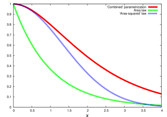
Figure 1: $\frac{1}{2^{\alpha-1}\Gamma(\alpha)}\cdot(\sigma S)^{\alpha}\cdot K_{\alpha}(\sigma S)$ at $\alpha=1.9$,   ${\rm e}^{-\sigma S}$,   ${\rm e}^{-\frac{\langle(gF_{\mu\nu}^{a})^{2}\rangle}{48N_{c}}{\,}S^{2}}$. The value $\sigma S=4$ corresponds to the radius of the contour equal to 0.51 fm.

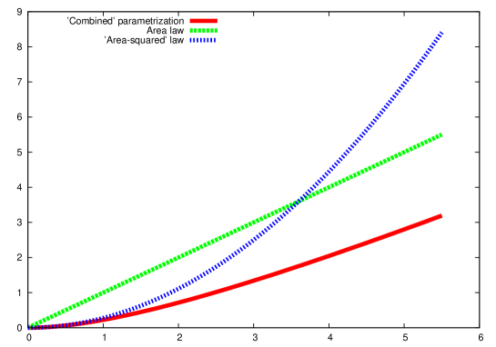
Figure 2: $-\ln\left[\frac{1}{2^{\alpha-1}\Gamma(\alpha)}\cdot(\sigma S)^{\alpha}\cdot K_{\alpha}(\sigma S)\right]$ at $\alpha=1.9$,   $\sigma S$,   $\frac{\langle(gF_{\mu\nu}^{a})^{2}\rangle}{48N_{c}}{\,}S^{2}$. The value $\sigma S=5.5$ corresponds to the radius of the contour equal to 0.6 fm. The gap between $-\ln[\cdots]$ and $\sigma S$, being $\sim\ln(\sigma S)$ at large distances, is irrelevant for the static potential.

We are now in a position to calculate $\langle\Gamma[A_{\mu}^{a},m_{n}]\rangle$, which is defined by Eq. (1) with $m$ replaced by $m_{n}$. For this purpose, we multiply the infinitesimal surface element $d\tau z_{\lambda}\dot{z}_{\rho}$ in $\Sigma_{\mu\nu}$ above by the scaling factor $Z_{n}$. Following Ref. [3], we arrive at the expression

$$\langle\Gamma[A_{\mu}^{a},m_{n}]\rangle=-2N_{\rm f}N_{c}\int_{0}^{\infty}\frac{ds}{s}{\,}{\rm e}^{-m_{n}^{2}s}\cdot\frac{\alpha(\alpha+1)(\alpha+2)}{(2\pi\tilde{\sigma}^{2})^{3}}\left(\prod\limits_{\mu<\nu}\int_{-\infty}^{+\infty}dB_{\mu\nu}\right)\frac{I(Z_{n},{\cal F}_{\mu\nu})}{\left(1+\frac{B_{\mu\nu}^{2}}{4\tilde{\sigma}^{2}}\right)^{\alpha+3}},$$ (13)

where

$$I(Z_{n},{\cal F}_{\mu\nu})=\int_{P}{\cal D}z_{\mu}\int_{A}{\cal D}\psi_{\mu}{\rm e}^{-\int_{0}^{s}d\tau\left(\frac{1}{4}\dot{z}_{\mu}^{2}+\frac{1}{2}\psi_{\mu}\dot{\psi}_{\mu}+\frac{i}{2}Z_{n}{\,}{\cal F}_{\mu\nu}z_{\mu}\dot{z}_{\nu}-iZ_{n}{\,}{\cal F}_{\mu\nu}\psi_{\mu}\psi_{\nu}\right)}$$ (14)

and ${\cal F}_{\mu\nu}\equiv\varepsilon_{\mu\nu\lambda\rho}B_{\lambda\rho}$.

The world-line integral (14) describes an infinite sum of one-loop quark diagrams, each having its own number of external lines of the auxiliary gauge field $B_{\mu\nu}$. Similarly to what was done in Ref. [3], we retain in this diagrammatic expansion only the two leading terms – the one corresponding to a free quark, which cancels out in Eq. (1), and the one corresponding to a diagram with two external lines of the gauge field. The latter yields the following expression:

$$I(Z_{n},{\cal F}_{\mu\nu})=\frac{1}{(4\pi s)^{2}}\left[\frac{4}{3}(sBZ_{n})^{2}+{\cal O}\bigl{(}(sBZ_{n})^{4}\bigr{)}\right],$$ (15)

where $B=\Bigl{(}\sum\limits_{\mu<\nu}B_{\mu\nu}^{2}\Bigr{)}^{1/2}$.

We start our analysis with the limit $n\gg 1$, where one can approximate the factor $Z_{n}$ in Eq. (15) by $S_{n}^{2}$. In the same large-$n$ limit, it is legitimate to disregard the quartic and the higher terms in the expansion (15), provided the amplitude $B$ is bounded from above as

$$B<\frac{1}{sS_{n}^{2}}=\frac{s^{2\gamma-1}}{\xi_{n}^{2}}.$$ (16)

In the last equality, we have used the explicit parametrization (10) of $S_{n}$ in terms of $s$. Now, as it was already mentioned in Introduction, the quark condensate, $\langle\bar{\psi}\psi\rangle=-\frac{\partial}{\partial m_{n}}{\,}\langle\Gamma[A_{\mu}^{a},m_{n}]\rangle$, being the quantity which characterizes the QCD vacuum, should remain $n$-independent. For this to be possible, the energy of string excitations should be largely absorbed by the constituent quark masses $m_{n}$, and it will be demonstrated below that this is what indeed happens.

An expression for the quark condensate following from Eqs. (13)-(16) reads

$$\langle\bar{\psi}\psi\rangle=-\frac{\alpha(\alpha+1)(\alpha+2)N_{\rm f}}{8\pi^{2}}\cdot m_{n}\int_{0}^{\infty}ds{\,}\frac{{\rm e}^{-m_{n}^{2}s}}{\tilde{\sigma}^{6}}{\,}S_{n}^{4}\int_{0}^{s^{2\gamma-1}/\xi_{n}^{2}}dB{\,}\frac{B^{7}}{\left(1+\frac{B^{2}}{2\tilde{\sigma}^{2}}\right)^{\alpha+3}},$$ (17)

where from now on we set $N_{c}=3$. The $B$-integration in this formula can be performed analytically, to yield

$$\langle\bar{\psi}\psi\rangle=-\frac{3N_{\rm f}}{4\pi^{2}}\cdot m_{n}\int_{0}^{\infty}ds{\,}{\rm e}^{-m_{n}^{2}s}\cdot\frac{\tilde{f}[A_{n}(s),\alpha]}{2s^{2}A_{n}(s)},$$ (18)

where

$$A_{n}(s)\equiv\frac{1}{2}\left(\frac{s^{2\gamma-1}}{\tilde{\sigma}\xi_{n}^{2}}\right)^{2},$$ (19)

while a somewhat complicated function $\tilde{f}[A,\alpha]$ was introduced in Ref. [3]. An important property of this function is that, for $\alpha\gtrsim 1$ of interest, the ratio $\tilde{f}[A,\alpha]/A$, as a function of $A$, has a maximum at $A\ll 1$, which sharpens and reaches a finite value ($\simeq 1.18$), with the further increase of $\alpha$.

In order for the quark condensate to stay finite in the small-mass limit, one should be able to represent $\frac{\tilde{f}[A_{n}(s),\alpha]}{2s^{2}A_{n}(s)}$ in the form (cf. Refs. [10, 3])

$$\frac{\tilde{f}[A_{n}(s),\alpha]}{2s^{2}A_{n}(s)}=\frac{\sigma_{0}^{3/2}}{\sqrt{s}},$$ (20)

where $\sigma_{0}$ is some parameter of dimensionality (mass)² unambiguously related to the phenomenological value of $\langle\bar{\psi}\psi\rangle$. Moreover, this representation should remain valid up to the values of the proper time such that

$$m_{n}^{2}{\,}s_{\rm max}\gtrsim 1.$$ (21)

Equation (20) can equivalently be written as

$$\frac{\tilde{f}[A_{n},\alpha]}{A_{n}}=x,~{}~{}~{}{\rm where}~{}~{}~{}x\equiv 2(\sigma_{0}s)^{3/2}.$$ (22)

Owing to the above-mentioned form of the function $\tilde{f}[A,\alpha]/A$, a solution to Eq. (22), which provides a physical decrease of $\tilde{\sigma}$ with $s$, reads $A_{n}\simeq x^{\varepsilon}$, where $\varepsilon\to 0$ for $\alpha\gtrsim 1$ of interest, and $x\lesssim 1$ (cf. Ref. [3]). Therefore, to a very good approximation, one can set in Eq. (19) $A_{n}\simeq 1$. This allows us to obtain the actual value of the power $\gamma$ in the initial Ansatz (9). To this end, we notice that, due to the energy conservation in the quark-antiquark system, a variation of the semiclassical radius $R_{n}$ of the trajectory leads to the variation $\delta m_{n}=\tilde{\sigma}{\,}\delta R_{n}$ of the constituent quark mass. Therefore, a difference between the values of the radius $R_{n}$ in the $n$-th and the 0-th states, $\delta R_{n}\equiv R_{n}-R_{0}$, reads

$$\delta R_{n}=\frac{\delta m_{n}}{\tilde{\sigma}}=\delta m_{n}\cdot\frac{\sqrt{2}\xi_{n}^{2}}{s^{2\gamma-1}},$$ (23)

where Eq. (19) has been used at the final step. Now, in order for Eqs. (9) and (23) to have the same $s$-dependence, $\gamma=1/3.$

With this value of $\gamma$ at hand, we can now calculate the correction $\delta m_{n}$ to the constituent quark mass, which is produced by the radial excitations of the quark-antiquark string. To this end, we first insert the value of $\gamma=1/3$ into Eq. (23), that leads to the following relation: $(\delta R_{n})_{\rm max}=\sqrt{2}{\,}\delta m_{n}\cdot\xi_{n,{\,}{\rm max}}^{2}{\,}s_{\rm max}^{1/3}$. Furthermore, for $\xi_{n,{\,}{\rm max}}$ in this formula we use its expression provided by Eq. (10) with $\gamma=1/3$. That yields

$$(\delta R_{n})_{\rm max}=\pi\sqrt{2}\cdot\frac{\delta m_{n}{\,}s_{\rm max}}{\sigma R_{0,{\,}{\rm max}}^{2}}\left[\sqrt{n+\frac{3}{4}}-\sqrt{\frac{3}{4}}-(\delta f_{n})_{\rm min}\right]^{2}.$$ (24)

Next, we use the approximation $\delta m_{n}{\,}s_{\rm max}\simeq 1/(\delta m_{n})_{\rm min}$, which reflects the fact that the trajectory of a maximum size (and therefore requiring the maximum proper time to be orbited) is reached when the value of the constituent quark mass is minimal. [Notice that this approximation parallels condition (21).] Substituting this approximation into Eq. (24), we arrive at the following equation:

$$(\delta m_{n})_{\rm min}\simeq\frac{\pi\sqrt{2}}{\sigma R_{0,{\,}{\rm max}}^{2}(\delta R_{n})_{\rm max}}\left[\sqrt{n+\frac{3}{4}}-\sqrt{\frac{3}{4}}-(\delta f_{n})_{\rm min}\right]^{2}.$$ (25)

In order to solve this equation, we represent it entirely in terms of $(\delta f_{n})_{\rm min}$. That can be done by virtue of the relation $(\delta m_{n})_{\rm min}=\sqrt{\pi\sigma}{\,}(\delta f_{n})_{\rm min}$, which stems from Eq. (6). As a result, we obtain the following quadratic equation:

$$(\delta f_{n})_{\rm min}+b\cdot(\delta f_{n})_{\rm min}^{1/2}-\left(\sqrt{n+\frac{3}{4}}-\sqrt{\frac{3}{4}}\right)=0,~{}~{}~{}{\rm where}~{}~{}~{}b\equiv\frac{\sigma^{3/4}R_{0,{\,}{\rm max}}(\delta R_{n})_{\rm max}^{1/2}}{(2\pi)^{1/4}}.$$ (26)

A solution to this equation yields the sought correction to the constituent quark mass:

$$(\delta m_{n})_{\rm min}=\sqrt{\pi\sigma}\cdot(\delta f_{n})_{\rm min}=\frac{\sqrt{\pi\sigma}}{4}\left[\sqrt{b^{2}+4\left(\sqrt{n+\frac{3}{4}}-\sqrt{\frac{3}{4}}\right)}-b\right]^{2}.$$ (27)

The limits of this formula at large and small $n$’s will be analyzed in the next Section.

3 The limiting cases of large and small excitations. Concluding remarks

Ignoring for a moment the effect of string-breaking, we see that the obtained $(\delta m_{n})_{\rm min}$, Eq. (27), vanishes in the limit of $b\to\infty$, which corresponds to the quark-antiquark string of an infinite length [cf. the definition of $b$ in Eq. (26)]. In reality, however, the string-breaking phenomenon imposes an upper limit on the possible values of $b$. Indeed, the upper limit for both $R_{0,{\,}{\rm max}}$ and $(\delta R_{n})_{\rm max}$ is given by $d_{\rm s.b.}/2$, where $d_{\rm s.b.}$ is the string-breaking distance. Lattice simulations and analytic studies [11] suggest for this distance the value of $d_{\rm s.b.}\simeq 1.5{\,}{\rm fm}$. Using also the phenomenological value of $\sigma\simeq(440{\,}{\rm MeV})^{2}$, we get $b\lesssim 1.37$. Therefore, we find from Eq. (27) the realistic asymptotic behavior of the constituent quark mass to be

$$(\delta m_{n})_{\rm min}\to\sqrt{\pi\sigma n}~{}~{}~{}{\rm for}~{}~{}~{}n\gg 1.$$ (28)

Comparison of this result with the initial Eqs. (4) and (5) shows that, in the large-$n$ limit, the leading contribution to the excitation energy $E_{n}$ of the quark-antiquark pair stems from the constituent quark masses. Indeed, one can perform the large-$n$ expansion of $(\delta f_{n})_{\rm min}$ given by Eq. (27), which yields $(\delta f_{n})_{\rm min}=\sqrt{n}\left[1-bn^{-1/4}+{\cal O}(n^{-1/2})\right]$. Then, inserting this expansion into the formula for $S_{n}$, Eq. (10), we obtain the leading large-$n$ behavior

$$S_{n}\bigr{|}_{s=s_{\rm max}}\to\frac{\sqrt{\pi/\sigma}}{R_{0,{\,}{\rm max}}}\cdot b\;n^{1/4},$$ (29)

which is subdominant compared to Eq. (28). Recalling Eq. (7), we conclude that

$$m_{n,{\,}{\rm min}}\sim L_{n}^{2}.$$

Thus, the constituent quark mass appears as a primary ingredient of the excitation energy of the quark-antiquark pair in the large-$n$ limit, whereas the elongation of the string plays only a secondary role. Still, we observe an increase of $S_{n}$ with $n$, which, for sufficiently large $n$’s, validates the approximation $Z_{n}\simeq S_{n}^{2}$ used after Eq. (15).

Let us now evaluate a correction to the constituent quark mass, which is associated with the $(n=1)$ excitation. We note that this excitation is developed just on top of the maximally-stretched unexcited-string configuration. For this reason, one can use for such an evaluation the above-adopted maximum values of $b=1.37$ and $R_{0,{\,}{\rm max}}=0.75{\,}{\rm fm}$, and also set $s=s_{\rm max}$. Extrapolating then Eq. (29) down to $n=1$, we get $S_{1}\equiv\left.S_{1}\right|_{s=s_{\rm max}}=1.45$. The fact that this extrapolation to $n=1$ of the initial parametrically large result of Eq. (29) leads to $S_{1}\sim 1$, signals the need to introduce some correcting numerical factor $k$. It can be defined through the relation $(kS_{1})^{2}=Z_{1}$, where again $Z_{1}=(1+S_{1})^{2}$. This equation yields the value of $k=1.69$. Next, according to Eq. (29), the multiplication of $S_{1}$ by a factor of $k$ is equivalent to the multiplication of $b$ by such a factor. This observation yields the corrected value of $b=2.32$. Inserting it into Eq. (27), we get the sought estimate for the $(n=1)$ correction to the constituent quark mass:

$$(\delta m_{1})_{\rm min}=26.0{\,}{\rm MeV}.$$

This value looks like a reasonable additive correction to the leading result, $m=460{\,}{\rm MeV}$, quoted in the Introduction.

In conclusion, we notice that excitations of the quark-antiquark pairs can in general lead to an increase of the constituent quark mass and to an elongation of the quark-antiquark string. In this talk, we have shown that, for large radial excitations $n$, the constituent quark mass grows as ${\cal O}(n^{1/2})$, while the length of the string grows only as ${\cal O}(n^{1/4})$. This result clearly means that the excitation energy of a quark-antiquark pair stems mostly from the increase of the constituent quark masses and not from string elongation. Thus, at least within the effective-action formalism, excited quark-antiquark bound states tend to have essentially the same size, irrespective of their radial excitations. This is true even if we had energy dependence for bound states different from that of Eq. (4), because that will be just another prescription for the area scaling and hence, the final qualitative result would not depend on actual details on how this scaling is obtained, but just from the fact that for a given scaling up of the area, the mass would go like the square of the string elongation, whereas the string energy would dimensionally go with $\sigma L_{n}$. Finally, such size stiffness will preclude decay channels to become large with string elongations, because they chiefly measure the size of the parent hadron and that does not change appreciably. We also emphasize that the adopted calculational method does not rely on any specific class of the string deformations (such as, e.g., the normal modes). Finally, it looks natural to apply the present approach to the description of an interesting lattice result [12] that, for quarks in the fundamental representation, the deconfinement and the chiral-symmetry-restoration temperatures are nearly the same, whereas for quarks in the adjoint representation, the chiral-symmetry-restoration temperature exceeds the deconfinement one by a factor of 8. Work in this direction is currently in progress.

- [1] For reviews, see: A. Di Giacomo, H. G. Dosch, V. I. Shevchenko and Yu. A. Simonov, Phys. Rept. 372, 319 (2002); D. Antonov, Surveys High Energ. Phys. 14, 265 (2000).
- [2] Z. Bern and D. A. Kosower, Phys. Rev. Lett. 66, 1669 (1991); Nucl. Phys. B 379, 451 (1992); M. J. Strassler, Nucl. Phys. B 385, 145 (1992); M. G. Schmidt and C. Schubert, Phys. Lett. B 318, 438 (1993); ibid. B 331, 69 (1994); for reviews, see: M. Reuter, M. G. Schmidt and C. Schubert, Annals Phys. 259, 313 (1997); C. Schubert, Phys. Rept. 355, 73 (2001).
- [3] D. Antonov and J. E. F. T. Ribeiro, Phys. Rev. D 81, 054027 (2010).
- [4] D. Antonov, H.-J. Pirner and M. G. Schmidt, Nucl. Phys. A 832, 314 (2010).
- [5] See, e.g.: N. Brambilla, P. Consoli and G. M. Prosperi, Phys. Rev. D 50, 5878 (1994); A. Yu. Dubin, A. B. Kaidalov and Yu. A. Simonov, Phys. Lett. B 323, 41 (1994); D. Antonov, Phys. Lett. B 696, 214 (2011).
- [6] H. G. Dosch and Yu. A. Simonov, Phys. Lett. B 205, 339 (1988).
- [7] N. Brambilla and A. Vairo, Phys. Rev. D 55, 3974 (1997).
- [8] See: S. Donnachie, H. G. Dosch, O. Nachtmann and P. Landshoff, Pomeron physics and QCD, Cambridge Univ. Press, 2002, and D. V. Bugg, Phys. Rept. 397, 257 (2004), for the theoretical and the experimental reviews, respectively.
- [9] M. D’Elia, A. Di Giacomo and E. Meggiolaro, Phys. Lett. B 408, 315 (1997).
- [10] T. Banks and A. Casher, Nucl. Phys. B 169, 103 (1980); J. B. Kogut, Rev. Mod. Phys. 55, 775 (1983).
- [11] C. E. Detar, O. Kaczmarek, F. Karsch and E. Lärmann, Phys. Rev. D 59, 031501 (1999); O. Kaczmarek, S. Ejiri, F. Karsch, E. Lärmann and F. Zantow, Prog. Theor. Phys. Suppl. 153, 287 (2004); D. Antonov, L. Del Debbio and A. Di Giacomo, JHEP 08, 011 (2003); D. Antonov and A. Di Giacomo, JHEP 03, 017 (2005).
- [12] F. Karsch and M. Lütgemeier, Nucl. Phys. B 550, 449 (1999).