Inhomogeneities in the universe

Abstract

Standard models of galaxy formation predict that matter distribution is statistically homogeneous and isotropic and characterized by (i) spatial homogeneity for $r<10$ Mpc/h, (ii) small-amplitude structures of relatively limited size (i.e., $r<100$) Mpc/h and (iii) anti-correlations for $r>r_{c}\approx 150$ Mpc/h (i.e., no structures of size larger than $r_{c}$). Whether or not the observed galaxy distribution is interpreted to be compatible with these predictions depend on the a-priori assumptions encoded in the statistical methods employed to characterize the data and on the a-posteriori hypotheses made to interpret the results. We present strategies to test the most common assumptions and we find evidences that, in the available samples, galaxy distribution is spatially inhomogeneous for $r<100$ Mpc/h but statistically homogeneous and isotropic. We conclude that the observed inhomogeneities pose a fundamental challenge to the standard picture of cosmology but they also represent an important opportunity which may open new directions for many cosmological puzzles.

1 Introduction

One of cornerstone of modern cosmology is represented by the observations of the three dimensional distribution of galaxies [1, 2]. In recent years the extraordinary increase of the number of redshifts has allowed us to characterize in detail galaxy structures at low redshifts (i.e., $z<0.3$) and small scales (i.e., $r<150$ Mpc/h). Many authors (see e.g., [3, 4, 5, 6, 7, 8, 9]) have concluded that the results of a statistical analysis of the data are compatible with the theoretical expectations of standard scenarios of galaxy as the Cold Dark Matter (CDM) model and its variants (i.e., the case in which the cosmological constant is non zero or LCDM). However, there are some important methodological issues which have not received the due attention [10, 11, 12, 14, 15, 16]. In particular, the critical points concern the a-priori assumptions which are usually used, without being directly tested, in the statistical analysis of the data and the a-posteriori hypotheses that are invoked to interpret the results.

Among the former, there are the assumptions of spatial homogeneity and of translational and rotational invariance (i.e., statistical homogeneity) which are built in the definition of the standard estimators of galaxy correlations [17]. While these estimators are certainly the correct ones to use when statistical and spatial homogeneity are verified, it is not simply evident that galaxy data do satisfy these properties in the available samples. It is indeed well known that galaxies are organized into a network of structures, like clusters, filaments and voids, with large fluctuations [18, 19, 20, 21, 22, 23] and it is not a-priori obvious that spatial or statistical homogeneity are satisfied in a sample of arbitrary small size.

The observed galaxy distribution is found to be inhomogeneous at small scales while, according to theoretical models it is expected to become spatially homogeneous for $r>\lambda_{0}\approx 10$ Mpc/h (see, e.g., [24]): this scale can be easily calculated by considering how the scale at which fluctuations are order of the mean evolves according to linear perturbation theory of a self-gravitating fluid[25]. The scale $\lambda_{0}$, a key theoretical prediction which must be confronted with the data, is usually determined only indirectly by using statistical methods which assume a-priori spatial homogeneity. When the given finite sample distribution is not spatially homogeneous the results of the analysis are very misleading [17]. Therefore, in order to test directly whether a distribution is spatially homogeneous it is necessary to introduce more general statistical methods than the usual ones [17, 11]. These methods consider explicitly the problem of the stability of finite sample determinations: if a statistical quantity depends on the sample size then it is affected by large fluctuations and/or by observational systematic effects; in both cases it does not represent a meaningful and useful estimator of an ensemble average property. A critical analysis of finite-sample volume averages is thus necessary to identify the subtle effects induced by spatial inhomogeneities and to distinguish them from other intervening systematic effects.

As mentioned above, a second kind of ad-hoc hypotheses are often used in the interpretation of the results of the statistical analysis. These are invoked when one finds results which are a-priori unexpected and which clearly show that some of the basic assumptions encoded in the used statistical methods are not verified in the data. Examples are galaxy evolution, luminosity bias, or selection effects due to some observational issues. It is plausible that some of these may affect the results of a statistical analysis; however, in the absence of a quantitative prediction or of an independent estimation of these effects, one must use several assumptions (e.g., specific functional behavior or arbitrary values for a set of parameters, etc.) [26, 27, 4] without any clean test of their validity. A different strategy, which, when possible, we adopt here, is to develop focussed tests to understand whether the quantitative influence of the intervening systematic effects are supported by the given data.

Theoretical models predict the matter density field properties both in the early and in the late universe. Fluctuations and correlations must have very specific properties. Firstly, the Friedmann-Robertson-Walker (FRW) geometry is derived under the assumption that matter distribution is exactly translational and rotational invariant, i.e. that the matter density is assumed to be constant in a spatial hyper-surface. On the top of the mean field one can consider statistically homogeneous and isotropic small-amplitude fluctuations [28]. These furnish the seeds of gravitational clustering which eventually give rise to the structures we observe in the present universe.

Secondly, the statistical properties of matter density fluctuations have to satisfy an important condition in order to be compatible with the FRW geometry [29, 30]. In its essence, the condition is that fluctuations in the gravitational potential induced by density fluctuations do not diverge at large scales [31, 17, 33]. This situation requires that the matter density field fluctuations must decay in the fastest possible way with scale [32]. Correspondingly the two-point correlation function becomes negative at larger scales (i.e., $r>150$ Mpc/h) which implies the absence of larger structures of tiny density fluctuations. Are the observed large scale structures and fluctuations compatible with such a scenario ?

This paper is organized as follows. In Sect.2 we briefly review the main properties of both spatially homogeneous and inhomogeneous stochastic density fields. The main features of real space correlation properties of standard cosmological density fields are presented in Sect.3. In the case of a finite-sample distribution (Sect.4) the information that can be exacted from the data is through a statistical analysis, and hence through the computation of volume averages. We discuss how to set up a strategy to analyze a point distribution in a finite volume, stressing the sequence of steps that should be considered in order to reduce as much as possible the role of a-priori assumptions encoded in the statistical analysis and to correctly interpret the meaning of the measured volume averages. The analysis of the galaxy data is presented in Sect.5. We show that galaxy distribution, at relatively low redshifts (i.e., $z<0.3$) and small scales (i.e., $r<150$ Mpc/h) is characterized by large density fluctuations which correspond to large-scale correlations. We emphasis that by using the standard statistical tools one reaches a different conclusion. This occurs because these methods are based on several important assumptions: some of them, when directly tested are not verified, while others are very strong ad-hoc hypotheses which require a detailed investigation. Finally in Sect.6 we draw our main conclusions.

2 A brief review of the main statistical properties

Before entering in the problems related to the statistical characterization in finite samples, we review the main probabilistic properties of mass density fields. This means that we consider ensemble averages or, for ergodic cases, volume averages in the infinite volume limit.

A mass density field can be represented as a stationary stochastic process that consists in extracting the value of the microscopic density function $\rho(\vec{r})$ at any point of the space. This is completely characterized by its probability density functional ${\cal P}[\rho(\vec{r})]$. This functional can be interpreted as the joint probability density function (PDF) of the random variables ${\rho}(\vec{r})$ at every point $\vec{r}$. If the functional ${\cal P}[\rho(\vec{r})]$ is invariant under spatial translations then the stochastic process is statistically homogeneous or translational invariant (stationary) [17]. When ${\cal P}[\rho(\vec{r})]$ is also invariant under spatial rotation then the density field is statistically isotropic [17].

A crucial assumption usually used, when comparing theoretical prediction to data, is that stochastic fields are required to satisfy spatial ergodicity. Let us take a generic observable ${\cal F}={\cal F}(\rho(\vec{r}_{1}),\rho(\vec{r}_{2}),...)$ function of the mass distribution $\rho(\vec{r})$ at different points in space $\vec{r}_{1},\vec{r}_{2},...\;$. Ergodicity implies that $\left<{\cal F}\right>=\overline{{\cal F}}=\lim_{V\rightarrow\infty}\overline{{\cal F}}_{V}\;,$ where the symbol $\langle...\rangle$ is for the (ensemble) average over different realizations of the stochastic process, and $\overline{{\cal F}}_{V}=\frac{1}{V}\int_{V}{\cal F}dV$ is the spatial average in a finite volume $V$ [17].

2.1 Spatially homogeneous distributions

The condition of spatial homogeneity (uniformity) is satisfied if the ensemble average density of the field $\rho_{0}=\langle\rho\rangle$ is strictly positive, i.e. for an ergodic stochastic field [17],

$$\langle\rho\rangle=\lim_{R\rightarrow\infty}\frac{1}{V(R;\vec{x_{0}})}\int_{V(R;\vec{x_{0}})}\rho(r)d^{3}r>0\;\;\forall\vec{x_{0}}\;,$$ (1)

where $R$ is the linear size of a volume $V$ with center in $\vec{x_{0}}$. Note that it is necessary to carefully test spatial homogeneity before applying the definitions given in this section to a finite sample distribution (see Sect.4). Indeed, for inhomogeneous distributions the estimation of the average density substantially differs from its asymptotic value and thus the sample estimation of $\rho_{0}$ is biased by finite size effects. Unbiased tests of spatial homogeneity can be achieved by measuring conditional properties (see below).

A distribution is spatially inhomogeneous up to a scale $\lambda_{0}$, i.e. or spatially homogeneous for $r>\lambda_{0}$, if [17]

$$\left|\frac{1}{V(R;\vec{x_{0}})}\int_{V(R;\vec{x_{0}})}d^{3}x\rho(\vec{x})-\rho_{0}\right|<\rho_{0}\;\;\forall R>\lambda_{0}\;\;,\forall\vec{x_{0}}\;.$$ (2)

This equation defines the homogeneity scale $\lambda_{0}$ which separates the strongly fluctuating regime $r<\lambda_{0}$ from the regime where fluctuations have small amplitude relative to the asymptotic average.

Let us now discuss the characterization of two-point correlation properties. The quantity $\langle\rho(\vec{r_{1}})\rho(\vec{r_{2}})\rangle dV_{1}dV_{2}$ gives the a-priori probability to find two particles simultaneously placed in the infinitesimal volumes $dV_{1},dV_{2}$ respectively around $\vec{r_{1}},\vec{r_{2}}$. The quantity

$$\langle\rho(r_{12})\rangle_{p}dV_{1}dV_{2}=\frac{\langle\rho(\vec{r_{1}})\rho(\vec{r_{2}})\rangle}{\rho_{0}}dV_{1}dV_{2}$$ (3)

gives the a-priori probability of finding two particles placed in the infinitesimal volumes $dV_{1},dV_{2}$ around $\vec{r_{1}}$ and $\vec{r_{2}}$ with the condition that the origin of the coordinates is occupied by a particle (Eq.3 is the ratio of unconditional quantities, and thus, for the roles of conditional probabilities, it defines a conditional quantity) [17].

For a stationary and spatially homogeneous distribution (i.e., $\rho_{0}>0$), we may define the reduced two-point correlation function as [17]

$$\xi(r_{12})=\frac{\langle\rho(r_{12})\rangle_{p}}{\rho_{0}}-1=\frac{\langle\rho(r_{12})\rangle}{\rho_{0}^{2}}-1\;.$$ (4)

This function characterizes two-point correlation properties of small amplitude density fluctuations. When spatial homogeneity has already been proved there are several useful information that can be extracted from $\xi(r)$, and in particular one or a few characteristic length scales. For instance, the correlation length typically corresponds to an exponential decay of $\xi(r)$ of the type $\xi(r)\sim\exp(-r/r_{c})$ [17].

The two-point correlation function defined by Eq.4 is simply related to the normalized mass variance in a volume $V(R)$ of linear size $R$ [17]

$$\sigma^{2}(R)=\frac{\langle M(R)^{2}\rangle-\langle M(R)\rangle^{2}}{\langle M(R)\rangle^{2}}=\frac{1}{V^{2}(R)}\int_{V(R)}d^{3}r_{1}\int_{V(R)}d^{3}r_{2}\xi(r_{12})\;.$$ (5)

The scale $r_{*}$ at which fluctuations are of the order of the mean, i.e. $\sigma(r_{*})=1$, is proportional to the scale $r_{0}$ at which $\xi(r_{0})=1$ and to the scale $\lambda_{0}$ defined in Eq.2.

For spatially uniform systems, when the volume $V$ in Eq.5 is a real space sphere, it is possible to proceed to the following classification for the scaling behavior of the normalized mass variance at large enough scales [31, 17]:

$$\sigma^{2}(R)\sim\left\{\begin{array}[]{ll}R^{-(3+n)}&\mbox{for }\,-3<n<1\\ R^{-(3+1)}\log R&\mbox{for }\,n=1\\ R^{-(3+1)}&\mbox{for }\,n>1\end{array}\right.\;.$$ (6)

For $-3<n<0$ (which corresponds to $\xi(r)\sim r^{-\gamma}$ with $0<\gamma=3+n<3$), mass fluctuations are super-Poisson. These are, for instance, typical of systems at the critical point of a second order phase transition [17]: there are long-range correlations and the correlation length $r_{c}$ is infinite. For $n=0$ fluctuations are Poisson-like and the system is called substantially Poisson: there are no correlations (i.e., a purely Poisson distribution) or correlations limited to small scales, i.e. of the type $\xi(r)\sim\exp(-r/r_{c})$, with a finite $r_{c}$. This behavior is typical of many common physical systems, e.g., a homogeneous gas at thermodynamic equilibrium at sufficiently high temperature. Finally for $n\geq 1$ fluctuations are sub-Poisson or super-homogeneous [31, 17] (or hyper-uniform [32]). In this case $\sigma^{2}(R)$ presents the fastest possible decay for discrete or continuous distributions [31] and the two-point correlation function has to satisfy the following global constraint

$$\int_{0}^{\infty}d^{3}r\xi(r)=0\;,$$ (7)

(see for more details Sect.3). Examples are provided by the one component plasma, a well-known system in statistical physics [34], and by a randomly shuffled lattice of particles [17, 35].

Note that any uniform stochastic process has to satisfy the following condition

$$\lim_{R\rightarrow\infty}\sigma^{2}(R)=\lim_{R\rightarrow\infty}=\frac{1}{V^{2}(R)}\int_{V(R)}d^{3}r_{1}\int_{V(R)}d^{3}r_{2}\xi(r_{12})=0$$ (8)

which implies that the average density $\rho_{0}$, in the infinite volume limit, is a well defined concept, i.e. $\rho_{0}>0$ [17]. This is a weaker condition than that required by Eq.7.

2.2 Spatially inhomogeneous distributions

A distribution is spatially inhomogeneous in the ensemble (or in the infinite volume limit) sense if $\lambda_{0}\rightarrow\infty$. For statistically homogeneous distributions, from Eq.2, we find that the ensemble average density is $\rho_{0}=0$. Thus unconditional properties are not well defined: if we consider a randomly placed finite volume in an infinite inhomogeneous distribution, it typically contains no points. Therefore only conditional properties are well defined, as for instance the average conditional density defined in Eq.3.

For a statistically homogeneous and isotropic fractal structure (where all points are alike) the average conditional mass included in a spherical volume grows as $\langle M(r)\rangle_{p}\sim r^{D}$: for $D<3$, the average conditional density presents a scaling behavior of the type [17]

$$\langle\rho(r)\rangle_{p}=\frac{\langle M(r)\rangle_{p}}{V(r)}\sim r^{D-3}\;,$$ (9)

so that $\lim_{r\rightarrow\infty}\langle\rho(r)\rangle_{p}=0$. The hypotheses underlying the derivation of the Central Limit Theorem are violated by the long-range character of spatial correlations, resulting in a PDF of fluctuations that does not follow the Gaussian function [17, 36]. On the contrary, the PDF typically displays “long tails” and some moments of the distribution may diverge [37] .

It is possible to introduce more complex inhomogeneous distributions than Eq.9, for instance the multi-fractal distributions for which the scaling properties are not described by a single exponent, but they change in different spatial locations [17]. Another simple (and different !) example is given by a distribution in which the scaling exponent in Eq.9 depends on distance, i.e. $D=D(r)<3$.

3 Statistical properties of the standard model

As discussed in the introduction, the important constraint that must be valid for any kind of matter density fluctuation field in the framework of FRW models, is represented by the condition of super-homogeneity, corresponding in cosmology to the so-called property of “scale-invariance” of the primordial fluctuations power spectrum (PS) [31]. To avoid confusion, note that in statistical physics the term “scale invariance” is used to describe the class of distributions which are invariant with respect to scale transformations. For instance, a magnetic system at the critical point of transition between the paramagnetic and ferromagnetic phase, shows a two-point correlation function which decays as a non-integrable power law, i.e. $\xi(r)\sim r^{-\gamma}$ with $0<\gamma<3$ (super-Poisson distribution in Eq.6). The meaning of “scale-invariance” in the cosmological context is therefore completely different, referring to the property that the mass variance at the horizon scale be constant (see below) [31].

3.1 Basic Properties

Matter distribution in cosmology is assumed to be a realization of a stationary stochastic point process that is also spatially uniform. In the early universe the homogeneity scale $\lambda_{0}$ is of the order of the inter-particle distance, and thus negligible, while it grows during the process of structure formation driven by gravitational clustering. The main property of primordial density fields in the early universe is that they are super-homogeneous, satisfying Eq.6 with $n=1$. This latter property was firstly hypothesized in the seventies [29, 30] and it subsequently gained in importance with the advent of inflationary models in the eighties [31].

In order to discuss this property, let us recall that the fluctuations in the early universe are taken to have Gaussian statistics and a certain PS. Since fluctuations are Gaussian, the knowledge of the PS gives a complete statistical description of the fluctuation field. In a FRW cosmology there is a fundamental characteristic length scale, the horizon scale $R_{H}(t)$ that is simply the distance light can travel from the Big Bang singularity $t=0$ until any given time $t$ in the evolution of the Universe. This scale linearly grows with time. Harrison [29] and Zeldovich [30] introduced the criterion that matter fluctuations have to satisfy on large enough scales. This is named the Harrison-Zeldovich criterion (H-Z); it can be written as [17]

$$\sigma^{2}(R=R_{H}(t))={\rm constant}.$$ (10)

This condition states that the mass variance at the horizon scale is constant: it can be expressed more conveniently in terms of the PS for which Eq.10 is equivalent to assume $P(k)\sim k$ (the H-Z PS) and that in a spatial hyper-surface $\sigma^{2}(R)\sim R^{-4}$ [31, 17].

3.2 Physical implications of super-homogeneity

In order to illustrate the physical implications of the H-Z condition, one may consider the gravitational potential fluctuations $\delta\phi(\vec{r})$, which are linked to the density fluctuations $\delta\rho(\vec{r})$ via the gravitational Poisson equation: $\nabla^{2}\delta\phi(\vec{r})=4\pi G\delta\rho(\vec{r})\,.$ From this equation, transformed into Fourier space, it follows that the PS of the gravitational potential fluctuations $P_{\phi}(k)=\left<|\delta\hat{\phi}(\vec{k})|^{2}\right>$ is related to the density PS $P(k)$ through the equation $P_{\phi}(k)\sim\frac{P(k)}{k^{4}}$. The H-Z condition, $P(k)\sim k$, corresponds therefore to $P_{\phi}(k)\propto k^{-3}$, so that the variance of the gravitational potential fluctuations, $\sigma_{\phi}^{2}(R)\approx\frac{1}{2}P_{\phi}(k)k^{3}|_{k=R^{-1}}$, is constant with $k$ [31].

The H-Z condition is a consistency constraint in the framework of FRW cosmology. Indeed, the FRW is a cosmological solution for a perfectly spatially and statistically homogeneous universe, about which fluctuations represent inhomogeneous perturbations. If density fluctuations obey to a different condition than Eq.10, and thus $n<1$ in Eq.6, then the FRW description will always break down in the past or future, as the amplitude of the perturbations become arbitrarily large or small. Thus the super-homogeneous nature of primordial density field is a fundamental property independently on the nature of dark matter. This is a very strong condition to impose, and it excludes even Poisson processes ($n=0$ in Eq.6) [31] for which fluctuations in gravitational potential diverge at large scales.

3.3 The two-point correlation function and super-homogeneity

The super-homogeneity (or H-Z) condition corresponds to the limit condition expressed by Eq.7, which represents another way to reformulate that $\lim_{k\rightarrow 0}P(k)=0$. This means that there is a fine tuned balance between small-scale positive correlations and large-scale negative anti-correlations [31, 17].

Various models of primordial density fields differ for the behavior of the PS at large wave-lengths which is determined by the specific properties hypothesized for the dark matter component. For example, in the Cold Dark Matter (CDM) scenario, where elementary non-baryonic dark matter particles have a small velocity dispersion, the PS decays as a power law $P(k)\sim k^{-2}$ at large $k$. For Hot Dark Matter (HDM) models, where the velocity dispersion is large, the PS presents an exponential decay at large $k$. However at small $k$ they both exhibit the H-Z tail $P(k)\sim k$ which is indeed the common feature of all density fields compatible with FRW models. The scale $r_{c}\approx k_{c}^{-1}$ at which the PS shows the turnover from the linear to the decaying behavior is fixed to be the size of the horizon at the time of equality between matter and radiation [42].

Correspondingly, the correlation function $\xi(r)$ of CDM (HDM) models (see Fig.1) presents the following behavior: it is positive at small scales (decaying as $\xi(r)\sim r^{-1}$ for CDM and being almost flat for HDM), it crosses zero at $r_{c}$ and then it is negative approaching zero as $-r^{-4}$ (in the region corresponding to $P(k)\sim k$) [17].

3.4 Baryonic acoustic oscillations

Let us now mention the baryon acoustic oscillations (BAO) scale [38]. The physical description which gives rise to these oscillations is based on fluid mechanics and gravity: when the temperature of the plasma was hotter than $\sim 10^{3}$ K, photons were hot enough to ionize hydrogen so that baryons and photons can be described as a single fluid. Gravity attracts and compresses this fluid into the potential wells associated with the local density fluctuations. Photon pressure resists this compression and sets up acoustic oscillations in the fluid. Regions that have reached maximal compression by recombination become hotter and hence are now visible as local positive anisotropies in the cosmic microwave background radiation (CMBR), if the different $k-$modes are assumed to have the same phase (which is the central hypothesis in this context).

For our discussion, the principal point to note is that while $k-$oscillations are de-localized, the real space correlation function $\xi(r)$ has a localized feature at the scale $r_{bao}$ corresponding to the frequency of oscillations in $k$ space. This simply reflects that the Fourier Transform of a regularly oscillating function is a localized function. Formally the scale $r_{bao}$ corresponds to a scale where a derivative of $\xi(r)$ is not continuous [17, 39].

3.5 Size of structures and characteristic scales

In summary, there are three characteristic scales in LCDM-type models (see Fig.1).

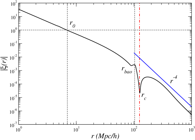
Figure 1: Schematic behavior of the two-point correlation function for the LCDM case. At small scales $r<r_{0}\approx 10$ Mpc/h (where $\xi(r_{0})=1$) non-linear gravitational clustering has changed the initial shape of $\xi(r)$. At larger scales $\xi(r)$ has been only amplified by gravitational clustering in the linear regime. For $10<r<r_{c}\approx 120$ Mpc/h the correlation is positive and with small amplitude. At larger scales it is negative and characterized by the $\xi(r)\sim-r^{-4}$ behavior. The location of $r_{bao}$ is fixed by cosmological parameters: in the example shown $r_{bao}<r_{c}$ as predicted by the “concordance model” [3].

The first is the homogeneity scale which depends on time $\lambda_{0}=\lambda_{0}(t)$, the second is the scale $r_{c}$ where $\xi(r_{c})=0$ (that is roughly proportional to the scale signing an exponential decay of $\xi(r)$) which is fixed by the initial properties of the matter density field, which also determines the third scale $r_{bao}$. When the homogeneity scale is smaller than $r_{bao},r_{c}$, these two scales are substantially unchanged by gravitational dynamics as this is in the linear regime. The rate of growth of the homogeneity scale can be simply computed by using the linear perturbation analysis of a self-gravitating fluid in an expanding universe [25]. Given the initial amplitude of fluctuations and the assumed initial PS of matter density fluctuations, under typical assumptions one finds that $\lambda_{0}(t_{now})\approx 10$ Mpc/h [24].

By characterizing the two-point correlation function of galaxy distribution we can identify three fundamental tests of standard models :

• If the homogeneity scale $\lambda_{0}$ is much larger (i.e., a factor 5-10) than $\sim 10$ Mpc/h, then there is not enough time to form non-linear large scale structures in LCDM models [11].

• If the the zero crossing scale of $\xi(r)$ is much larger than $\sim 100$ Mpc/h then there is a problem in the description of the early universe physics.

• A clear test of inflationary models is given by the detection of the negative part of the correlation function, i.e. the range of scales it behaves as $\xi(r)\sim-r^{-4}$: all models necessarily predict such a behavior .

4 Testing assumptions in the statistical methods

A number of different statistics, determined by making a volume average in a finite sample, can be used to characterize a given distribution. In addition, each statistical quantity can be measured by using different estimators. For this reason we have to set up a strategy to attack the problem if a-priori we do not know which are the properties of the given finite sample distribution. In practice, to get the correct information from the data we have to reduce as much as possible the number of a-priori assumptions used the statistical methods.

We limit our discussion to the case of interest, i.e. a set of $N$ point particles (i.e. galaxies) in a volume $V$. The microscopic number density can be simply written as $n(\vec{r})=\sum_{i}^{N}\delta^{3}(\vec{r}-\vec{r_{i}})\,,$ where $\delta^{3}(\vec{r})$ is the Dirac delta function. The statistical quantities defined in Sect.2 can be rewritten in terms of the stochastic variable

$$N_{i}(V)=\int_{V(\vec{y_{i}})}d^{3}xn(\vec{x})\,,$$ (11)

where $\vec{y_{i}}$ identifies the coordinates of the center of the volume $V$. If the center $\vec{y_{i}}$ coincides with a point particle position $\vec{r_{i}}$, then Eq.11 is a conditional quantity. Instead, if the center $\vec{y_{i}}$ can be any point of space (occupied or not by a particle) then the statistics in Eq.11 is unconditional and it is useful to compute, for instance, the mass variance defined in Eq.5.

For inhomogeneous distributions, unconditional properties are ill-defined (Sect.2) and thus we firstly analyze conditional quantities to then pass, only when spatial homogeneity has been detected inside the given sample, to consider unconditional ones. Therefore, in what follows we take as volume $V$ in Eq.11 a sphere of radius $r$ centered in a distribution point particle, i.e., we consider the stochastic variable defined by the number of points in a sphere  of radius $r$ centered on the $i^{th}$ point of the given set, i.e. $V=V(r;\vec{r_{i}})$. The PDF $P(N(r))=P(N;r)$ of the variable $N_{i}(r)$ (at fixed $r$) contains, in principle, information about moments of any order [43]. The first moment is the average conditional density and the second moment is the conditional variance [11].

However before considering the moments of the PDF we should study whether they represent statistically meaningful estimates. Indeed, in the determination of statistical properties through volume averages, one implicitly assumes that statistical quantities measured in different regions of the sample are stable, i.e., that fluctuations in different sub-regions are actually described by the same PDF. Instead, it may occur that measurements in different sub-regions show systematic (i.e., not statistical) differences, which depend, for instance, on the spatial position of the specific sub-regions. In such a case the considered statistic is not stationary in space and its whole-sample average value (i.e., any finite-sample estimation of the PDF moments) is not a meaningful descriptor. It is in this sense that it does not provide with a useful estimation of the ensemble average quantity.

4.1 Self-averaging

A simple test to determine whether there are systematic finite size effects affecting the statistical analysis in a given sample of linear size $L$ consists in studying the PDF of $N_{i}(r)$ in sub-samples of linear size $\ell<L$ placed in different spatial regions of the sample identified by their center-points $\{S_{1},...,S_{N}\}$. When, at a given scale $r<\ell$, $P(N(r),\ell;S_{i})$ is the same, modulo statistical fluctuations, in the different sub-samples, i.e.,

$$P(N(r);\ell;S_{i})\approx P(N(r);\ell;S_{j})\;\forall i\neq j\;,$$ (12)

it is possible to consider whole sample average quantities. When determinations of $P(N(r);\ell;S_{i})$ in different regions $S_{i}$ show systematic differences, then whole sample average quantities are ill defined. In general, this situation may occur because: (i) the lack of the property of translational invariance or (ii) the breaking of self-averaging property due to finite-size effects induced by large-scale structures/voids (i.e., long-range correlated fluctuations).

While the breaking of translational invariance imply the lack of self-averaging property the reverse is not true. For instance suppose that the distribution is spherically symmetric, with origin at $r_{*}$ and characterized by a smooth density profile, function of the distance from $r_{*}$ [15]. The average density in a certain volume $V$, depends on the distance of it from $r_{*}$: there is thus a systematic effect and Eq.12 is not satisfied. On the other hand when a finite sample distribution is dominated by a single or by a few structures then, even though it is translational invariant in the infinite volume limit, a statistical quantity characterizing its properties in a finite sample can be substantially affected by finite size fluctuations. For instance, a systematic effect is present when the average (conditional) density largely differs when it is measured into two disjointed volumes placed at different distances from the relevant structures (i.e., fluctuations) in the sample. In a finite sample, if structures are large enough, the measurements may differ much more than a statistical scattering . That systematic effect sometimes is refereed to as cosmic variance [22] but that is more appropriately defined as breaking of self-averaging properties [11], as the concept of variance (which involves already the computation of an average quantity) maybe without statistical meaning in the circumstances described above [11]. In general, in the range of scales in which statistical quantities give sample-dependent results, then they do not represent fair estimations of asymptotic properties of the given distribution [11].

4.2 Spatial homogeneity

The self-averaging test (Eq.12) is the first one to understand whether a distribution is spatially homogeneous or not inside a given sample. As long as the PDF $P(N,r)$ does not satisfy Eq.12 then the distribution is spatially inhomogeneous and the moments of the PDF are not useful estimators of the underlying statistical properties. Suppose that Eq.12 is found to be satisfied up to given scale $r<L$. Now we can ask the question: does the distribution become spatially homogeneous for $r<L$?

As mentioned in Sect.2, to answer to this question it is necessary to employ statistical quantities that do not require the assumption of spatial homogeneity, such as conditional ones [17, 11]. Particularly the first moment of $P(N,r)$ provides an estimation of the average conditional density defined in Eq.3, which can be simply written as

$$\overline{n(r)_{p}}=\frac{1}{M(r)}\sum_{i=1}^{M(r)}\frac{N_{i}(r)}{V(r)}=\frac{1}{M(r)}\sum_{i=1}^{M(r)}n_{i}(r)\;.$$ (13)

We recall that $N_{i}(r)$ gives the number of points in a sphere of radius $r$ centered on the $i^{th}$ point and the sum is extended to the all $M(r)$ points contained in the sample for which the sphere of radius $r$ is fully enclosed in the sample volume (this quantity is $r$ dependent because of geometrical constraints, see, e.g., [11]). Analogously to Eq.13 the estimator of the conditional variance can be written as

$$\overline{\sigma_{p}^{2}(r)}=\frac{1}{M(r)}\sum_{i=1}^{M(r)}n_{i}^{2}(r)-{\overline{n(r)_{p}}}^{2}\;.$$ (14)

In the range of scales where self-averaging properties are satisfied, one may study the scaling properties of $\overline{n(r)_{p}}$ and of $\overline{\sigma_{p}^{2}(r)}$. As long as $\overline{n(r)_{p}}$ presents a scaling behavior as a function of spatial separation $r$, as in Eq.9 with $D<3$, the distribution is spatially inhomogeneous. When $\overline{n(r)_{p}}\approx$ const. then this constant provides an estimation of the ensemble average density and the scale $\lambda_{0}$, where the transition to a constant behavior occurs, marks the homogeneity scale. Only in this latter situation it is possible to study the correlation properties of weak amplitude fluctuations. This can be achieved by considering the function $\xi(r)$ defined in Eq.4.

4.3 The two-point correlation function

Before proceeding, let us clarify some general properties of a generic statistical estimator which are particularly relevant for the two-point correlation function $\xi(r)$. As mentioned above, in a finite sample of volume $V$ we are only able to compute a statistical estimator $\overline{X_{V}}$ of an ensemble average quantity $\langle X\rangle$. The estimator is valid if

$$\lim_{V\rightarrow\infty}\overline{X_{V}}=\langle X\rangle\;.$$ (15)

If the ensemble average of the finite volume estimator satisfies

$$\langle\overline{X_{V}}\rangle=\langle X\rangle$$ (16)

the estimator is unbiased. When Eq.16 is not satisfied then there is a systematic offset which has to be carefully considered. Note that the violation of Eq.12 implies that Eq.16 is not valid as well. Finally the variance of an estimator is $\sigma_{V}^{X}=\langle\overline{X_{V}}^{2}\rangle-\langle\overline{X_{V}}\rangle^{2}$. The results given by an estimator must be discussed carefully considering its bias and its variance in any finite sample. A strategy to understand what is the effect of these features consists in changing the sample volume $V$ and study finite size effects [17, 33, 11]. This is crucially important for the two-point correlation function $\xi(r)$ as any estimator $\overline{\xi(r)}$ is generally biased, i.e. it does not satisfy Eq.16 [33, 44]. This occurs because the estimation of the sample density is biased when correlations extend over the whole sample size, or beyond it. Indeed, the most common estimator of the average density is

$$\overline{n}=\frac{N}{V}\;,$$ (17)

where $N$ is the number of points in a sample of volume $V$. It is simple to show that its ensemble average value can be written as [33]

$$\langle\overline{n}\rangle=\langle n\rangle\left(1+\frac{1}{V}\int_{V}d^{3}r\xi(r)\right)\;.$$ (18)

Therefore only when $\xi(r)=0$ (i.e., for a Poisson distribution), Eq.17 is an unbiased estimator of the ensemble average density: otherwise the bias is determined by the integral of the ensemble average correlation function over the volume $V$.

The most simple estimator of $\xi(r)$ is the Full-Shell (FS) estimator [33] that can be simply written, by following the definition given in Eq.4, as

$$\overline{\xi(r)}=\frac{\overline{(n(r))_{p}}}{\overline{n}}-1\,,$$ (19)

where $\overline{(n(r))_{p}}$ is the estimator of the conditional density in spherical shells rather than in spheres as for the case of Eq.13. Suppose that in a spherical sample of radius $R_{s}$, to estimate the sample density, instead of Eq.17, we use the estimator

$$\overline{n}=\frac{3}{4\pi R_{s}^{3}}\int_{0}^{R_{s}}\overline{(n(r))_{p}}4\pi r^{2}dr\;.$$ (20)

Then, by construction the estimator defined in Eq.19 must satisfies the following integral constraint

$$\int_{0}^{R_{s}}\overline{\xi(r)}r^{2}dr=0\;.$$ (21)

This condition is satisfied independently of the functional shape of the underlying correlation function $\xi(r)$. Thus the integral constraint for the FS estimator does not simply introduce an offset, but it causes a change in the shape of $\overline{\xi(r)}$ for $r\rightarrow R_{s}$ . Other choices of the sample density estimator [33, 44] and/or of the correlation function introduce distortions similar to that in Eq.21.

In order to show the effect of the integral constraint for the FS estimator, let us rewrite the ensemble average value of the FS estimator (i.e., Eq.19) in terms of the ensemble average two-point correlation function

$$\langle\overline{\xi(r)}\rangle=\frac{1+\xi(r)}{1+\frac{3}{R_{s}^{3}}\int_{0}^{R_{s}}\xi(r)r^{2}dr}-1\;.$$ (22)

By writing Eq.22 we assume that the stochastic noise is negligible, which, of course, is not a good approximation at any scale. However in this way we may be able to single out the effect of the integral constraint for the FS estimator. From Eq.22 it is clear that this estimator is biased, as it does not satisfy Eq.16 but only Eq.15.

As an illustrative example, let us now consider the case in which the theoretical $\xi(r)$ is a given by the LCDM model. The (ensemble average) estimator given by Eq.22, in spherical samples of different radius $R_{s}$, is shown in Fig.2. One may notice that for $R_{s}>r_{c}$ the zero point of $\overline{\xi(r)}$ remains stable, while when $R_{s}<r_{c}$ it linearly grows with $R_{s}$. The negative tail continues to be non-linearly distorted even when $R_{s}>r_{c}$. For instance, when $R_{s}\approx 600$ Mpc/h we are not able to detect the $\xi(r)\sim-r^{-4}$ tail that becomes marginally visible only when $R_{s}>1000$ Mpc/h.

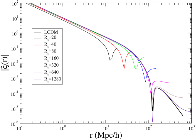
Figure 2: Absolute value of the estimation of the correlation function of the LCDM model with the integral constraint described by Eq.22. The tick solid line represents the theoretical model. The zero crossing scale correspond to the cusp ( Adapted from [33]).

Thus the stability of the zero-point crossing scale should be the first problem to be considered in the analysis of $\overline{\xi(r)}$, clearly, once spatial homogeneity has been already proved.

5 Results in the data

We briefly review the main results obtained by analyzing several samples of the Sloan Digital Sky Survey (SDSS) [10, 12, 11, 36, 15] and of the Two degree Field Galaxy Redshift Survey (2dFGRS) [45, 13, 14]. In both catalogues we selected, in the angular coordinates, a sky region such that (i) it does not overlap with the irregular edges of the survey mask and (ii) it covers a contiguous sky area. We computed the metric distance $R(z;\Omega_{m},\Omega_{\Lambda})$ from the redshift $z$ by using the cosmological parameters $\Omega_{m}=0.25$ and $\Omega_{\Lambda}=0.75$.

The SDSS catalogue includes two different galaxy samples constructing by using different selection criteria: the main-galaxy (MG) sample and the Luminous Red Galaxy (LRG) sample. In particular, the MG sample is a flux limited catalogue with apparent magnitude $m_{r}<17.77$ [46], while the LRG sample was constructed to be volume-limited (VL) [47]. A sample is flux limited when it contains all galaxies brighter than a certain apparent flux $f_{min}$. There is an obvious selection effect in that it contains intrinsically faint objects only when these are located relatively close to the observer, while it contains intrinsically bright galaxies located in wide range of distances [6]. For this reason one constructs a volume limited (VL) sample by imposing a cut in absolute luminosity $L_{min}$ and by computing the corresponding cut in distance $r_{max}\approx\sqrt{L_{min}/(4\pi f_{min})}$, so that all galaxies with $L>L_{min}$, located at distances $r<r_{max}$, have flux $f>f_{min}$, and are thus included in the sample. By choosing different cuts in absolute luminosity one obtains several VL samples (with different $L_{min},r_{max}$). Note that we use magnitudes instead of luminosities and that the absolute magnitude must be computed from the redshift by taking into account both the assumptions on the cosmology (i.e. the cosmological parameters, which very weakly perturb the final results given the low redshifts involved, i.e., $z<0.2$) and the K-corrections (which are measured in the SDSS case).

For the MG sample we used standard K-corrections from the VAGC data [48]: we have tested that our main results do not depend significantly on K-corrections and/or evolutionary corrections [11]. The MG sample angular region we consider is limited, in the SDSS internal angular coordinates, by $-33.5^{\circ}\leq\eta\leq 36.0^{\circ}$ and $-48.0^{\circ}\leq\lambda\leq 51.5^{\circ}$: the resulting solid angle is $\Omega=1.85$ sr. For the LRG sample, we exclude redshifts $z>0.36$ and $z<0.16$ (where the catalogue is known be incomplete [46, 4]), so that the distance limits are: $R_{min}=465$ Mpc/h and $R_{max}=1002$ Mpc/h. The limits in R.A $\alpha$ and Dec. $\delta$ considered are: $\alpha\in[130^{\circ},240^{\circ}]$ and $\delta\in[0^{\circ},50^{\circ}]$. The absolute magnitude is constrained in the range $M\in[-23.2,-21.2]$. With these limits we find $N=41833$ galaxies covering a solid angle $\Omega=1.471$ sr [49]. Finally for 2dFGRS, to avoid the effect of the irregular edges of the survey we selected two rectangular regions whose limits are [14]: in southern galactic cap (SGC) ($-33^{\circ}<\delta<-24^{\circ}$, $-32^{\circ}<\alpha<52^{\circ}$), and in northern galactic cap (NGC) ($-4^{\circ}<\delta<2^{\circ}$, $150^{\circ}<\alpha<210^{\circ}$); we determined absolute magnitudes $M$ using K-corrections from [50, 14].

5.1 Redshift selection function

In order to have a simple picture of the redshift distribution in a magnitude limited sample, we report Fig.3 galaxy counts as a function of the radial distance, in bins of thickness 10 Mpc/h, in the northern and southern part of the 2dFGRS [14, 13].

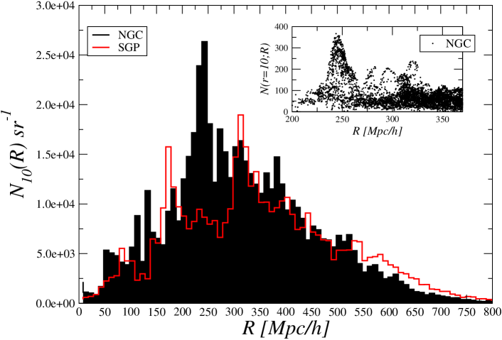
Figure 3: Radial density per unit solid angle in bins of thickness 10 Mpc/h in the northern (NGC) and souther (SGC) part of the 2dFGRS magnitude limited sample. There is a large structure at $\sim 240$ Mpc/h. In the inset panel it is shown the distribution of $N_{i}(r;R)$ for $r=10$Mpc/h in a VL sample in the NGC. (Adapted from [14]).

One may notice that a sequence of structures and voids is clearly visible, but there is an overall trend (a rise, a peak and then a decrease of the density) which is determined by a luminosity selection effect. Indeed, $n(R)$ in a flux limited sample is usually called redshift selection function, as it is determined by both the redshift distribution and by the luminosity selection criteria of the survey. It is thus not easy, by this kind of analysis, to determine, even at a first approximation, the main properties of the galaxy distribution in the samples. Nevertheless, one may readily compute that there is a $\sim 30\%$ of difference in the sample density between the northern and the southern part of the catalogue: one needs to refine the analysis to clarify its significance. Note that large scale $\sim 30\%$ fluctuations are not uncommon. For instance, fluctuations have been found in galaxy redshift and magnitude counts that are close to $50\%$ occurring on $\sim 100$ Mpc/h scales [18, 19, 20, 21].

5.2 Radial counts

A more direct information about the value of the density in a VL sample, is provided by the number counts of galaxies as a function of radial distance $n(R)$ in a VL sample. For a spatially homogeneous distribution $n(R)$ should be constant while, for a fractal distribution it should exhibit a power-law decay, even though large fluctuations are expected to occur given that this not an average quantity [51].

Figure 4: Two different slices of the same SDSS MG VL sample. Both slices cover an angular region of $100^{\circ}\times 10^{\circ}$, but in differnt directions.

In the SDSS MG VL samples, at small enough scales, $n(R)$ (see the left panel of Fig.5) shows a fluctuating behavior with peaks corresponding to the main structures in the galaxy distribution [11]. At larger scales $n(R)$ increases by a factor 3 from $R\approx 300$ Mpc/h to $R\approx 600$ Mpc/h. Thus there is no range of scales where one may approximate $n(R)$ with a constant behavior. The open question is whether the growth of $n(R)$ for $R>300$ Mpc/h is induced by structures and/or by observational selection effect in data: in principle, both are possible. For instance in [27] it is argued that a substantial galaxy evolution causes that growth, while in [11] it is discussed that structures certainly contribute to the observed a behavior. (Note that in mock catalogues drawn from cosmological N-body simulations one measures an almost constant density [11, 14]).

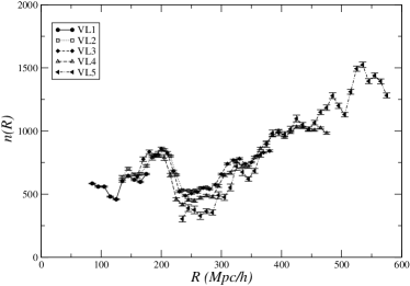
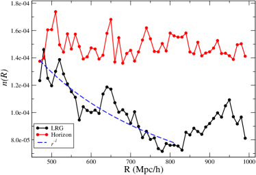
Figure 5: Left panel: Radial density in the volume limited samples of the MG catalogue. Note the amplitude of $n(R)$ for the MG VL samples has been normalized by taking into account the different selection in luminosity in the different samples ( Adapted from [11]). Right Panel: The same for the LRG sample and for a mock sample extracted from the Horizon simulations [52] (units are in (Mpc/h)^-3). The blue dashed line decays as $r^{-1}$ and it is plotted as reference. ( Adapted from [49]).

Given that, by construction, also the LRG sample should be VL [53, 7, 4] the behavior of $n(R)$ is expected to be constant if galaxy distribution is close to uniform (up to Poisson noise and radial clustering). It is instead observed that the LRG sample $n(R)$ shows an irregular and not constant behavior (see the right panel of Fig.5) rather different from that found in the MG sample. Indeed, there are two main features: (i) a negative slope between $400$ Mpc/h $<r<$ 800 Mpc/h (i.e., $0.16<z<0.28$) and (ii) a positive slope up to a local peak at $r\sim 950$ Mpc/h (i.e., $z\sim 0.34$). Note that if $n(R)$ were constant we would expect a behavior similar to the one shown by the mock sample extracted from the Horizon simulation [52] (see Fig.5) [49].

An explanation that it is usually given to interpret the behavior of $n(R)$ [7, 4], is that the LRG sample is “quasi” VL, precisely because it does not show a constant $n(R)$. Thus, the unexpected trends and features of $n(R)$ are absorbed in the properties of the so-called “the survey selection function”, which is unknown a priori, but that is defined a posteriori as the difference between an almost constant $n(R)$ and the behavior observed. This explanation is unsatisfactory as it is given a posteriori and no independent tests have been provided to corroborate the hypothesis that an important observational selection effect occurs in the data, other than the behavior of $n(R)$ itself. A different possibility is that the behavior of $n(R)$ is determined, at least partially, by intrinsic fluctuations in the distribution of galaxies and not by selection effects.

Note that, by addressing the behavior of $n(R)$ to unknown selection effects, it is implicitly assumed that more than the $20\%$ of the total galaxies have not be measured for observational problems [49]. This looks improbable [53] although a more careful investigation of the problem must be addressed. Note also that the deficit of galaxies would not be explained by a smooth redshift-dependent effect, rather the selection must be strongly redshift dependent as the behavior of $n(R)$ is not monotonic. These facts point, but do not proof, toward an origin of the $n(R)$ behavior due to the intrinsic fluctuations in the galaxy distribution.

5.3 Test on self-averaging properties

Galaxy counts provide only a rough analysis of fluctuations as one is unable to compute a truly volume average quantity. In addition galaxy counts sample different scales differently as the volume in the different redshift bins is not the same. The analysis of the stochastic variable represented by the number of points in spheres $N_{i}(r)$ an help to overcome these problems, as it is possible to construct volume averages and because it is computed in a simple real sphere sphere. (See an example in the inset panel of Fig.3).

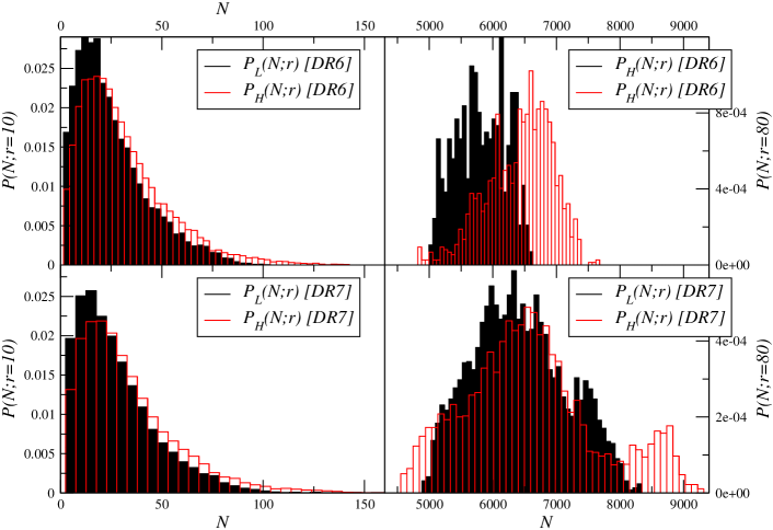
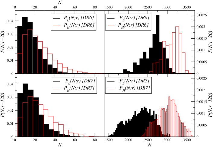
Figure 6: Upper Panels: PDF of the counts in spheres in the sample defined by $R\in[125,400]$ Mpc/h and $M\in[-20.5,-22.2]$ in the DR6 and DR7 data, for two different values of the sphere radii $r=10$ Mpc/h and $r=80$ Mpc/h. Lower Panels: The same but for the sample defined by $R\in[200,600]$ Mpc/h and $M\in[-21.6,-22.8]$ and for $r=20,120$ Mpc/h. (Adapted from [15]).

Let us thus pass to the self-averaging test described in Sect.4.1. To this aim we divide the sample into two non-overlapping regions of equal volume, one at low (L) and the other at high (H) redshifts. We then measure the PDF $P_{L}(N;r)$ and $P_{H}(N;r)$ in the two volumes ( see [15] for more details). Given that the number of independent points is not very large at large scales (i.e., $M(r)$ in Eq.13 not very larger than $\sim 10^{4}$), in order to improve the statistics especially for large sphere radii, we allow a partial overlapping between the two sub-samples, so that galaxies in the L (H) sub-sample count also galaxies in the H (L) sub-sample. This overlapping clearly can only smooth out differences between $P_{L}(N;r)$ and $P_{H}(N;r)$.

We first consider two SDSS MG VL samples from the data release 6 (DR6) [11] and then from the DR7 [15]. In a first case (upper - left panels of Fig.6), at small scales ($r=10$ Mpc/h), the distribution is self-averaging (i.e., the PDF is statistically the same) both in the DR6 sample (that covers a solid angle $\Omega_{DR6}=0.94$ sr) than in the DR7 sample ($\Omega_{DR7}=1.85$ sr $\approx 2\times\Omega_{DR6}$ sr). Instead, for larger sphere radii i.e., $r=80$ Mpc/h, (bottom - right panels of Fig.6) in the DR6 sample, the two PDF show clearly a systematic difference. Not only the peaks do not coincide, but the overall shape of the PDF is not smooth displaying a different shape. Instead, for the sample extracted from DR7, the two determinations of the PDF are in good agreement (within statistical fluctuations). We conclude that in DR6 for $r=80$ Mpc/h there are large density fluctuations which are not self-averaging because of the limited sample volume [11, 15]. They are instead self-averaging in DR7 because the volume is increased by a factor two.

For the other sample we consider, which include mainly bright galaxies, the breaking of self-averaging properties occurs only for large $r$, both in the DR6 and in the DR7 samples. As mentioned above, radial distance-dependent selections, like galaxy evolution [27], could in principle give an effect in the same direction if they tend to increase the number density with redshift. However this would not change the main conclusion that, on large enough scales, self-averaging is broken. Note that in the SDSS samples for small values of $r$ the PDF is found to be statistically stable in different sub-regions of a given sample. For this reason we do not interpret the lack of self-averaging properties as due to a “local hole” around us: this would affect all samples and all scales, which is indeed not the case [15]. Because of these large fluctuations in the galaxy density field, self-averaging properties are well-defined only in a limited range of scales where it is then statistically meaningful to measure whole-sample average quantities [11, 36, 15].

For the LRG sample (see Fig.7) one may note that for $r=50$ Mpc/h the determinations in the two are separate parts of the sample much closer than for lager sphere radii. Indeed, fro $r>100$ Mpc/h there is actually a noticeable difference in the whole shape of the PDF. The fact that $P_{H}(N;r)$ is shifted toward smaller values than $P_{L}(N;r)$ is related to the decaying behavior of the redshift counts (see Fig.5): most of the galaxies at low redshifts see a relatively larger local density than the galaxies at higher redshift.

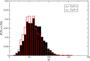
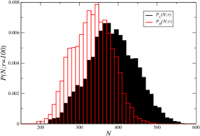
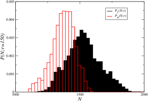
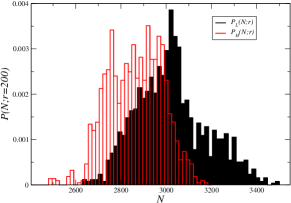
Figure 7: Upper Left Panel: PDF for $r=50$ Mpc/h in the LRG sample ( Adapted from [49]).

In summary, due the breaking of self-averaging properties in the different samples for $r<150$ Mpc/h we conclude that there is no evidence for a crossover to spatial uniformity.

5.4 Probability density function and its moments

We can refine the analysis by characterizing the shape of the PDF and the scaling of its moments. In particular, in the range of scales where self-averaging properties are found to be satisfied, we can further characterize the shape of the PDF and the scaling of its moments, particularly the first moment, the behavior of the average conditional density (Eq.13) whose behavior is presented in Fig.8. In brief, it decays approximately as $r^{-1}$ up to $\approx 20$ Mpc/h where the decay changes to $\overline{n(r)}\approx 0.011\times r^{-0.29}$  . Moreover, the density $\overline{n(r)}$ does not saturate to up to $\sim 100$ Mpc/h, i.e., up to the largest scales probed in this sample where self-averaging properties have been tested to hold. In Fig.8 it is also shown the behavior of $\overline{n(r)}$ into two non-overlapping regions of equal volume: these behaviors show the typical fluctuations affecting the estimation of this quantity.

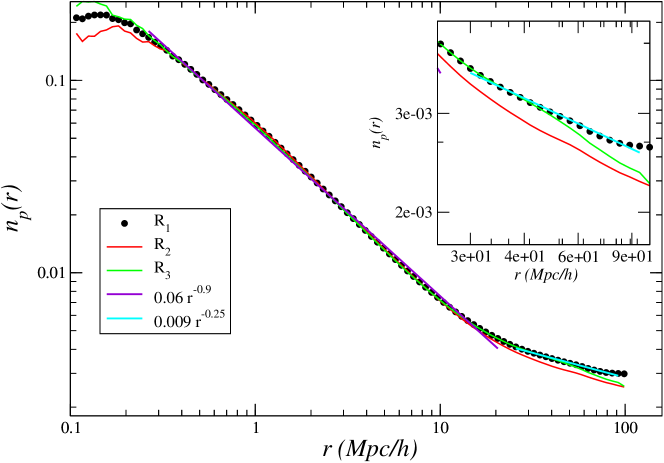
Figure 8: Conditional average density $\overline{n}(r)$ of galaxies as a function of radius ($R_{1}$). Note the change of slope at $\approx 20$ Mpc/h and note also that there is no flattening up to $\approx 100$ Mpc/h (in the inset panel it is shown a zoom at large scales). The statistical significance of the last few points at the largest scales is weaker (see text). The behavior of $\overline{n(r)}$ in two non-overlapping and equal volume regions, named $R_{2}$ and $R_{3}$, is also plotted.

The scaling behavior of the conditional density implies that galaxy structures are characterized by non-trivial correlations for scales up to $r\approx 100$ Mpc/h, without a crossover towards spatial homogeneity.

To probe the whole distribution of the conditional density $n_{i}(r)$, we fitted the measured PDF with Gumbel distribution via its two parameters $\alpha$ and $\beta$ [36]. The Gumbel distribution is one of the three extreme value distribution [54, 55]. It describes the distribution of the largest values of a random variable from a density function with faster than algebraic (say exponential) decay. The Gumbel distribution’s PDF is given by

$$P(y)=\frac{1}{\beta}\exp\left[-\frac{y-\alpha}{\beta}-\exp\left(-\frac{y-\alpha}{\beta}\right)\right]\;.$$ (23)

The mean and the variance of the Gumbel distribution (Eq.23) is $\mu=\alpha+\gamma\beta,\quad\sigma^{2}=(\beta\pi)^{2}/6$ where $\gamma=0.5772\dots$ is the Euler constant.

One of our best fit for the PDF is obtained for $r=20$ Mpc/h (see Fig. 9). At larger scales the fit get worst, but the Gumbel function remains a good fit even for $r=110$ Mpc/h. Given that the main source of uncertainty is, as discussed, finite volume systematic effects, it is not simple to determine the statistical significance of the Gumbel fit as systematic errors are larger than statistical ones.

The fact that the PDF is clearly asymmetric, and well-fitted by a Gumbel function, provides an additional evidence that correlations are long-range. Indeed, due to the Central Limit Theorem, all homogeneous point distributions with short-range correlations lead to Gaussian fluctuations [17]. It was recently conjectured [56] that only three types of distributions appear to describe fluctuations of global observables at criticality. In particular, when the global observable depends weakly on the system size (e.g., logarithmically), the corresponding distribution should be a (generalized) Gumbel [36].

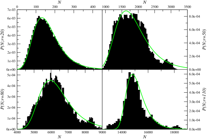
Figure 9: PDF for $r=20,50,80,100$ Mpc/h. The solid line corresponds to the best fit with a Gumbel distribution.

5.5 Two-point correlation analysis

When one determines the standard two-point correlation function one makes implicitly the assumptions that, inside a given sample the distribution is: (i) self-averaging and (ii) spatially uniform. The first assumption is used when one computes whole sample average quantities. The second is employed when supposing that the estimation of the sample density gives a fairly good estimation of the ensemble average density. When one of these assumptions, or both, is not verified then the interpretation of the results given by the determinations of the standard two-point correlation function must be reconsidered with great care.

To show how non self-averaging fluctuations inside a given sample bias the $\xi(r)$ analysis, we consider the estimator

$$\overline{\xi(r)}+1=\overline{\xi(r;R,\Delta R)}+1=\overline{n(r,\Delta r)_{p}}\cdot\frac{V(r^{*})}{\overline{N(r^{*};R,\Delta R)}}\,,$$ (24)

where the second ratio on the r.h.s. is now the density of points in spheres of radius $r^{*}$ averaged over the galaxies lying in a shell of thickness $\Delta R$ around the radial distance $R$. If the distribution is homogeneous, i.e., $r^{*}>\lambda_{0}$, and statistically stationary, Eq.24 should be (statistically) independent on the range of radial distances $(R,\Delta R)$ chosen. The two-point correlation function is defined as a ratio between the average conditional density and the sample average density: if both vary in the same way when the radial distance is changed, then its amplitude remains nearly constant. This however does not imply that the amplitude of $\overline{\xi(r)}$ is meaningful, as it can happen that the density estimated in sub-volumes of size $r^{*}$ show large fluctuations and so the average conditional density, and this occurring with a radial-distance dependence. The $\overline{\xi(r)}$ analysis gives a meaningful estimate of the amplitude of fluctuations, only if this amplitude remains stable by changing the relative position of the sub-volumes of size $r^{*}$ used to estimate the average conditional density and the sample average density. This is achieved by using the estimator in Eq.24. While standard estimators [57, 44, 33] are not able to test for such an effect, as the main contributions for both the conditional density and the sample average density come from the same part of the sample (typically the far-away part where the volume is larger). We find large variations in the amplitude of $\overline{\xi(r)}$ in the SDSS MG VL samples (see the left panel of Fig.10).

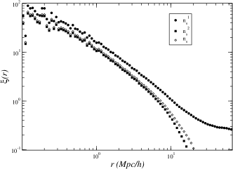
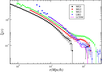
Figure 10: Left panel: The two-point correlation function in a MG-VL sample estimated by Eq.24: the sample average density is computed in spheres of radius $r^{*}=60$ Mpc/h and considering all center-points lying in a bin of thickness $\Delta R=50$ Mpc/h cantered at different radial distance $R$: $R_{1}=250$ Mpc/h ($n_{s}^{1}$) and $R_{2}=350$ Mpc/h ($n_{s}^{2}$). The case in which we have used the estimation of the sample average $N/V$ ($n_{s}$) is also shown and it agrees with the FS estimator (adapted from [11]). Right Panel: The Landy and Szalay [57] estimator of $\xi(r)$ in various MG-VL sample and in a LRG sample of the SDSS. The most evident feature is the finite-size dependence of both the amplitude and the zero-crossing (adapted from [16]). The solid line is a LCDM model.

This is simply an artifact generated by the large density fluctuations on scales of the order of the sample sizes. The results that the estimator of $\xi(r)$ has nearly the same amplitude in different samples, e.g., [58, 59, 60, 61, 7, 8, 9], despite the large fluctuations of $N_{i}(r;R)$, are simply explained by the fact that $\overline{\xi(r)}$ is a ratio between the average conditional density and the sample average density: both vary in the same way when the radial distance is changed and thus the amplitude is nearly constant.

In the right panel of Fig.10 it is plotted the behavior of $\overline{\xi(r)}$ in samples of different size. This clearly show that there is a finite-size dependence of both the amplitude of the correlation function and of the zero-crossing scale. Therefore the estimator of $\xi(r)$ is biased by volume-dependent systematic effects that make the detection of correlation amplitude only an estimate of their lower limit [16]. A similar conclusion was reached by [62], i.e. that when corrections for possible systematics are taken into account the correlation function may not be consistent with as high amplitude a peak as claimed by [3]. To clarify this issue, as discussed above, it is necessary to consider the set of tests for statistical and spatial homogeneity discussed above.

Instead of investigating the origin of the fluctuating behavior of $n(R)$, some authors [4] focused their attention on the effect of the radial counts on the determination of the two-point correlation function. In particular, they proposed mainly two different tests to study what is the effect of $n(R)$ on the determination of $\overline{\xi(r)}$. The first test consists in taking a mock LRG sample, constructed from a cosmological N-body simulation of the LCDM model, and by applying a redshift selection which randomly excludes points in such a way that the resulting distribution has the same $n(R)$ of the real sample. Then one can compare $\xi(r)$ obtained in the original mock and in redshift-sampled mock. [4] find that there is a good agreement between the two. This shows that the particular kind of redshift-dependent random sampling considered for the given distribution, does not alter the determination of the correlation function. Alternatively we may conclude that, under the assumption that the observed LRG sample is a realization of a mock LCDM simulation, the $n(R)$ does not affect the result. However, if we want to test whether the LRG sample has the same statistical properties of the mock catalogue, we cannot clearly proof (or disproof) this hypothesis by assuming a priori that this is true.

In other words, standard analyses ask directly the question of whether the data are compatible with a given model, by considering only a few statistical measurements. As it was shown by [5] the LRG correlation function does not pass the null hypothesis, i.e. it are compatible with zero signal, implying that the volume of current galaxy samples is not large enough to claim that the BAO scale is detected. In addition, by assuming that the galaxy correlations are modelled by a LCDM model, one may find that the data allow to constrain the position of the BAO scale. In our view this approach is too narrow: in evaluating whether a model is consistent with the data, one should show that at least the main statistical properties of the model are indeed consistent with the data. As discussed above, a number of different properties can be considered, which are useful to test the assumptions of (i) self-averaging and (ii) spatial homogeneity. When, inside the given sample, the assumption (i) and/or (ii) are/is violated then the compatibility test of the data with a LCDM model is not consistent with the properties of the data themselves.

6 Conclusion

The statistical characterization of galaxy structures presents a number of subtle problems. These are associated both with the a-priori assumptions which are encoded in the statistical methods used in the measurements of galaxy correlations and in the a-posteriori hypotheses that are invoked to explain certain measured behaviors. These latter include for example, luminosity bias, galaxy evolution, observational selection effects, etc. Therefore it is necessary to introduce direct tests to understand both whether the a-priori assumptions are compatible with the data and whether it is justified to introduce a-posteriori untested, but plausible, hypotheses to interpret the results of the data analysis. For instance, the analysis of the simple counts as a function of distance, in the SDSS samples, shows clearly that the observed behavior is incompatible with model predictions, i.e., spatial homogeneity. As mentioned above, one may assume that the differences between the model and the observations are due to selection effects. Then this becomes clearly the most important assumption in the data analysis that must be stressed clearly and explicitly. In addition, one must consider whether there is an independent way to study selection effects in the data.

On the basis of the results have presented, aiming to directly test whether spatial and statistical homogeneity are verified inside the available samples we conclude that galaxy distribution is characterized by structures of large spatial extension. Given that we are unable to find a crossover towards homogeneity, the amplitude of these structures remain undetermined and their main characteristic is represented by the scaling behavior of their relevant statistical properties. In particular, we discussed that the average conditional density presents a scaling behavior of the type $\sim r^{-\gamma}$ with $\gamma\approx-1$ up to $\sim 20$ Mpc/h followed by a $\gamma\approx-0.3$ behavior up to $\sim 100$ Mpc/h. Correspondingly the probability density function (PDF) of galaxy (conditional) counts in spheres shows a relatively long tail: it is well fitted by the Gumbel function instead than by the Gaussian function, as it is generally expected for spatially homogeneous, short range correlated, density fields.

The statistical tests introduced here can thus provide direct observational evidences, at small scales and low redshifts (when $z\ll 1$ we can neglect the important complications of evolving observations onto a spatial surface for which we need a specific cosmological model) of the basic assumptions used in the derivation of the FRW models, i.e. spatial and statistical homogeneity. In this respect it is worthing to further clarify the subtle difference between these two concepts [15]. The concordance model of the universe combines three fundamental assumptions: (i) Einstein’s field equations to determine the dynamics of space-time. (ii) Statistical homogeneity and isotropy, i.e., that “the Earth is not in a central, specially favored position” [64, 65]. This requirement can be though to be the Copernican Principle which is a fundamental principle because one wants to avoid any special point or direction. (iii) Spatial homogeneity: this requirement is not a fundamental one as (ii) but plays the crucial role of simplifying the solutions of the Einstein’s field equations.

The Cosmological Principle is usually meant to include both the requirement of statistical homogeneity and isotropy and of spatial homogeneity: these assumptions are often simply summarized in the requirement that the universe is homogeneous and isotropic. However one must bear in mind the fact that the universe looks the same, at least in a statistical sense, in all directions and that all observers are alike does not imply spatial homogeneity of matter distribution. It is however this latter condition that allows us to treat, above a certain scale, the density field as a smooth function, a fundamental hypothesis used in the derivation of the FRW metric.

We have shown that galaxy distribution in different samples of the SDSS is compatible with the assumption that this is transitionally invariant, i.e. it satisfies the requirement of the Copernican Principle that there are no spacial points or directions. On the other hand, we found that there are no clear evidences of spatial homogeneity up to scales of the order of the samples sizes, i.e. $\sim 100$ Mpc/h. This implies that galaxy distribution is not compatible with the stronger assumption of spatial homogeneity, encoded in the Cosmological Principle. In addition, at the largest scales probed by these samples (i.e., $r\approx 150$ Mpc/h) we found evidences for the breaking of self-averaging properties, i.e. that the distribution is not statistically homogeneous. Forthcoming redshift surveys will allow us to clarify whether on such large scales galaxy distribution is still inhomogeneous but statistically stationary, or whether the evidences for the breaking of spatial translational invariance found in the SDSS samples were due to selection effects in the data.

We note an interesting connection between spatial inhomogeneities and large scale flows which can be hypothesized by assuming that the gravitational fluctuations in the galaxy distribution reflect those in the whole matter distribution, and that peculiar velocities and accelerations are simply correlated. Peculiar velocities provide an important dynamical information as they are related to the large scale matter distribution. By studying their local amplitudes and directions, these velocities allow us, in principle, to probe deeper, or hidden part, of the Universe. The peculiar velocities are indeed directly sensitive to the total matter content, through its gravitational effects, and not only to the luminous matter distribution. However, their direct observation through distance measurements remains a difficult task. Recently, there have been published a growing number of observations of large-scale galaxy coherent motions which are at odds with standard cosmological models [68, 67, 69, 70].

It is possible to consider the PDF of gravitational force fluctuations generated by source field represented by galaxies, and test whether it converges to an asymptotic shape within sample volumes. In several SDSS sample we find that density fluctuations at the largest scales probed, i.e. $r\approx 100$ Mpc/h, still significantly contribute to the amplitude of the gravitational force [66]. Under the hypotheses mentioned above we may conclude that that large-scale fluctuations in the galaxy density field can be the source of the large scale flows recently observed.

From the theoretical point of view, it is then necessary to understand how to treat inhomogeneities in the framework of General Relativity  [65, 71, 72, 73, 74, 75, 76, 77]. To this aim one needs to carefully consider the information that can be obtained from the data. At the moment it is not possible to get some statistical information for large redshifts ($z\approx 1$), but the characterization of relatively small scales properties (i.e., $r<200$ Mpc/h) is getting more and more accurate. According to FRW models the linearity of Hubble law is a consequence of the homogeneity of the matter distribution. Modern data show a good linear Hubble law even for nearby galaxies ($r<10$ Mpc/h). This raises the question of why the linear Hubble law is linear at scales where the visible matter is distributed in-homogeneously. Several solution to this apparent paradox have been proposed [73, 78, 79]: this situation shows that already the small scale properties of galaxy distribution have a lot to say on the theoretical interpretation of their properties. Indeed, while observations of galaxy structures have given an impulse to the search for more general solution of Einstein’s equations than the Friedmann one, it is now a fascinating question whether such a more general framework may provide a different explanation to the various effects that, within the standard FRW model, have been interpreted as Dark Energy and Dark Matter.

Acknowledgements

I am grateful to T. Antal, Y. Baryshev, A. Gabrielli, M. Joyce, M. López-Corredoira and N. L. Vasilyev for fruitful collaborations, comments and discussions. I acknowledge the use of the Sloan Digital Sky Survey data (http://www.sdss.org), of the 2dFGRS data (http://www.mso.anu.edu.au/2dFGRS/)of the NYU Value-Added Galaxy Catalogue (http://ssds.physics.nyu.edu/), of the Millennium run semi-analytic galaxy catalogue (http://www.mpa-garching.mpg.de/galform/agnpaper/)

References

- [1] York D et al 2000 Astronom.J. 120 1579
- [2] Colless M et al 2001 Mon.Not.R.Acad.Soc. 328 1039
- [3] Eisenstein D J et al 2005 Astrophys.J. 633 560
- [4] Kazin E A et al 2010 Astrophys.J. 710 1444
- [5] Cabrè A and Gaztanaga E arXiv:1011.2729
- [6] Zehavi I et al 2002 Astrophys.J. 571 172
- [7] Zehavi I et al 2005, Astrophys.J. 630 1
- [8] Norberg P et al 2001 Mon.Not.R.Acad.Soc. 328 64
- [9] Norberg P et al 2002 Mon.Not.R.Acad.Soc. 332 827
- [10] Sylos Labini F Vasilyev N L and Baryshev Yu V 2007, Astron.Astrophys. 465 23
- [11] Sylos Labini F Vasilyev N L Baryshev Y V 2009 Astron.Astrophys 508 17
- [12] Sylos Labini F et al 2009 Europhys.Lett. 86 49001
- [13] Sylos Labini F Vasilyev N L Baryshev Y V 2009 Europhys.Lett. 85 29002
- [14] Sylos Labini F Vasilyev N L Baryshev Y V 2009 Astron.Astrophys. 496 7
- [15] Sylos Labini F and Baryshev Y V 2010 J.Cosmol.Astropart.Phys. JCAP06 021
- [16] Sylos Labini F Vasilyev N L Baryshev Yu V López-Corredoira M 2009 Astron.Astrophys. 505 981
- [17] Gabrielli A Sylos Labini F Joyce M and Pietronero L 2005 Statistical Physics for Cosmic Structures (Springer Verlag, Berlin)
- [18] Ratcliffe A Shanks T Parker Q A and Fong R 1998, Mon.Not.R.Acad.Soc. 293 197
- [19] Busswell G S et al 2004 Mon.Not.R.Acad.Soc. 354 991
- [20] Frith W J et al 2003 Mon.Not.R.Acad.Soc. 345 1049
- [21] Frith W J Metcalfe N and Shanks T 2006 Mon.Not.R.Acad.Soc. 371 1601
- [22] Yang A and Saslaw W C 2011 Astrophys. J. 729 123
- [23] Einasto M et al arXiv:1105.1632v1
- [24] Springel V et al 2005 Nature 435 629
- [25] Peebles, P J E Large Scale Structure of the Universe, (Princeton University Press, Princeton 1980)
- [26] Blanton M R et al 2003 Astrophys.J. 592 819
- [27] Loveday J 2004 Mon.Not.R.Acad.Soc. 347 601
- [28] Weinberg S 2008 Cosmology (Oxford University Press, Oxford)
- [29] Harrison E R 1970 Phys.Rev.D 1 2726
- [30] Zeldovich Ya B 1972 Mon.Not.R.Acad.Soc. 160 1
- [31] Gabrielli A Joyce M and Sylos Labini F 2002 Phys.Rev. D65 083523
- [32] Torquato S and Stillinger F H 2003 Phys. Rev. E 68 041113
- [33] Sylos Labini F and Vasilyev N L 2008 Astron.Astrophys 477 381
- [34] Gabrielli A et al 2003 Phys.Rev. D67 043406
- [35] Gabrielli A Joyce M and Torquato S 2008 Phys.Rev. E77 031125
- [36] Antal T Sylos Labini F Vasilyev N L and Baryshev Y V 2009 Europhys.Lett. 88 59001
- [37] Bouchaud J-P and Potters M 1999 Theory of Financial Risks (Cambridge University Press, Cambridge) cond-mat/9905413
- [38] Eiseinstein D J and Hu W 1998 Astrophys.J. 496 605
- [39] Bashinsky S and Bertshinger E 2002 Phys. Rev. Lett. 87 1301
- [40] Durrer R Gabrielli A Joyce M and Sylos Labini F 2003 Astrophys.J. 585 L1
- [41] Jiménez J B and Durrer R 2011 Phys.Rev.D 83 103509
- [42] Peacock J A 1999 “Cosmological physics” (Cambridge University Press, Cambridge)
- [43] Saslaw W C 2000 “The Distribution of the Galaxies” (Cambridge University Press)
- [44] Kerscher M 1999 Astron.Astrophys. 343 333
- [45] Vasilyev N L Baryshev Yu V and Sylos Labini F 2006 Astron.Astrophys. 447 431
- [46] Strauss M A et al 2002 Astrophys.J. 124 1810
- [47] Eisenstein D J et al 2001 Astrophys.J. 12 2267
- [48] Blanton M R and Roweis S 2007 Astron.J. 133 734
- [49] Sylos Labini F 2010 arXiv:1011.4855v1
- [50] Madgwick D S et al 2002 Mon.Not.R.Acad.Soc 333 133
- [51] Gabrielli A and Sylos Labini F 2001 Europhys.Lett. 54 1
- [52] Kim J Park C Gott J R and Dubinski J 2009 Astrophys.J. 701 1547
- [53] Eisenstein D J et al 2001 Astronom.J. 12 2267
- [54] Fisher R A and Tippett L H C 1928 Cambridge Phil. Soc. 28 180
- [55] Gumbel E J 1958 Statistics of Extremes (Columbia University Press)
- [56] Bramwell S T 2009 Nature Physics 5 444
- [57] Landy S D and Szalay A 1993 Astrophys.J. 412 64
- [58] Davis M and Peebles P J E 1983 Astrophys.J. 267 465
- [59] Park C Vogeley M S Geller M J and Huchra J P 1994 Astrophys.J. 431 569
- [60] Benoist C Maurogordato S da Costa L N Cappi A and Schaeffer R 1996 Astrophys.J. 472 452
- [61] Zehavi I et al 2002 Astrophys.J. 571 172
- [62] Sawangwit U et al 2009 arXiv:0912.0511v1
- [63] Martínez V J et al 2009 Astrophys.J. 696 L93
- [64] Bondi H 1952 Cosmology (Cambridge University Press, Cambridge)
- [65] Clifton T and Ferreira P G 2009 Phys.Rev. D80 103503
- [66] Sylos Labini F 2010 Astron.Astrophys. 523 A68
- [67] Lavaux G Tully R B Mohayaee R and Colombi S 2010 Astrophys.J. 709 483
- [68] Watkins R Feldman H A and Hudson M J 2009 Mon.Not.R.Acad.Soc. 3̱92 743
- [69] Kashlinsky A Atrio-Barandela F Kocevski D and Ebeling, H 2008 Astrophys.J. 686 L49
- [70] Kashlinsky A Atrio-Barandela F Ebeling H Edge A and Kocevski D. 2010 Astrophys.J. 712 L81
- [71] Ellis G 2008 Nature 452 158
- [72] Buchert T 2008 Gen.Rel.Grav. 40 467
- [73] Wiltshire D L 2007 Phys.Rev.Lett. 99 251101
- [74] Clarkson C and Maartens R 2010 Class. Quantum Grav. 27 124008
- [75] Rasanen S 2008 Int.J.Mod.Phys D17 2543
- [76] Kolb E W Marra V and Matarrese S 2010 Gen.Rel.Grav. 42 1399
- [77] Célérier M N Bolejko K and Krasiński A 2010 Astron. Astrophys. 518 A21
- [78] Baryshev Y V 2006 AIP Conf.Proc. 822 23
- [79] Joyce M et al 2000 Europhys.Lett. 50 416