Statistical Mechanics of Glass Formation in Molecular Liquids with OTP as an Example

Abstract

We extend our statistical mechanical theory of the glass transition from examples consisting of point particles to molecular liquids with internal degrees of freedom. As before, the fundamental assertion is that super-cooled liquids are ergodic, although becoming very viscous at lower temperatures, and are therefore describable in principle by statistical mechanics. The theory is based on analyzing the local neighborhoods of each molecule, and a statistical mechanical weight is assigned to every possible local organization. This results in an approximate theory that is in very good agreement with simulations regarding both thermodynamical and dynamical properties.

I Introduction

The glass transition is a rather dramatic phenomenon in which the viscosity of super-cooled liquids shoots up some 14 or 15 orders of magnitude over a small range of temperature 09Cav . In fact, the phenomenon is so extreme that many authors fitted their measured relaxation time to the Vogel-Fulcher formula which predicts a total arrest of any relaxation at some finite temperature. Recent thinking does not support the existence of a finite temperature singularity. In 08EP it was argued that in simple glass-forming models the system remains ergodic at all temperatures, for any finite number of particles. In 11HKLP it was shown that even at $T=0$ amorphous solids are not purely elastic, having some viscous plastic response still there even in the thermodynamic limit. In a series of papers it was shown that the subtle structural changes that occur in simple models of super-cooled liquids are quite well described by an approximate statistical mechanics that is based on a reasonable up-scaling method that defines discrete partition sums involving quasi-species of particles and their neighbors BLPZ09 . All these indicate that it may be fruitful to proceed under the assumption that the glass transition does not involve the breaking of ergodicity, and that therefore statistical mechanics can be applied, in fact making use of the extremely slow relaxation to provide a quasi-equilibrium theory in spite of the very slow aging Dhar . The aim of this paper is to extend this approach to the glass transition in molecular liquids. These provide additional challenges that do not exist in simple models involving point particles, mainly due to the existence of of supplementary degrees of freedom and of more complex interactions between the basic constituents. We will show, using the example of OTP (ortho-terphenyl) which is a very well known glass former whose glass transition is extensively studied, that the program discussed above continues to make sense, providing very needed insights into the phenomenology of molecular glass formers.

The structure of the paper is as follows: In Sect. II we introduce the OTP system, explain the model used, and present the simulation results that need to be understood. In Sect. III the statistical mechanical theory is introduced and explained, together with extensive comparisons of the predictions of the theory to the results of simulations. In Sect. IV we address in particular the temperature dependence of the viscosity of super-cooled OTP in light of the proposed theory. Finally, Sect. V is dedicated to a summary and a discussion of the main results of this paper.

II OTP and its thermodynamics

II.1 The system

One of the best studied glass-forming system is ortho-terphenyl (1,2-diphenylbenzene), denoted for brevity OTP. In general, terphenyls (molecular formula $C_{18}H_{14}$ with molecular mass $M=230.31g/mol$) are a group of closely-related aromatic hydrocarbons. They consist of a central benzene ring substituted with two phenyl groups. There are three isomers, ortho-, meta-, and para-terphenyl.

The structure of the OTP molecule was studied in Refs. CL37 ; KB44 ; AMOS78 ; BL79 by different experimental methods and is shown in Fig. 1.

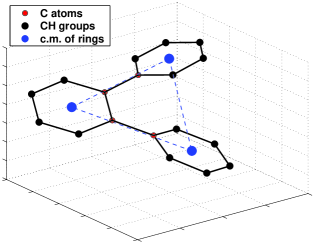
Figure 1: Color online: The structure of the ortho-terphenyl molecule (atomic coordinates from AMOS78 ).

The melting temperature of OTP is $T_{m}=330K$ and the boiling temperature is $T_{b}=605K$ BC27 . The “glass transition temperature” $T_{g}$ defined by volumetric and thermal measurements (cf. Figs. 3,5 below) is near $243K$ GT67 (This temperature depends on the thermal protocol by which the glass is prepared CB72 ).

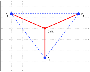
Figure 2: Color online: The planar LW-model of the ortho-terphenyl molecule.

II.2 The model employed in simulations

A simple coarse grained rigid model of OTP, known as the Lewis-Wahnström (L-W) model, was introduced for the first time in Refs. LW93 ; LW94 . Some intensive studies of the properties of this model were achieved by molecular dynamics (MD) simulations LW93 ; LW94 ; RST01 ; MNSDST02 ; CS04 ; LDS06 . More realistic representation of the OTP molecule consists in taking into account internal degrees of freedom and a number of models of such kind were developed and used in MD simulations KW95 ; MLRS00 ; MLRS01 ; GF06 ; BRDS06 .

For the sake of efficient numerical simulations the full resolution of the structure of the OTP molecule using a sufficiently large number of molecules is beyond our computer capabilities. One needs to invoke a reasonable model that can retain the essential aspects of the molecular structure while allowing reasonable computations. Therefore we choose the simple Lewis-Wahnström model and use it for Monte Carlo (MC) simulations. The OTP molecule is represented by a three-site complex, each site playing the role of the whole benzene ring (see Fig. 1). The interaction between two sites of different molecules is represented by a Lennard-Jones potential

$$\phi_{LJ}(r)=4\epsilon\Bigg{[}\bigg{(}\frac{\sigma}{r}\bigg{)}^{12}-\bigg{(}\frac{\sigma}{r}\bigg{)}^{6}\Bigg{]},$$ (1)

where $r$ is the distance between sites. For the sake of simulation speed we employ a smooth short range version of the interaction potential as proposed in MNSDST02

$$\phi(r)=\left\{\begin{array}[]{ll}\phi_{LJ}(r)+a+br&\textrm{if $r\leq r_{cut}$}\\ 0&\textrm{if $r>r_{cut}$}\end{array}\right.$$ (2)

Here, $\epsilon=5.276$ kJ/mol and $\sigma=0.483$ nm. The parameters $a$ and $b$ are chosen to guarantee the conditions $\phi(r_{cut})=0$ and the first derivative $\phi^{\prime}(r_{cut})=0$. For the cut-off distance $r_{cut}=1.2616$ nm the parameter values are $a=0.461$ kJ/mol, $b=-0.313$ kJ/(mol nm) MNSDST02 .

In the frame of the L-W model of OTP (see Fig. 2) the sites are placed at the vertices of a rigid isosceles triangle. The short sides of the triangle are of length $\sigma$ and the angle between them is $75^{o}$. The position of a site $\alpha$ ($\alpha=1,2,3$) in molecule $i$ is defined by

$$\vec{R}_{i,\alpha}=\vec{R}^{cm}_{i}+\vec{r}_{i,\alpha},$$ (3)

where $\vec{R}^{cm}_{i}$ denotes the position of the center of mass of molecule $i$. In the L-W model OTP molecules are treated as rigid bodies; each molecule has six (three rotations and three translations) degrees of freedom. Three of them are taken to be the Cartesian coordinates of the molecule center of mass (define the vector $\vec{R}^{cm}_{i}$) and other three are the Euler angles specifying the rotational position about the center of mass (defined by the vectors $\vec{r}_{i,\alpha}$).

The energy of interaction between two molecules is given by

$$U_{ij}=\sum\limits_{\alpha=1}^{3}\sum\limits_{\beta=1}^{3}\phi(\mid\vec{R}_{i,\alpha}-\vec{R}_{j,\beta}\mid).$$ (4)

II.3 Simulations details

We simulated $N=64$ and $N=512$ L-W OTP molecules in a cubic box with periodical boundary conditions in the frame of the Monte Carlo method MRRTT53 . The trial displacement of a molecule consists of usual random translation and random rotation (for details of rotations using Euler angles see OS77 ). The temperature dependence of the particle number density was estimated by simulations in an isothermal-isobaric (NPT) ensemble OS77 ; W68 with the pressure value fixed at $P=1$ bar. At each temperature the density was used in a canonical (NVT) ensemble Monte Carlo simulation. Having results in both ensembles enables us below to compare the specific heats at constant pressure and at constant volume to experiments. After short equilibration the average values of the quantities of interest in both ensembles were measured during $10^{7}$ sweeps in the case of a system with $N=64$ and $5\times 10^{6}$ for $N=512$ molecules. The acceptance rate was chosen to be $30\%$. A final configuration of MC simulations at constant pressure for $N=64$ particles in the simulation cell was used to create an initial configuration for simulation with the larger particle number $N=252$ (by using eight small cells to initiate one large cell). Final configurations of MC simulations at constant pressure were used as initial configurations for simulations at constant volume. The following dimensionless units are used: the dimensionless length is $r^{*}=r/\sigma$, the particle number density $\rho^{*}=\rho\sigma^{3}$, where $\rho=N/V$ ($V$ is the system volume), the temperature $T^{*}=k_{B}T/\epsilon$, where $k_{B}$ is the Boltzmann constant, the energy $U^{*}=U/\epsilon$, the pressure $P^{*}=P\sigma^{3}/\epsilon$ and the specific heat $C^{*}=C/(Nk_{B})$. In these dimensionless units $T_{m}^{*}=0.58$, $T_{b}^{*}=1.07$ and $T_{g}^{*}$ is near 0.43 .

II.4 Simulation results.

The temperature dependence of the particle number density at constant pressure is shown in Fig. 3.

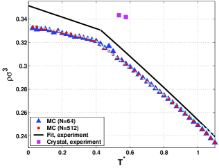
Figure 3: Color online: The particle number density as a function of the temperature from MC simulations at constant pressure. Blue triangles and red dots refer to $N=64$ and $N=512$ respectively. The solid black line shows the fit to the results of the experimental measurements for OTP (MFCR01 and references there). Experimental values for the crystal state of OTP ODCDES64 are shown for comparison as pink squares.

Obviously, we can not expect that the simple rigid molecular model of the OTP molecule should reproduce quantitatively the experimental data. Nevertheless, the qualitative behavior of the model is similar to the real system; the jump in the slope associated with the glass transition GT67 occurs at the temperature $T_{g}=0.4$, close to the experimental value. We have not studied the dependence of $T_{g}$ on the thermal protocol of the sample preparation in our simulations (see, e.g., PH99 ). The results of Fig. 3 are independent of the particle number in the simulation cell. This is an indication of negligible finite size effects.

Fig. 4 shows simulation results of the potential energy change with the temperature at the same conditions as Fig. 3.

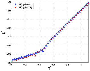
Figure 4: Color online: The potential energy of OTP model as a function of the temperature from MC simulations at constant volume.

The jump in the slope occurs at the same temperature $T_{g}=0.4$; again the data are not sensitive to the particle number in the simulation cell.

The specific heat at constant volume, $C_{v}$, and constant pressure, $C_{p}$, are defined by

$$\frac{C_{v}}{N} = \frac{\nu}{2}+\frac{\partial}{\partial T}\frac{\langle U\rangle}{N}\bigg{|}_{V}$$

$$= \frac{\nu}{2}+c_{v}$$

$$\frac{C_{p}}{N} = \frac{\nu}{2}+\frac{\partial}{\partial T}\frac{\langle U\rangle+PV}{N}\bigg{|}_{P}$$ (5)

$$= \frac{\nu}{2}+c_{p},$$

where $\nu$ is the number of degrees of freedom. The ’fluctuation’ part of the specific heat is defined at constant volume by

$$c_{v}=\frac{\langle{U^{*}}^{2}\rangle-\langle{U^{*}}\rangle^{2}}{N{T^{*}}^{2}},$$ (6)

where the potential energy $U^{*}$ is measured in the N-V-T ensemble and

$$c_{p}=\frac{\langle{H^{*}}^{2}\rangle-\langle{H^{*}}\rangle^{2}}{N{T^{*}}^{2}},$$ (7)

where $H^{*}=U^{*}-PV$ is measured in the N-P-T ensemble. Simulation results for OTP are displayed in Fig. 5.

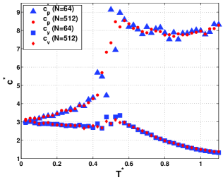
Figure 5: Color online: The temperature dependence of the specific heat in the OTP model at constant pressure and constant volume, such that the volume agrees with the constant pressure values (see Fig. 3).

Both specific heats show a drop near the temperature $T_{g}=0.4$ which is an indicator of the glass transition. In experiments one observes qualitative changes in $c_{p}$ as a function of the scanning speed T01 . Our simulations are qualitatively similar to what is observed in experiments with high scanning speed GT67 . With decreasing of the scanning speed the maximum of $c_{p}$ near the glass transition point disappears CB72 . We are not aware of experimental results on $c_{v}$ for low temperature OTP; however, similar behavior to ours near the glass transition point was observed in simulations of binary mixtures (see HIP08 ; HIPS08 ).

In order to look for possible structural peculiarities of OTP above $T_{g}$ we studied the radial pair distribution function of the molecular center of mass at different temperatures. Results for three temperatures are shown in Fig. 6. At high temperatures this function exhibits an ordinary structure typical to liquids with spherical particles. With decreasing the temperature the position of the first minimum is unchanged, however, the first peak displays a development of an internal structure with dips at low temperature. Similar behavior was detected in Molecular dynamics simulations LW94 . This can be attributed to the consequences of nonspherical intermolecular interactions; at low temperatures and high densities the system manifests local orientational ordering. Similar evolution of the pair distribution function was observed in simulations of hard spherocylinders and it was shown that at high packing fraction there exist short range orientational L94 .

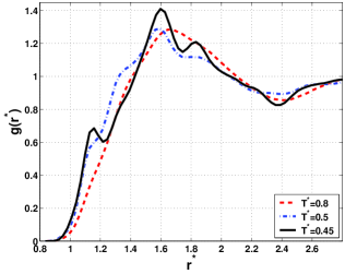
Figure 6: Color online: The radial pair distribution function of the OTP center of mass.

Finally we considered the coordination number defined for three dimensional systems as B77

$$\langle N\rangle=4\pi\rho\int\limits_{0}^{r_{min}}g(r)r^{2}\mathrm{d}r.$$ (8)

Here $r_{min}$ is the position of the first minimum of the pair distribution

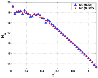
Figure 7: Color online: The temperature dependence of the coordination number.

function which is one of the possible measure of the range short order. The temperature dependence of the coordination number is important in thermodynamic models of the liquid state SRF80 . The position of $r_{min}$ is independent of temperature (see Fig. 6), therefore, another way to estimate the coordination number is to count the average number of neighbors inside the sphere of the radius $r_{min}$ (numerical result coincides with the direct integration in Eq. (8)). The result is displayed in Fig. 7. In the liquid state the temperature dependence is typical (see SRF80 ). In the vicinity of $T_{g}$ and below this value the slope is changed.

III Statistical Mechanics of the Glass Transition

III.1 Statistical geometry approach.

The structural properties of condensed matter can be investigated using scattering experiments (X-rays, electrons or neutrons scattering, see, e.g., Z79 ). The angular dependence of the scattering intensity is defined by the structure factor which is related to the pair distribution function. The scattering experiments on liquids and amorphous solids exhibit the presence of the short order in contrast to periodic crystals with long range order. If in a many-body system energy is presented only by two-body contributions the estimation of average thermodynamics values can be reduced to integrals involving the pair distribution function. Unfortunately, usually it is impossible to extract the pair distribution function from experimental data with the desired accuracy. This function is an average property and in the case of a multi-component systems even the interpretation of the structure of a system is difficult. Looking for example at Fig. 6 one sees that the radial pair distribution function is not a sufficiently revealing tool to allow a comprehensive discussion of the glass transition. As a replacement possible tool we turn now to the analysis of the structure of the super-cooled liquid in terms of local structures or quasi-species as defined below.

The first suggestion to characterize the state of liquids by local structures was offered by Bernal in B64 in the context of a model of hard balls. The idea is to invoke a geometrical approach to define the liquid structure. In contrast to a single component crystal with long-range order where all particles have the same number of neighbors, a liquid is random such that the number of neighbors is not fixed, and can vary quite significantly. Defining the concentration of central particles with $N$ nearest neighbors by $C_{N}$ with $N\in[N_{\rm min},N_{\rm max}]$, one understands that these concentrations will depend on the temperature and pressure, defining the ‘state’ of the liquid. This approach, which is referred to as ‘statistical geometry’, does not enjoy an exact method to calculate the distribution of concentrations $C_{N}$. On the other hand this distribution is readily obtained in computer simulations. In a series of papers (see for example BLPZ09 and references therein) it was shown that for glass formers made of point particles with soft interactions one can construct an approximate statistical mechanics that allows a reasonably accurate description of the evolution of the concentrations $C_{N}$ as a function of the temperature, with interesting implications for the study of the glass transition. In this paper we extend this approach to molecular liquids as explained below. The advantage of this approach (see for example F64 ) compared to say, approaches based on the pair distribution function, is that once the statistical mechanics is set up one can compute thermodynamic properties in the usual way that is found in any textbook on statistical physics.

III.2 Quasi-species in Supercooled Molecular Liquids

The crucial step in constructing an approximate theory is the identification of appropriate quasi-species. In the case of molecular liquids this task is not immediately obvious. As said above, we want to identify quasi-species which are made of a central molecule and a number of nearest neighbors, and these should have well defined configurations with well defined energies. The crucial assumption is that a given quasi-species interacts weakly with other quasi-species compared to the interaction of the central molecule with its nearest neighbors. As attractive as this this idea may sound, there are practical problems which appear if the number of such quasi-species required to describe the liquid configurations is not small. For example a non spherically symmetric molecule can take up many orientations relative to a given central molecule. Each orientation will result in a different energy of interaction. Take for example a situation in which the central molecule can have up to $N_{max}$ neighbors, and each neighbor molecule can be in two orientations. Then we already have $2^{N_{max}}$ possible configurations, each in principle having a different energy. Thus if $N_{max}=35$ we might have $\approx 3\times 10^{10}$ quasi-species–a ludicrous number that destroys the entire concept of quasi-species. To simplify things towards a workable theory (that will have to be validated against numerical data) we will treat all nearest neighbor sites as being identical, and the molecules occupying these sites as having $m$ internal degrees of freedom (for example orientations relative to the central molecule) with energies $\epsilon_{1},\dots,\epsilon_{m}$. The total energy of the quasi-species will be estimated as the sum of the energies of interaction of the neighbors with the central molecule. The interaction between the neighbors themselves will be estimated below as a ’crowding effect’ that will be characterized by a single additional parameter, following ideas prevalent in polymer physics. We turn now to a making these ideas concrete.

III.3 Statistical Mechanics of Quasi-species Concentrations

We begin by assuming that the neighboring molecules are not interacting with each other. In this case every neighboring molecule can have an energy taken from $m$ possible discrete values $\epsilon_{1},\cdots,\epsilon_{m}$. Denote by $N_{1}$ the number of ways that we can fit molecules with energy $\epsilon_{1}$, consistent with $N_{2}$ ways to fit molecules with energy $\epsilon_{2}$ etc. such that in total $N_{1}+N_{2}+\cdots+N_{m}=N$ where $N\leq N_{max}$ and $N_{max}$ is the maximum number of possible nearest neighbors. Then the number of such configurations is

$$\Omega(N_{1},\dots,N_{m}) = \frac{N_{max}!}{(N_{max}-N)!N!}\frac{N!}{\Pi_{k=1}^{m}N_{k}!}$$ (9)

$$= \frac{N_{max}!}{(N_{max}-N)!\Pi_{k=1}^{m}N_{k}!}.$$

As the energy of such a configuration is

$$U(N_{1},\dots,N_{m})=\sum_{k=1}^{m}N_{k}\epsilon_{k},$$ (10)

the Boltzmann weight of such a configuration is

$$W(N_{1},\dots,N_{m})=\Omega(N_{1},\dots,N_{m})e^{-\frac{\displaystyle{1}}{\displaystyle{k_{B}T}}\displaystyle{\sum_{k=1}^{m}N_{k}\epsilon_{k}}}$$ (11)

and consequently the total weight of any $N$ nearest neighbors is

$$W(N)=\sum_{N_{1}}\dots\sum_{N_{m}}W(N_{1},\dots,N_{m})\delta_{N,\sum_{k=1}^{m}N_{k}},$$ (12)

where $\delta_{i,j}$ is the Kronecker delta. Using the identity

$$\bigg{[}\sum_{k=1}^{m}e^{-\frac{\displaystyle{1}}{\displaystyle{k_{B}T}}\displaystyle{\epsilon_{k}}}\bigg{]}^{N}=\sum_{N_{1}}\dots\sum_{N_{m}}\frac{N!}{\Pi_{k=1}^{m}N_{k}!}$$ (13)

$$\times e^{-\frac{\displaystyle{1}}{\displaystyle{k_{B}T}}\displaystyle{\sum_{k=1}^{m}N_{k}\epsilon_{k}}}\delta_{N,\sum_{l=1}^{m}N_{l}}$$

Eq. (12) can be written explicitly as

$$W(N) = \sum_{N_{1}}\dots\sum_{N_{m}}\frac{N_{max}!}{(N_{max}-N)!\Pi_{k=1}^{m}N_{k}!}$$ (14)

$$\times e^{-\frac{\displaystyle{1}}{\displaystyle{k_{B}T}}\displaystyle{\sum_{k=1}^{m}N_{k}\epsilon_{k}}}\delta_{N,\sum_{l=1}^{m}N_{l}}$$

$$= \frac{N_{max}!}{(N_{max}-N)!N!}\bigg{[}\sum_{k=1}^{m}e^{-\frac{\displaystyle{1}}{\displaystyle{k_{B}T}}\displaystyle{\epsilon_{k}}}\bigg{]}^{N}.$$

Next we need to consider the interaction between neighboring molecules. Clearly, the assumption that the energy of a configuration is defined by Eq. (10) is correct only for $N\ll N_{max}$. The most obvious physical effect that destroys this assumption is the soft-core repulsive interaction that will exist between nearest neighbor molecule, especially as $N$ approaches $N_{max}$. To include such repulsive forces exactly is extremely cumbersome. In principle, if all nearest neighbor sites are not identical, the repulsive energies can vary between different pairs of nearest neighbor molecules. Even if these energies are identical the total repulsive energy will depend on the exact placement of $N$ nearest neighbor molecules in the available $N_{max}$ sites. Such considerations go beyond our desire to simplify the model as much as possible. We propose therefore a mean-field approximation in which the repulsive energy is described by only one new parameter. The reasoning is similar to that used in the polymer physics Z79 ; G79 . Suppose that there exists a soft core repulsive energy $J$ between each pair of nearest neighbor molecules in the first shell surrounding a central molecule. The probability that a nearest neighbor site is occupied is $N/N_{max}$ and therefore there will exist an additional term to the energy given by Eq. (10) due to this repulsive contribution,

$$U_{rep} = \frac{1}{2}J\frac{N}{N_{max}}N$$ (15)

$$= J\frac{N^{2}}{2N_{max}},$$

which is quadratic in $N$. Therefore, Eq. (14) is modified by the multiplication with the term $exp(-\frac{J}{k_{B}T}\frac{N^{2}}{2N_{max}})$ and the concentration of quasi particles with $N$ nearest neighbours reads

$$C_{N}=\frac{N_{max}!}{(N_{max}-N)!N!}\frac{\exp(\ln S(T)N-\frac{J}{k_{B}T}\frac{N^{2}}{2N_{max}})}{Z(T)},$$ (16)

where the partition function is

$$Z(T) = \sum_{N=1}^{N_{max}}\frac{N_{max}!}{(N_{max}-N)!N!}$$ (17)

$$\times \exp\bigg{(}\ln S(T)N-\frac{J}{k_{B}T}\frac{N^{2}}{2N_{max}}\bigg{)}$$

and

$$S(T)=\sum_{k=1}^{m}e^{-\frac{\displaystyle{\epsilon_{k}}}{\displaystyle{k_{B}T}}}.$$ (18)

III.4 Numerical results.

The most precise way to define ‘nearest neighbors’ is via the construction of a Voronoi tessellation (of polyhedra or polygons in three- or two- dimensional space correspondingly) V908 . In the frame of the Bernal approach this method was used in MC simulations to study the statistical geometry of the Lennard-Jones liquid FI70 ; FII70 .

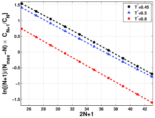
Figure 8: Color online: Chekup of Eq. 19 ($N_{max}=35$).

Unfortunately, the computational cost of a Voronoi construction is very high. A simpler definition of ‘nearest neighbors’ in MC or MD simulations was proposed in SNR83 . The nearest neighbors of a given particle are considered as particles with their centers inside the first coordination shell.

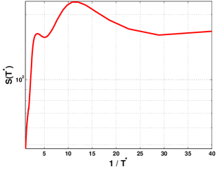
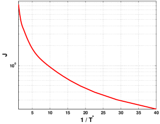
Figure 9: Color online: Upper panel: The function $S(T^{*})$ defined as the intercept in lines from Fig. 8. Lower panel: The parameter $J$defined as the slope in lines from Fig. 8 .

It was shown that if the second coordination shell is excluded the results are not sensitive to details of the nearest neighbors definition. Therefore, we counted a particle as a nearest neighbor of a central one if the distance between their centers of mass is less then $r_{min}$ in Eq. 8. The result of this calculation is given in terms of the temperature dependence of the concentration distribution $C_{N}$.

$$\ln{[\frac{(N+1)C_{N+1}}{(N_{max}-N)C_{N}}]}=\ln S(T)-\frac{J}{k_{B}T}\frac{2N+1}{2N_{max}}\ .$$ (19)

This suggests that if $\ln{[\frac{(N+1)C_{N+1}}{(N_{max}-N)C_{N}}]}$ is plotted against $2N+1$ there should result a straight line of slope $-\frac{J}{k_{B}T}\frac{1}{2N_{max}}$ and intercept $\ln S(T)$. Typical simulations results and comparison with the prediction of Eq. 19 are shown in Fig. 8. The slope and the intercept calculated by a least squares fit for different temperatures are plotted in Fig. 9.

From Eq. (18) the function $S(T)$ is given as a sum of exponentials. It turns out that it is very difficult to fit $S(T)$ as a sum of a small number of exponentials with temperature independent energies $\epsilon_{k}$. This may result from the fact that there are many such energies, or, as these are in fact phenomenological parameters, they are not at all guaranteed to be temperature independent, since they encapsulate information about the complicated interactions in the system. The same is true for the parameter $J$. Luckily, in the frame of the simple model proposed here we do not need the individual parameters $\epsilon_{k}$ since they always appear in the same combination in the form of the single function $S(T)$ (see Eq. 16). This function together with $J(T)$, both of which can be estimated from the simulations, are all that we need to determine the temperature dependence of the concentrations $C_{N}(T)$ which are the crucial observables in the present approach.

Having determined $S(T)$ and $J(T)$ from the numerics (cf. Fig. 9), the model prediction of the temperature dependence of $C_{N}(T)$ is shown in Fig, 10, in comparison with the direct numerical simulation results. The agreement appears excellent.

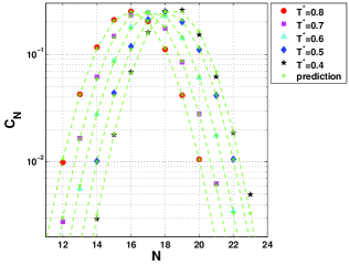
Figure 10: Color online: Temperature and $N$ dependence of $C_{N}(T)$. Symbols are the direct numerical simulations and dashed lines are correspond to the model prediction, Eq. 16 .

It is interesting to comment here that similar Gaussian looking distributions for a given temperature as a function of $N$ was found in all the models of glass formers that were studied using a similar quasi-species approach BLPZ09 . Close to the dependence displayed in Fig. 10 was observed in simulations of water model MSA11 . We believe that this is a generic feature that will be common to a very wide class of liquids and glass formers once the appropriate quasi-species are identified. The difference between one system and the other will be encoded in the temperature dependence of these Gaussian shapes. To see this we turn in Fig. 11 to a comparison of the direct numerical simulations to the model predictions for the temperature dependence of $C_{N}(T)$ at chosen values of $N$.

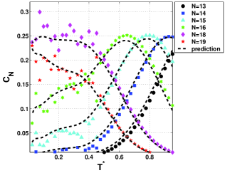
Figure 11: Color online: Dependence of the quasi-species concentration on the temperature at fix number of near neighbor particles. The dashed lines correspond to the model prediction Eq. 16 .

This may be the most relevant encoding of the subtle changes in the structure of the liquid as temperature is changed. We see (quite generically again) that some quasi-species decay in their concentration when temperature is decreased, some increase in concentration, and some first increase and then decrease to a finite value as $T\to 0$. The quasi-species whose concentration tends to zero are referred to here and in previous work as ‘liquid-like’, since their concentration is significant only in the high-temperature liquid. These are those associated with the highest free energy (made from both energy and degeneracy) and therefore their concentration declines when the temperature decreases. We will argue that they carry with them many of the signatures of the glass transition.

Like in previous studies ILLP07 it is worthwhile to group together all the quasi-species into three distinct groups according to their qualitative temperature dependence (decreasing, increasing, and first increasing and then decreasing). We refer to the resulting model as a ‘Doubly Coarse Grained’ (DCG) description. In the present case this means summing the following three groups

$$C_{I}\equiv\sum_{N=2}^{14}C_{N}(T)\ ,C_{II}\equiv\sum_{N=15}^{17}C_{N}(T)\ ,C_{III}\equiv\sum_{N=18}^{35}C_{N}(T)\ .$$ (20)

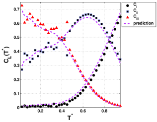
Figure 12: Color online: Comparison of MC simulations with the model prediction for grouped concentrations (see Eq. 20).

The temperature dependence of these three groups are shown in Fig. 12, again comparing the model predictions to the direct numerical simulation with an obvious excellent agreement. One can see that the glass transition temperature $T_{g}\sim 0.4$ corresponds to the intersection point of $C_{II}(T^{*})$ and $C_{III}(T^{*})$, at this point $C_{I}(T^{*})$ practically dies out.

The price of the ‘nearest neighbors’ definition used by us in contrast to the construction of a Voronoi tessellation is the loss of the information on a volume ascribed to a quasi-species. Nevertheless, one can try to use the definition of the perfect solution molar volume P57

$$v^{*}_{tot} = \sum\limits_{L=I}^{III}v^{*}_{L}(T^{*})$$ (21)

$$= \sum\limits_{L=I}^{III}\langle v^{*}\rangle_{L}C_{L}(T^{*}),$$

where $v^{*}_{tot}=1/\rho^{*}$. The partial volumes $\langle v^{*}\rangle_{L}$ were estimated by least squares fits in the whole temperature range and are displayed in Table 1.

Table 1: Color online: Partial volumes $\langle v^{*}\rangle_{L}$, densities $\rho^{*}_{L}$ and energies $\langle U^{*}\rangle_{L}$.

L	$\langle v^{*}\rangle_{L}$	$\rho^{*}_{L}$	$\langle U^{*}\rangle_{L}$
I	4.204	0.238	-9.13
II	3.651	0.298	-12.49
III	2.839	0.352	-17.29

The corresponding densities $\rho^{*}_{L}=1/\langle v^{*}\rangle_{L}$ are also presented in this table; one can see from the comparison with the data of Fig. 3 that the value of $\rho^{*}_{III}$ is close to the density of the crystal. Results for the temperature dependence of $v^{*}_{L}(T^{*})$ are shown in Fig. 13. The estimation of the molar volume by Eq. (21) is compared with MC data.

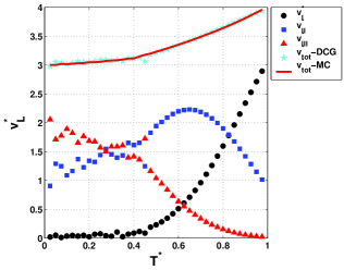
Figure 13: Color online: Volume contributions of the quasi-species.

In the frame of the approximation of the perfect solution the potential energy is given by

$$U^{*} = \sum\limits_{L=I}^{III}U^{*}_{L}(T^{*})$$ (22)

$$= \sum\limits_{L=I}^{III}\langle U^{*}\rangle_{L}C_{L}(T^{*}),$$

The coefficients $\langle U^{*}\rangle_{L}$ are estimated again by least squares fits in the whole temperature range and are displayed in Tab. 1. The contributions to the potential energy and the comparison of the potential energy from simulations and the prediction of Eq. (22) are shown in Fig. 14).

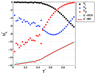
Figure 14: Color online: Energy contributions of the quasi-species.

The agreement of MC results and predictions of Eq. (21) and Eq. (22) means that in spite of the strong assumption of additivity in these equations the mixture of quasi-species can be effectively considered as a perfect solution.

The enthalpy can be connected with the quasi-species concentration using Eq. (21) and Eq. (22). Numerical differentiation of concentrations given by Eq. (20) yields the quasi-species contributions (see Eq. (5)). Results of these calculations and comparison with numerical differentiation of the enthalpy estimated in MC runs and data from Fig. 5 is displayed in Fig. 15. It follows from Fig. 13-Fig. 15 that the glass transition temperature defined by volumetric and thermal measurements can be associated with the disappearance of the quasi-species of kind $I$.

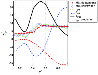
Figure 15: Color online: Contributions of the quasi-species to the heat capacity.

IV Local structures and viscosity of OTP

The theory of the viscosity of gases and liquids saw a long and confusing history, especially for super-cooled liquids, HCB54 ; B13 ; M23 ; H71 ; EZ72 ; A30 ; V21 ; F25 ; T25 ; TH26 ; MBCLSCS10 ; E36 ; AG65 ; RA98 ; G11 ; A05 ; HNOD08 ; SM09 ; A11 . For our purposes we refer to the interpolation formula that was proposed in D51 ; D57 ; CT59

$$\eta=\eta_{\infty}e^{A/v_{f}}.$$ (23)

Here $v_{f}$ is the free volume that in general is not easy to assign to any physical object. The idea behind this interpolation formula is that for particles to move out of their immediate cages some free volume needs to open up to allow flow. In our context it can be assumed that the decline in concentration of $C_{I}(T^{*})$ is responsible for the increase in viscosity; the free volume in this case is defined as $v^{*}_{f}=v^{*}_{I}(T^{*})$ (see also ABHIMPS07 ; HIMPS07 ). In order to confirm this suggestion it is necessary to consider the temperature dependence of the model free volume and the measured viscosity from the point of view of Eq. (23).

The temperature dependence of the dimensionless volume $v^{*}_{I}(T)$ shown in the upper panel of Fig. 17 above the glass transition temperature $T_{g}$ can be approximated by

$$\ln v^{*}_{I}(T)=3.3079-\frac{5.95T_{g}}{T}.$$ (24)

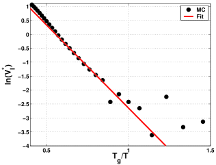
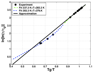
Figure 16: Color online: Upper panel: Temperature dependence of the volume $v^{*}_{I}(T)$. Lower panel:Temperature dependence of the experimental OTP viscosity PCC94 (the value of $\eta_{\infty}$ is taken from CE93 ).

The linearized temperature dependence of the measured OTP viscosity PCC94 is displayed in the lower panel of Fig. 16. In the vicinity of the glass transition temperature it is approximated by

$$\ln\ln\frac{\eta}{\eta_{\infty}}=-2.45+\frac{5.95T_{g}}{T},$$ (25)

where $\eta_{\infty}=1.25\times 10^{-3}$ poise is taken from CE93 for $T>283.3K$. Combination of Eq. (24) and Eq. (25) yields the free volume expression in the following form

$$\eta=\eta_{\infty}\exp{(v^{*}_{c}/v^{*}_{I}(T)})\ ,$$ (26)

where $v^{*}_{c}=2.36$.

In Fig, 17 we present the predictions of the last equation (26) to the experimental measurements of the viscosity in OTP as a function of $T/T_{g}$. The noise in our measurement of $C_{I}(T)$ and $v_{I}(T)$ (cf Figs. 12,13) is reflected in the scatter of the predicted viscosity. If we use the model prediction for $C_{I}(T)$ and $v_{I}(T)$ we find the solid red line.

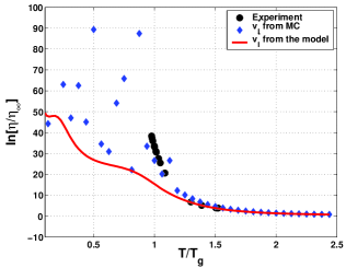
Figure 17: Color online: Comparison of the experimental measurements of the OTP viscosity PCC94 with the predictions of Eq. (26). Blue rhombi correspond to MC values of concentrations in Eq. (20), the solid red line represents calculation results with concentrations predicted by the model given by Eq. (16).

It follows from this figure that proposed definition of the free volume yields good agreement with the experimental data in the whole temperature range using the concentration as measured. The model prediction underestimates the viscosity at low temperatures; this must follow from a discrepancy between the model prediction and the actual simulational concentrations at these temperatures. Nevertheless, the simulation data indicates that below the glass transition temperature the rate of increase of the viscosity is slowing down. This conclusion agrees with the data in KTH00 .

V Discussion.

The basic assertion of this paper is that super-cooled liquids, be them simple or molecular liquids, are ergodic systems that are describable by statistical mechanics. It is quite impossible to write and to solve for the full partition function that takes into account all the interactions and the degrees of freedom in these systems. We have therefore developed a program in which we offer an approximate statistical mechanics that is based on considering, for every particle in the system, only the interactions with the nearest neighbors. This defines our ‘quasi-species’ which consist of a central particle and its $N$ neighbors, where $N$ can vary quite a bit. In many cases it turns out also advantageous to group the quasi-species into groups, such that one group consists of all the quasi-species whose concentrations decline when $T$ reduces. Usually another group contains all the quasi-species whose concentration increase as $T$ decreases, with a third group whose concentrations neither increases nor decreases BLPZ09 . We referred to the resulting model as the DCG model, in which the concentration of the first group acts as an order-parameter that signals the glass transition. In other words, since the quasi-species that disappear when $T\to 0$ are those of highest free energy, we consider them as them as liquid-like. In previous papers BLPZ09 we considered the inverse concentration of this group as a typical scale measuring the distance between the quasi-species raised to the appropriate power. Here we opted to compute numerically the volume associated with these disappearing objects and considered this as the ‘free volume’ of Eq. (23). Using this we could estimate the viscosity, and the results were compared to experiments in Fig. 17. It is quite gratifying to see the agreement between the predicted viscosity (blue rhombi) and the experimental data in the regime below the glass transition. We do not have data for $T<T_{g}$ from the experiment, but we still have (admittedly quite scattered) data for the functions $S(T)$ and $J(T)$ from which we can estimate the concentrations of the quasi-species. Using these we predict that the viscosity remains finite, even though extremely large (note the logarithmic scale in Fig. 17 ), even for $T\to 0$. We stress however that what really happens at $T=0$ cannot be safely deducted from the results of this study; it is much better to consider the theory of elasticity at $T=0$ as can be found in Ref. 11HKLP .

References

- (1) A. Cavagna, Supercooled liquids for pedestrians. Physics Reports 476, 51 (2009).
- (2) J-P. Eckmann and I. Procaccia, Ergodicity and slowing down in glass-forming systems with soft potentials: No finite-temperature singularities. Phys. Rev. E 78, 011503 (2008).
- (3) H.G.E. Hentschel, S. Karmakar, E. Lerner and I. Procaccia, Do athermal amorphous solids exist?”, Phys. Rev. E submitted. also: arXiv:1101.0101.
- (4) see for example L. Boué, E. Lerner, I. Procaccia, J. Zylberg, Predictive statistical mechanics for glass forming systems. J. Stat. Mech., P11010 (2009) and references therein.
- (5) D. Dhar and J. L. Lebowitz, Restricted equilibrium ensembles: Exact equation of state of a model glass. Euro. Phys. Lett. 92, 20008 (2010.
- (6) C.J.B.Clews, K. Lonsdale, Structure of 1.2-Diphenylbenzene (). Proc. R. Soc. Lond. A 161, 493-504 (1937).
- (7) I. L. Karle, L. O. Brockway, The structure of Biphenyl, o-Terphenyl and Tetraphenylene. J. Am. Chem. Soc. 66 1974-1979 (1944).
- (8) S. Aikawa, Y. Maruyama, Y. Ohashi, Y. Sasada, 1,2-Diphenylbenzene (o-Terphenyl). Acta Cryst. B34, 2901-2904 (1978).
- (9) G. M. Brown, H. A. Levy, o-Terphenyl by neutron diffraction. Acta Cryst. B35, 785-788 (1979).
- (10) W. E. Bachmann, H. T. Clarke, The mechanism of the wurtz-fitting reaction. J. Amer. Chem. Soc. 49, 2089-2098 (1927).
- (11) R. J. Greet, D. Turnbull, Glass transition in o-terphenyl. J. Chem. Phys. 46, 1243 (1967).
- (12) S. S. Chang, A. B. Bestul, Heat capacity and thermodynamic properties of o-terphenyl crystal, glass, and liquid. J. Chem. Phys. 56, 503-516 (1972).
- (13) L. J. Lewis, G. Wahnström, Relaxation of a molecular glass at intermediate times, Solid State Comm. 86, 295-299 (1993).
- (14) L. J. Lewis, G. Wahnström, Molecular-dynamics study of supercooled ortho-terphenil. Phys. Rev. B 50, 3865-3877 (1994).
- (15) A. Rinaldi, F. Sciortino, P. Tartaglia, Phys. Rev. E 63, 061210 (2001).
- (16) S. Mossa, E. La Nave, H. E. Stanley, C. Donati, F. Sciortino, P. Tartaglia, Dynamics and configurational entropy in the Lewis-Wahnström model for supercooled orthoterphenyl. Phys. Rev. E 65, 041205 (2002).
- (17) S. H. Chong, F. Sciortino, Structural relaxation in supercooled orthoterphenyl. Phys. Rev. E 69, 051202 (2004).
- (18) T. G. Lombardo, P. G. Debenedetti, F. H. Stillinger, Computational probes of molecular motion in the Lewis-Wahnström model for ortho-terphenyl. J. Chem. Phys. 125, 174507 (2006).
- (19) S. R. Kudchadkar, J. M. West, Molecular dynamics simulations of the glass former ortho-terphenyl. J. Chem. Phys. 103, 8566-8576 (1995).
- (20) S. Mossa, R. Di Leonardo, G. Ruocco, M. Sampoli, Molecular dynamics simulation of the fragile glass-former orthoterphenyl: A flexible molecule model. Phys. Rev. E 62, 612-639 (2000).
- (21) S. Mossa, R. Di Leonardo, G. Ruocco, M. Sampoli, Molecular dynamics simulation of the fragile glass-former orthoterphenyl: A flexible molecule model. II. Collective dynamics. Phys. Rev. E 64, 021511 (2001).
- (22) J. Ghosh, R. Faller, A comparative molecular simulation study of the glass former ortho-terphenyl in bulk and freestanding films. J. Chem. Phys. 125, 044506 (2006).
- (23) R. J. Berry, D. Rigby, D. Duan, M. Schwartz, Molecular dynamics study of translation and rotational diffusion in liquid ortho-terphenyl. J. Phys. Chem. A110, 13-19 (2006).
- (24) N. Metropolis, A. W. Rosenbluth, M. N. Rosenbluth, A. H. Teller, E. Teller,Equation of state calculations by fast computing machines. J. Chem. Phys. 21, 1087 (1953).
- (25) J. C. Owicki, H. A. Scheraga, Monte Carlo calculations in isothermal-isobaric ensemble. 1. liquid water. J. American Chem. Soc. 99, 7403-7412 (1977).
- (26) W. W. Wood, Monte Carlo Studies of Simple Liquid Models. In: H.N.V. Temperley, J.S. Rowlinson and G.S. Rushbrooke, Editors, The physics of simple liquids, North-Holland, Amsterdam, pp. 115-230 (1968).
- (27) G. Monaco, D. Fioretto, L. Comez, G. Ruocco, Glass transition and density fluctuations in the fragile glass former orthoterphenyl. Phys. Rev. E 63, 061502 (2001)
- (28) J. Opdycke, J. P. Dawson, R. K. Clark, M. Dutton, J. J. Ewing, H. H. Schmidt, Statistical thermodynamics of the polyphenyls. I. Molar volumes and compressibilities of biphenyl and m-, o-, and p-terphenyl. J. Phys. Chem. 68, 2385 (1954).
- (29) D. N. Pererra, P. Harrowell, Stability and structure of supercooled liquid mixture in two dimensions. Phys. Rev. E 59, 5721-5743 (1999).
- (30) A. Tölle, Neutron scattering studies of the model glass former ortho-terphenyl. Rep. Prog. Phys. 64, 1473-1532 (2001).
- (31) H. G. E. Hentschel, V. Ilyin, I. Procaccia, Nonuniversality of the specific heat in glass forming systems. Phys. Rev. Lett. 101, 265701 (2008).
- (32) H. G. E. Hentschel, V. Ilyin, I. Procaccia, N. Schupper, Theory of specific heat in glass-forming systems. Phys. Rev.E 78, 061504 (2008).
- (33) H. Löwen, Brownian dynamics of hard spherocylinders. Phys. Rev. E 50,1232-1242 (1994).
- (34) W. Brostow, Radial distribution function peaks and coordination numbers in liquids and amorphouse solids. Chem. Phys. Lett. 49, 285-288 (1977).
- (35) S. Skjold-Jørgensen, P. Rasmussen, A. Fredenslung, On the temperature dependence of the UNIQUAC/UNIFAC models. Chem. Eng, Sci. 35, 2389-2403 (1980).
- (36) J. M. Ziman, Models of disorder. The theoretical physics of homogeneously disordered systems. Cambridge University Press (1979).
- (37) J. D. Bernal, The structure of liquids. Proc. R. Soc. Lond. A280, 299-322 (1964).
- (38) R. Fürth, A new approach to the statistical thermodynamics of liquids. Proc. Roy. Soc. Edinb. A66, 232-251 (1963).
- (39) P. de Gennes, Scaling concepts in polymer physics. Cornell University Press (1979)
- (40) G. F. Voronoi, Nouvelles applications des paramètres continus à la théorie de formes quadratiques. J. reine angew. Math. 134, 198-287 (1908).
- (41) J. L. Finney, Random packing and the structure of simple liquids. I. The geometry of random close packing. Proc. R. Soc. Lond. A 319, 479-493 (1970).
- (42) J. L. Finney, Random packing and the structure of simple liquids. II. The molecular geometry of simple liquids. Proc. R. Soc. Lond. A 319, 495-507 (1970).
- (43) P. J. Steinhardt, D. R. Nelson, M. Ronchetti, Bond-orientational order in liquids and glasses. Phys. Rev. B 28, 784-805 (1983).
- (44) S. Merchant, J. K. Shah, D. Asthagiri, Water coordination structures and the excess free energy of liquids. arXiv:1101.1076v1 [physics.chem-ph] (2011).
- (45) V. Ilyin, E. Lerner, Ting-Shek Lo, I. Procaccia, Statistical mechanics of the glass transition in one-component liquids with an anisotropic potential. Phys. Rev. Lett. 99, 135702 (2007).
- (46) I. Prigogin, The molecular theory of solutions. avec A. Bellemans et V. Mathot; North-Holland Publ. Company, Amsterdam, 1957.
- (47) J. O. Hirschfelder, C. F. Curtiss, R. B. Bird, Molecular Theory of Gases and Liquids. John Wiley, New York (1954).
- (48) A. J. Batschinski, Untersuchungen über die innere Reibung der Flüessigkeiten, Z. Physik Chem. 84, 643-706 (1913)
- (49) D.B. Macleod , On a relation between the viscosity of a liquid and its coefficient of expansion. Trans. Farad. Soc. 19, 6-16 (1923).
- (50) J. H. Hildebrand,Motions of molecules in liquids: viscosity and diffusivity. Science 174, 490-493 (1971).
- (51) L. D. Eicher, B. J. Zwolinski, Limitations of the Hildebrand-Batschinski shear viscosity equation. Science 177, 369 (1972).
- (52) E. N. da C. Andrade, The Viscosity of Liquids, Nature 125, 309-310 (1930).
- (53) H. Vogel, Das Temperaturabhäungigkeitsgesetz der Viskosität von Flüssigkeiten. Phys. Zeit. 22, 645-646 (1921).
- (54) G. S. Fulcher, Analysis of recent measurements of the viscosity of glasses. J. Am. Ceram. Soc. 8, 339-355 (1925).
- (55) G. Tamman, Glasses as supercooled liquids. J. Soc. Glass Technol. 9, 166-185 (1925).
- (56) G. Tamman, W. Hesse, Die Abhängigkeit der Viscosität von der Temperatur bei unterkühlten Flüsigkeiten. Z. anorg. u. allgem. Chem. 156, 245-257 (1926).
- (57) H. Eyring, Viscosity, plasticity, and diffusion as examples of absolute reaction rates. J. Chem. Phys. 4, 283-291 (1936).
- (58) F. Mallamace, C. Branca, C. Corsaro, N. Leone, J. Spooren, S-H. Chen, H. E. Stanley, Transport properties of glass-forming liquids suggest that dynamic crossover temperature is an important as the glass transition temperature. PNAS 107, 22457-22462(2010).
- (59) G. Adam, J. H. Gibbs, On the temperature dependence of cooperative relaxation properties in glass-forming liquids. J. Chem Phys. 43, 139- (1965).
- (60) R. Richert, C. A. Angell, Dinamics of glass-forming liquids. Y. On the link between molecular dynamics and configurational entropy. J. Chem. Phys. 108, 9016-9026 (1998).
- (61) A. V. Granato, A derivation of the Vogel-Fulcher-Tamman relation for supercooled liquids. J. Non-cryst. Solids 357, 334-338 (2011).
- (62) I. Avramov, Viscosity in disordered media. J. Non-cryst. Solids 351, 3163-3173 (2005).
- (63) T. Hecksher, A. I. Nielsen, N. B. Olsen, J. C. Dyre, Little evidence for dynamic divergences in ultraviscous molecular liquidss. Nature Phys. 4, 737-741 (2008).
- (64) O. N. Senkov, D. B. Miracle, Descriprtion of the fragile behavior of glass-forming liquids with the use of experimentally accessible parameters. J. Non-cryst. Solids 355, 2596-2603 (2009).
- (65) I. Avramov, Interrelation between the parameters of equations of viscous flow and chemical composition of glassforming melts. J. Non-cryst. Solids 357, 391-396 (2011).
- (66) A. K. Doolittle, Studies in Newtonian flow. II. The dependence of the viscosity of liquids on free-space. J. Appl. Phys. 22, 1471-1475 (1951).
- (67) A. K. Doolittle, D. B. Doolittle, Studies in Newtonian flow. Y. Further verification of the free-space viscosity equation. J. Appl. Phys. 28, 901-905 (1957).
- (68) M. H. Cohen, D. Turnbull, Molecular transport in liquids and glasses. J. Chem. Phys. 31, 1164-1169 (1959).
- (69) E. Aharonov, E. Bouchbinder, H. G. E. Hentschel, V. Ilyin, N. Makedonska, I. Procaccia, N. Schupper, Direct identification of the glass transition: Growing length scale and the onset of plasticity. EPL 77, 56002 (2007).
- (70) H. G. E. Hentschel, V. Ilyin, N. Makedonska, I. Procaccia, N. Schupper, Statistical mechanics of the glass transition as revealed by a Voronoi tesselation. Phys. Rev. E 75, 050404(R) (2007).
- (71) D. J. Plazek, C. A. Beroa, I.-C. Chay, The recoverable compliance of amorphous materials. J. non-cryst. solids 172-174, 181-190 (1994).
- (72) M.T. Cicerone, M.D. Ediger, Photobleaching technique for measuring ultra-slow reorientation near and below the glass transition: the tetracene/o-terphenyl system. J. Phys. Chem. 97, 10489-10497 (1993).
- (73) H. Kobayashi, H. Takahashi, Y. Hiki, Viscosity of glasses near and below the glass transition temperature. J. Appl. Phys. 88, 3776-3778 (2000).