Multi-path Routing Metrics for
Reliable Wireless Mesh Routing Topologies

Abstract

Several emerging classes of applications that run over wireless networks have a need for mathematical models and tools to systematically characterize the reliability of the network. We propose two metrics for measuring the reliability of wireless mesh routing topologies, one for flooding and one for unicast routing. The Flooding Path Probability (FPP) metric measures the end-to-end packet delivery probability when each node broadcasts a packet after hearing from all its upstream neighbors. The Unicast Retransmission Flow (URF) metric measures the end-to-end packet delivery probability when a relay node retransmits a unicast packet on its outgoing links until it receives an acknowledgement or it tries all the links. Both metrics rely on specific packet forwarding models, rather than heuristics, to derive explicit expressions of the end-to-end packet delivery probability from individual link probabilities and the underlying connectivity graph.

We also propose a distributed, greedy algorithm that uses the URF metric to construct a reliable routing topology. This algorithm constructs a Directed Acyclic Graph (DAG) from a weighted, undirected connectivity graph, where each link is weighted by its success probability. The algorithm uses a vector of decreasing reliability thresholds to coordinate when nodes can join the routing topology. Simulations demonstrate that, on average, this algorithm constructs a more reliable topology than the usual minimum hop DAG.

I Introduction

Despite the lossy nature of wireless channels, applications that need reliable communications are migrating toward operation over wireless networks. Perhaps the best example of this is the recent push by the industrial automation community to move part of the control and sensing infrastructure of networked control systems (see [1] for a survey of the field) onto Wireless Sensor Networks (WSNs) [2, 3]. This has resulted in several efforts to create WSN communication standards tailored to industrial automation (e.g., WirelessHART [4], ISA-SP100 [5]).

A key network performance metric for all these communication standards is reliability, the probability that a packet is successfully delivered to its destination. The standards use several mechanisms to increase reliability via diversity, including retransmissions (time diversity), transmitting on different frequencies (frequency diversity), and multi-path routing (spatial / path diversity). But just providing mechanisms for higher reliability is not enough — methods to characterize the reliability of the network are also needed for optimizing the network and for providing some form of performance guarantee to the applications. More specifically, we need a network reliability metric in order to: 1) quickly evaluate and compare different routing topologies to help develop wireless node deployment / placement strategies; 2) serve as an abstraction / interface of the wireless network to the systems built on these networks (e.g., networked control systems); and 3) aid in the construction of a reliable routing topology.

This paper proposes two multi-path routing topology metrics, the Flooding Path Probability (FPP) metric and the Unicast Retransmission Flow (URF) metric, to characterize the reliability of wireless mesh hop-by-hop routing topologies. Both routing topology metrics are derived from the directed acyclic graph (DAG) representing the routing topology, the link probabilities (the link metric), and specific packet forwarding models. The URF and FPP metrics define different ways of combining link metrics than the usual method of summing or multiplying the link costs along single paths.

The merit of these routing topology metrics is that they clearly relate the modeling assumptions and the DAG to the reliability of the routing topology. As such, they help answer questions such as: When are interleaved paths with unicast hop-by-hop routing better than disjoint paths with unicast routing? Under what modeling assumptions does routing on an interleaved multi-path topology provide better reliability than routing along the best single path? What network routing topologies should use constrained flooding for good reliability? (These questions will be answered in Sections IV-D and V-D.)

Sections II and III provide background on routing topology metrics and a more detailed problem description, to better understand the contributions of this paper.

The contributions of this paper are two-fold: First, we define the FPP and URF metrics and algorithms for computing them in Sections IV and V. Second, we propose a distributed, greedy algorithm called URF-Delayed_Thresholds (URF-DT) to generate a mesh routing topology that locally optimizes the URF metric in Section VI. We demonstrate that the URF-DT algorithm can build routing topologies with significantly better reliability than the usual minimum hop DAG via simulations in Section VII.

II Related Works

In single-path routing, the path metric is often defined as the sum of the link metrics along the path. Examples of link metrics include the negative logarithm of the link probability (for path probability) [6], ETX (Expected Transmission Count), ETT (Expected Transmission Time), and RTT (Round Trip Time) [7]. Most single-path routing protocols find minimum cost paths, where the cost is the path metric, using a shortest path algorithm such as Dijkstra’s algorithm or the distributed Bellman-Ford algorithm [8].

In multi-path routing, one wants metrics to compare collections of paths or entire routing topologies with each other. Simply defining the multi-path metric to be the maximum or minimum single-path metric of all the paths between the source and the sink is not adequate, because such a multi-path metric will lose information about the collection of paths.

Our FPP metric is a generalization of the reliability calculations done in [9] for the M-MPR protocol and in [10] for the GRAdient Broadcast protocol. Unlike [9, 10], our algorithm for computing the FPP metric does not assume all paths have equal length.

Our URF metric is similar to the anypath route metric proposed by dubois-Ferriere et al. [6]. Anypath routing, or opportunistic routing, allows a packet to be relayed by one of several nodes which successfully receives a packet [11]. The anypath route metric generalizes the single-path metric by defining a “links metric” between a node and a set of candidate relay nodes. The specific “links metric” is defined by the candidate relay selection policy and the underlying link metric (e.g., ETX, negative log link probability). As explained later in Section V-D, although the packet forwarding models for the URF and FPP metrics are not for anypath routing, a variation of the URF metric is almost equivalent to the ERS-best E2E anypath route metric presented in [6].

One of our earlier papers, [12], modeled the precursor to the WirelessHART protocol, TSMP [13]. We developed a Markov chain model to obtain the probability of packet delivery over time from a given mesh routing topology and TDMA schedule. The inverse problem, trying to jointly construct a mesh routing topology and TDMA schedule to satisfy stringent reliability and latency constraints, is more difficult. The approach taken in this paper is to separate the scheduling problem from the routing problem, and focus on the latter. The works [14, 15] find the optimal schedule and packet forwarding policies for delay-constrained reliability when given a routing topology.

Many algorithms for building multi-path routing topologies try to minimize single-path metrics. For instance, [16] extends Dijkstra’s algorithm to find multiple equal-cost minimum cost paths while [17] finds multiple edge-disjoint and node-disjoint minimum cost paths. RPL [18], a routing protocol currently being developed by the IETF ROLL working group, constructs a DAG routing topology by building a minimum cost routing tree (links from child nodes to ”preferred parent” nodes) and then adding redundant links which do not introduce routing loops. In contrast, our URF-DT algorithm constructs a reliable routing topology by locally optimizing the URF metric, a multi-path metric that can express the reliability provided by hop-by-hop routing over interleaved paths.

Another difference between URF-DT and RPL is that URF-DT specifies a mechanism to control the order which nodes connect to the routing topology, while RPL does not. The connection order affects the structure of the routing topology.

Finally, the LCAR algorithm proposed in [6] for building a routing topology cannot be used to optimize the URF metric because the underlying link metric (negative log link probability) for the URF metric does not satisfy the physical cost criterion defined in [6].

III Problem Description

We focus on measuring the reliability of wireless mesh routing topologies for WSNs, where the wireless nodes have low computational capabilities, limited memory, and low-bandwidth links to neighbors.

Empirical studies [13] have shown that multi-path hop-by-hop routing is more reliable than single-path routing in wireless networks, where reliability is measured by the source-to-sink packet delivery ratio. The main problem is to define multi-path reliability metrics for flooding and for unicast routing that capture this empirical observation. The second problem is to design an algorithm to build a routing topology that directly tries to optimize the unicast multi-path metric.

The FPP and URF metrics only differ in their packet forwarding models, which are discussed in Sections IV-A and V-A. Both models do not retransmit packets on failed links. More accurately, a finite number of retransmissions on the same link can be treated as one link transmission with a higher success probability. Here, a failed link in the model describes a link outage that is longer than the period of the retransmissions (a bursty link).

In fact, without long link outages and finite retransmissions, it is hard to argue that multi-path hop-by-hop routing has better reliability than single-path routing. Under a network model where all the links are mutually independent and independent of their past state, all single paths have reliability 1 when we allow for an infinite number of retransmissions.

Both the FPP and URF metrics assume that the links in the network succeed and fail independently of each other. While this is not entirely true in a real network, it is more tractable than trying to model how links are dependent on each other. Both metrics also assume that each node can estimate the probability that an incoming or outgoing link fails through link estimation techniques at the link and physical layers [19].

III-A Notation and Terminology

We use the following notation and terminology to describe graphs. Let $G=({\mathcal{V}},{\mathcal{E}},p)$ represent a weighted directed graph with the set of vertices (nodes) ${\mathcal{V}}=\{1,\ldots,N\}$, the set of directed edges (links) ${\mathcal{E}}\subseteq\{(i,j)\>:\>i,j\in{\mathcal{V}}\}$, and a function assigning weights to edges $p:{\mathcal{E}}\mapsto[0,1]$. The edge weights are link success probabilities, and for more compact notation we use $p_{l}$ or $p_{ij}$ to denote the probability of link $l=(i,j)$. The number of edges in $G$ is denoted $E$. In a similar fashion to $G$, let $\bar{G}=(\bar{{\mathcal{V}}},\bar{{\mathcal{E}}},p)$ represent a weighted undirected graph (but now $\bar{{\mathcal{E}}}$ consists of undirected edges).

The source node is denoted $a$ and the sink (destination) node is denoted $b$. A vertex cut of $a$ and $b$ on a connected graph is a set of nodes ${\mathcal{C}}$ such that the subgraph induced by ${\mathcal{V}}\backslash{\mathcal{C}}$ does not have a single connected component that contains both $a$ and $b$. Note that this definition differs from the conventional definition of a vertex cut because $a$ and $b$ can be elements in ${\mathcal{C}}$.

The graph $G$ is a DODAG (Destination-Oriented DAG) if all the nodes in $G$ have at least one outgoing edge except for the destination node $b$, which has no outgoing edges. We say that a node $i$ is upstream of a node $j$ (and node $j$ is downstream of node $i$) if there exists a directed path from node $i$ to $j$ in $G$. Similarly, node $i$ is an upstream neighbor of node $j$ (and node $j$ is a downstream neighbor of node $i$) if $(i,j)$ is an edge in ${\mathcal{E}}$. The indegree of a node $i$, denoted as $\delta^{-}(i)$, is the number of incoming links, and similarly the outdegree of a node $i$, denoted as $\delta^{+}(i)$, is the number of outgoing links. The maximum indegree of a graph is $\Delta^{-}=\max_{i\in{\mathcal{V}}}\delta^{-}(i)$ and the maximum outdegree of a graph is $\Delta^{+}=\max_{i\in{\mathcal{V}}}\delta^{+}(i)$.

Finally, define $2^{\mathcal{X}}$ to be the set of all subsets of the set ${\mathcal{X}}$.

IV FPP Metric

This section presents the FPP metric, which assumes that multiple copies of a packet are flooded over the routing topology to try all possible paths to the destination.

IV-A FPP Packet Forwarding Model

In the FPP packet forwarding model, a node listens for a packet from all its upstream neighbors and multicasts the packet once on all its outgoing links once it receives a packet. There are no retransmissions on the outgoing links even if the node receives multiple copies of the packet. The primary difference between this forwarding model and general flooding is that the multicast must respect the orientation of the edges in the routing topology DAG.

IV-B Defining and Computing the Metric

• Flooding Path Probability Metric
  Let $G=({\mathcal{V}},{\mathcal{E}},p)$ be a weighted DODAG, where each link $(i,j)$ in the graph has a probability $p_{ij}$ of successfully delivering a packet and all links independently succeed or fail. The FPP metric $p_{a\rightarrow b}\in[0,1]$ for a source-destination pair $(a,b)$ is the probability that a packet sent from node $a$ over the routing topology $G$ reaches node $b$ under the FPP packet forwarding model. ∎

Since the FPP packet forwarding model tries to send copies of the packet down all directed paths in the network, $p_{a\rightarrow b}$ is the probability that a directed path of successful links exists in $G$ between the source $a$ and the sink $b$. This leads to a straightforward formula to calculate the FPP metric.

$$p_{a\rightarrow b}=\sum_{{\mathcal{E}}^{\prime}\in 2_{a\rightarrow b}^{\mathcal{E}}}\left(\prod_{l\in{\mathcal{E}}^{\prime}}p_{l}\prod_{\bar{l}\in{\mathcal{E}}\backslash{\mathcal{E}}^{\prime}}(1-p_{\bar{l}})\right)\qquad,$$ (1)

where $2_{a\rightarrow b}^{\mathcal{E}}$ is the set of all subsets of ${\mathcal{E}}$ that contain a path from $a$ to $b$. Unfortunately, this formula is computationally expensive because it takes $O(E2^{E})$ to compute.

Algorithm 1 computes the FPP metric $p_{a\rightarrow b}$ using dynamic programming and is significantly faster. The state used by the dynamic programming algorithm is the joint probability distribution of receiving a packet on vertex cuts ${\mathcal{C}}$ of the graph separating $a$ and $b$ (See Figure 1 for an example). Recall that our definition of ${\mathcal{C}}$ allows $a$ and $b$ to be elements of ${\mathcal{C}}$, which is necessary for the first and last steps of the algorithm.

Algorithm 1 Fast_FPP

Input: $G=({\mathcal{V}},{\mathcal{E}},p),a$ $\triangleright$ $G$ is a connected DAG.

Output: $\{p_{a\rightarrow v},\forall v\in{\mathcal{V}}\}$

${\mathcal{C}}:=\{a\}$ $\triangleright$ ${\mathcal{C}}$ is the vertex cut.

${\mathcal{V}}^{\prime}:={\mathcal{V}}\backslash a$ $\triangleright$ ${\mathcal{V}}^{\prime}$ is the set of remaining vertices.

5:${\mathcal{E}}^{\prime}:={\mathcal{E}}$ $\triangleright$ ${\mathcal{E}}^{\prime}$ is the set of remaining edges.

$u:=a$ $\triangleright$ $u$ is the node targeted for removal from ${\mathcal{C}}$.

$p_{\mathcal{C}}(\{a\}):=1$; $p_{\mathcal{C}}(\emptyset):=0$ $\triangleright$ pmf for vertex cut ${\mathcal{C}}$.

while ${\mathcal{V}}^{\prime}\neq\emptyset$ do

      [Find node $u$ to remove from vertex cut]

10:     if $u\not\in{\mathcal{C}}$ then

         Let ${\mathcal{J}}=\{j\,:\,\forall(i,j)\in{\mathcal{E}}^{\prime},i\in{\mathcal{C}}\}$

         $u:=\operatorname*{arg\,min}_{i\in{\mathcal{C}}}\big{|}\{(i,j)\in{\mathcal{E}}^{\prime}\,:\,j\in{\mathcal{J}}\}\big{|}$

     end if

      [Add node $v$ to vertex cut]

15:     Select any node $v\in\{j\in{\mathcal{V}}:(u,j)\in{\mathcal{E}}^{\prime}\}$

     $p_{\mathcal{C}}^{\prime}:=\mathtt{NIL}$ $\triangleright$ Probabilities for next vertex cut.

     for all subsets ${\mathcal{C}}^{\prime}$ of ${\mathcal{C}}$ do

         Let ${\mathcal{L}}=\{(i,v)\in{\mathcal{E}}^{\prime}\,:\,i\in{\mathcal{C}}^{\prime}\}$

         $p_{\mathcal{C}}^{\prime}({\mathcal{C}}^{\prime}\cup\{v\}):=p_{\mathcal{C}}({\mathcal{C}}^{\prime})\cdot\left(1-\prod_{l\in{\mathcal{L}}}(1-p_{l})\right)$

20:         $p_{\mathcal{C}}^{\prime}({\mathcal{C}}^{\prime}):=p_{\mathcal{C}}({\mathcal{C}}^{\prime})\cdot\prod_{l\in{\mathcal{L}}}(1-p_{l})$

     end for

     ${\mathcal{E}}^{\prime}:={\mathcal{E}}^{\prime}\backslash\{(i,v)\in{\mathcal{E}}^{\prime}\,:\,i\in{\mathcal{C}}\}$

     ${\mathcal{V}}^{\prime}:={\mathcal{V}}^{\prime}\backslash v$

     ${\mathcal{C}}:={\mathcal{C}}\cup\{v\}$

25:      [Compute path probability]

     Let $2_{v}^{\mathcal{C}}=\{{\mathcal{C}}^{\prime}\in 2^{\mathcal{C}}\,:\,v\in{\mathcal{C}}^{\prime}\}$

     $p_{a\rightarrow v}:=\sum_{{\mathcal{C}}^{\prime}_{v}\in 2_{v}^{\mathcal{C}}}p_{\mathcal{C}}^{\prime}({\mathcal{C}}^{\prime}_{v})$

      [Remove nodes ${\mathcal{D}}$ from vertex cut]

     Let ${\mathcal{D}}=\{i\in{\mathcal{C}}\,:\,\forall j,\,(i,j)\not\in{\mathcal{E}}^{\prime}\}$

30:     ${\mathcal{C}}:={\mathcal{C}}\backslash{\mathcal{D}}$

     $p_{\mathcal{C}}:=\mathtt{NIL}$

     for all subsets ${\mathcal{C}}^{\prime}$ of ${\mathcal{C}}$ do

         $p_{\mathcal{C}}({\mathcal{C}}^{\prime}):=\sum_{{\mathcal{D}}^{\prime}\in 2^{\mathcal{D}}}p_{\mathcal{C}}^{\prime}({\mathcal{C}}^{\prime}\cup{\mathcal{D}}^{\prime})$

     end for

35:end while

Return: $\{p_{a\rightarrow v},\forall v\in{\mathcal{V}}\}$

Figure 1: An example of a sequence of vertex cuts that can be used by Algorithm 1. The vertex cut after adding and removing nodes from each iteration of the outer loop is circled in red.

Figure 2: Running Algorithm 1 on the network graph shown on the left when selecting vertex cuts in the order depicted in Figure 1 is equivalent to creating the vertex cut DAG shown on the right and finding the probability that state $a$ will transition to state $b$.

Conceptually, the algorithm is converting the DAG representing the network to a vertex cut DAG, where each vertex cut at step $k$, ${\mathcal{C}}^{(k)}$, is represented by the set of nodes ${\mathcal{S}}^{(k)}=2^{{\mathcal{C}}^{(k)}}$. Each node in ${\mathcal{S}}^{(k)}$ represents the event that a particular subset of the vertex cut received a copy of the packet. The algorithm computes a probability for each node in ${\mathcal{S}}^{(k)}$, and the collection of probabilities of all the nodes in ${\mathcal{S}}^{(k)}$ represent the joint probability distribution that nodes in the vertex cut ${\mathcal{C}}^{(k)}$ can receive a copy of the packet. A link in the vertex cut DAG represents a valid (nonzero probability) transition from a subset of nodes that have received a copy of the packet in ${\mathcal{C}}^{(k-1)}$ to a subset of nodes that have received a copy of the packet in ${\mathcal{C}}^{(k)}$. Figure 2 shows an example of this graph conversion using the selection of vertex cuts depicted in Figure 1.

Algorithm 1 tries to keep the vertex cut small by using the greedy criteria in lines 10–15 to adds nodes to the vertex cut. A node can only be added to the vertex cut if all its incoming links originate from the vertex cut. When a node is added to the vertex cut, its incoming links are removed. A node is removed from the vertex cut if all its outgoing links have been removed.

Computing the path probability $p_{a\rightarrow b}$ reduces to computing the joint probability distribution that a packet is received by a subset of the vertex cut in each step of the algorithm. The joint probability distribution over the vertex cut ${\mathcal{C}}^{(k)}$ is represented by the function $p_{\mathcal{C}}^{(k)}:{\mathcal{S}}^{(k)}\mapsto[0,1]$. Step $k$ of the algorithm computes $p_{\mathcal{C}}^{(k)}$ from $p_{\mathcal{C}}^{(k-1)}$ on lines 19, 20, and 33 in Algorithm 1. Notice that the nodes in each ${\mathcal{S}}^{(k)}$ represent disjoint events, which is why we can combine probabilities in lines 27 and 33 using summation.

IV-C Computational Complexity

The running time of Algorithm 1 is $O\big{(}N(\hat{C}\Delta^{+}+2^{\hat{C}}\Delta^{-})\big{)}$, where $\hat{C}$ is the size of the largest vertex cut used in the algorithm. This is typically much smaller than the time to compute the FPP metric from (1), especially if we restrict flooding to a subgraph of the routing topology with a small vertex cut. The analysis to get the running time of Algorithm 1 can be found in Section 2.2.2 of the dissertation [20].

The main drawback with the FPP metric is that it cannot be computed in-network with a single round of local communication (i.e., between 1-hop neighbors). Algorithm 1 requires knowledge of the outgoing link probabilities of a vertex cut of the network, but the nodes in a vertex cut may not be in communication range of each other. Nonetheless, if a gateway node can gather all the link probabilities from the network, it can give an estimate of the end-to-end packet delivery probability (the FPP metric) to systems built on this network.

IV-D Discussion

Figure 3 shows the probability of nodes in a mesh network receiving a packet flooded from the source. This simple topology shows that a network does not need to have large vertex cuts to have good reliability in a network with poor links. In regions of poor connectivity, flooding constrained to a directed acyclic subgraph with a small vertex cut can significantly boost reliability.

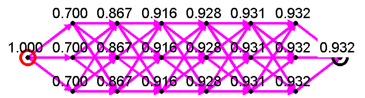
Figure 3: FPP metric $p_{a\rightarrow v}$ for all nodes $v$, where all links have probability $0.7$. The source node $a$ is circled in red.

Oftentimes, it is not possible to estimate the probability of the links accurately in a network. Fortunately, since the FPP metric is monotonically increasing with respect to all the link probabilities, the range of the FPP metric can be computed given the range of each link probability. The upper (lower) bound on $p_{a\rightarrow b}$ can be computed by replacing every link probability $p_{l}$ with its respective upper (lower) bound $\overline{p}_{l}$ ($\underline{p}_{l}$) and running Algorithm 1. For instance, the FPP metrics in Figure 3 can be interpreted as a lower bound on the reliability between the source and each node if all links have probability greater than $0.7$.

V URF Metric

This section presents the URF metric, which assumes that a single copy of the packet is routed hop-by-hop over the routing topology. Packets are forwarded without prior knowledge of which downstream links have failed.

V-A URF Packet Forwarding Model

Under the URF packet forwarding model, a node that receives a packet will select a link uniformly at random from all its outgoing links for transmission. If the transmission fails, the node will select another link for transmission uniformly at random from all its outgoing links that have not been selected for transmission before. This repeats until either a transmission on a link succeeds or the node has attempted to transmit on all its outgoing links and failed each time. In the latter case, the packet is dropped from the network.

V-B Defining and Computing the Metric

• Unicast Retransmission Flow Metric
  Let $G=({\mathcal{V}},{\mathcal{E}},p)$ be a weighted DODAG, where each link $(i,j)$ in the graph has a probability $p_{ij}$ of successfully delivering a packet and all links independently succeed or fail. The URF metric $\varrho_{a\rightarrow b}\in[0,1]$ for a source-destination pair $(a,b)$ is the probability that a packet sent from node $a$ over the routing topology $G$ reaches node $b$ under the URF packet forwarding model. ∎

The URF metric $\varrho_{a\rightarrow b}$ can be computed using

$$\varrho_{a\rightarrow a} =1$$ (2)

$$\varrho_{a\rightarrow v} =\sum_{u\in{\mathcal{U}}_{v}}\varrho_{a\rightarrow u}\varpi_{uv}\qquad,$$

where ${\mathcal{U}}_{v}$ are all the upstream neighbors of node $v$ and $\varpi_{uv}\in[0,1]$ is the Unicast Retransmission Flow weight (URF weight) of link $(u,v)$. The URF weight for link $l=(u,v)$ is the probability that a packet at $u$ will traverse the link to $v$, and is given by

$$\varpi_{uv}=\sum_{{\mathcal{E}}^{\prime}\in 2^{{\mathcal{E}}_{u}\backslash l}}\frac{p_{uv}}{|{\mathcal{E}}^{\prime}|+1}\left(\prod_{e\in{\mathcal{E}}^{\prime}}p_{e}\right)\left(\prod_{\bar{e}\in{\mathcal{E}}_{u}\backslash({\mathcal{E}}^{\prime}\cup l)}1-p_{\bar{e}}\right)$$ (3)

where ${\mathcal{E}}_{u}=\{(u,v)\in{\mathcal{E}}:v\in{\mathcal{V}}\}$ is the set of node $u$’s outgoing links.

Next, we sketch how (2) and (3) can be derived from the URF packet forwarding model. Recall that only one copy of the packet is sent through the network and the routing topology is a DAG, so the event that the packet traverses link $(u_{1},v)$ is disjoint from the event that the packet traverses $(u_{2},v)$. The probability that a packet sent from $a$ traverses link $(u,v)$ is simply $\varrho_{a\rightarrow u}\varpi_{uv}$, where $\varrho_{a\rightarrow u}$ is the probability that a packet sent from node $a$ visits node $u$ (therefore, $\varrho_{a\rightarrow a}=1$). Thus, the probability that the packet visits node $v$ is the sum of the probabilities of the events where the packet traverses an incoming edge of node $v$, as stated in (2).

Now, it remains to show that $\varpi_{uv}$ as defined by (3) is the probability that a packet at $u$ will traverse the link $(u,v)$. Recall that a packet at $u$ will traverse $(u,v)$ if all the previous links selected by $u$ for transmission fail and link $(u,v)$ is successful. Alternately, this event can be described as the union of several disjoint events arising from two independent processes:

• each of $u$’s outgoing links is either up or down (with its respective probability), and

• $u$ selects a link transmission order uniformly at random from all possible permutations of its outgoing links.

Each disjoint event is the intersection of: a particular realization of the success and failure of $u$’s outgoing links where $(u,v)$ is successful (corresponding to $p_{uv}\prod p_{e}\prod(1-p_{\bar{e}})$ in (3)); and a permutation of the outgoing links where $(u,v)$ is ordered before all the other successful links (corresponding to $1/(|{\mathcal{E}}^{\prime}|+1)$ in (3)). Summing the probabilities of these disjoint events yields (3). For a rigorous derivation of the URF weights from the packet forwarding model, please see Section 2.3.3 of the dissertation [20].

V-C Computational Complexity

The slowest step in computing the URF metric between all nodes and the sink is computing (3), which has complexity $O(\Delta^{+}\cdot 2^{\Delta^{+}})$. Using some algebra (See the Appendix), (3) simplifies to

$$\varpi_{uv}=p_{uv}\int_{0}^{1}\prod_{e\in{\mathcal{E}}_{u}\backslash(u,v)}\left(1-p_{e}x\right)dx\qquad,$$ (4)

which can be evaluated efficiently in $O((\Delta^{+})^{2})$. This results from the $O((\Delta^{+})^{2})$ operations to expand the polynomial and $O(\Delta^{+})$ operations to evaluate the integral. Since there are $O(\Delta^{+})$ link weights per node and $N$ nodes in the graph, the complexity to compute the URF metric sequentially on all nodes in the graph is $O(N(\Delta^{+})^{3})$. (There are also $O(E)$ operations in (2), but $E<2N\Delta^{+}$.) If we allow the link weights to be computed in parallel on the nodes, then the complexity becomes $O((\Delta^{+})^{3}+E)$.

Unlike the FPP metric, The URF metric can be computed in-network with local message exchanges between nodes. First, each node would locally compute the URF link weights $\varpi_{uv}$ from link probability estimates on its outgoing links. Then, since the URF metric $\varrho_{a\rightarrow v}$ is a linear function of the URF weights, we can rewrite (2) as

$$\varrho_{b\rightarrow b} =1$$ (5)

$$\varrho_{u\rightarrow b} =\sum_{v\in{\mathcal{V}}_{u}}\varpi_{uv}\varrho_{v\rightarrow b}\qquad,$$

where ${\mathcal{V}}_{u}$ are all the downstream neighbors of node $u$. This means that each node $u$ only needs the URF metric of its downstream neighbors to compute its URF metric to the sink, so the calculations propagate outwards from the sink with only one message exchange on each link in the DAG.

V-D Discussion

The URF forwarding model can be implemented in both CSMA and TDMA networks. In the latter it describes a randomized schedule that is agnostic to the quality of the links and routes in the network, such that the scheduling problem is less coupled to the routing problem. Loosely speaking, such a randomized packet forwarding policy is also good for load balancing and exploiting the path diversity of mesh networks.

The definition of the URF link weights is tightly tied to the URF packet forwarding model. One alternate packet forwarding model would be for a node to always attempt transmission on outgoing links $(u,v)$ in decreasing order of downstream neighbor URF metrics $\varrho_{v\rightarrow b}$. As before, the node tries each link once and drops the packet when all links fail. This model leads to the following Remaining-Reliability-ordered URF metric (RRURF), $\varrho_{a\rightarrow b}^{\prime}$, also calculated like $\varrho_{a\rightarrow b}$ from (5) except $\varpi_{uv}$ is replaced by

$$\varpi_{l_{i}}^{\prime}=\prod_{k=1}^{i-1}(1-p_{l_{k}})p_{l_{i}}\quad,$$ (6)

where the outgoing links of node $u$ have been sorted into the list $(l_{1},\ldots,l_{\delta^{+}(u)})$ from highest to lowest downstream neighbor URF metrics.

Notice that with unicast, a packet can reach a node where all its outgoing links fail, i.e., the packet is “trapped at a node.” Thus, topologies where a node is likely to receive a packet but has outgoing links with very low success probabilities tend to perform poorly. Flooding is not affected by this phenomenon of “trapped packets” because other copies of the packet can still propagate down other paths. In fact, given the same routing topology $G$, the URF metric $\varrho_{a\rightarrow v}$ is always less than the FPP metric $p_{a\rightarrow v}$ for all nodes $v$ in the network. The URF and FPP metrics allow us to compare how much reliability is lost when unicasting packets. A comparison of Figure 4 with Figure 3 reveals that this drop in reliability can be significant in deep networks with low probability links. Nonetheless, unicast routing over a mesh still provides much better reliability than routing down a single path or a small number of disjoint paths with the same number of hops and the same link probabilities, if the links are independent and bursty.

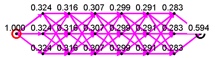
Figure 4: URF metric $\varrho_{a\rightarrow v}$ for all nodes $v$, where all links have probability $0.7$. The source node $a$ is circled in red.

Below are several properties of the URF metric that will be exploited in Section VI to build a good mesh routing topology.

Property 1 (Trapped Packets)

Adding an outgoing link to a node can lower its URF metric. Similarly, increasing the probability of an outgoing link can also lower a node’s URF metric. ∎

Property 1 can be seen on the example shown in Figure 5a. Here, link $(2,1)$ lowers the reliability of node $2$ to $b$. Generally, nodes want to route to other nodes that have better reliability to the sink, but Figure 5b shows an example where routing to a node with worse reliability can increase your reliability.

(a) Illustration of Property 1.

(b) Illustration of Property 2.

Figure 5: Links are labeled with probabilities, and nodes are labeled with URF metrics $\varrho_{v\rightarrow b}$ (boxed). LABEL:sub@fig:urf_3_node_example1 Increasing $p_{12}$ lowers node 2’s reliability. LABEL:sub@fig:urf_3_node_example2 Node 1 has a lower probability link to the sink than node 2, but link $(2,1)$ boosts the reliability of node 2.

Property 2

A node $u$ may add an outgoing link to node $v$, where $\varrho_{v\rightarrow b}<\varrho_{u\rightarrow b}$, to increase $u$’s URF metric. ∎

Property 2 means that adding links between nodes with poor reliability to the sink can boost their reliability, as shown in Figure 6.

Figure 6: Nodes can significantly increase their reliabilities using cross links. Links are labeled with probabilities, and nodes are labeled with URF metrics $\varrho_{v\rightarrow b}$ (boxed). Without the cross links (the links with probability 1 in the diagram), the nodes would all have URF metric $0.5$.

Property 3

Increasing the URF metric of a downstream neighbor of node $u$ always increases $u$’s URF metric. ∎

Property 3 is because $\varrho_{u\rightarrow b}$, defined by (2), is monotonically increasing in $\varrho_{v\rightarrow b}$ for all $v$ that are downstream neighbors of $u$.

Property 4

A node may have a greater URF metric than some of its downstream neighbors (from Property 2), but not a greater URF metric than all of its downstream neighbors. ∎

Property 4 comes from

$$\varrho_{u\rightarrow b}=\sum_{v\in{\mathcal{V}}_{u}}\varpi_{uv}\varrho_{v\rightarrow b}\leq(\max_{v\in{\mathcal{V}}_{u}}\varrho_{v\rightarrow b})\sum_{v\in{\mathcal{V}}_{u}}\varpi_{uv}\leq\max_{v\in{\mathcal{V}}_{u}}\varrho_{v\rightarrow b}.$$

Not surprisingly, Properties 3 and 4 highlight the importance of ensuring that nodes near the sink have a very high URF metric $\varrho_{v\rightarrow b}$ when deploying networks and building routing topologies.

If there is uncertainty estimating the link probabilities, bounding the URF metric is not as simple as bounding the FPP metric because the URF metric is not monotonically increasing in the link probabilities, as noted in Property 1. However, the URF metric $\varrho_{u\rightarrow b}$ is monotonically increasing with the link flow weights $\varpi_{uv}$ so bounds on the flow weights can be used to compute bounds on the URF metric by simple substitution. Similarly, each flow weight varies monotonically with each link probability, so it can also be bounded by simple substitution. For instance, to compute the upper bound of $\varpi_{uv}$, you would substitute the upper bound $\overline{p_{uv}}$ for $p_{uv}$ and the lower bounds $\underline{p_{e}}$ for all the other links in (4). Note that the upper bounds for all the flow weights on the outgoing links from a node may sum to a value greater than 1, which would lead to poor bounds on the URF metric.

VI Constructing a Reliable Routing Topology

The URF-Delayed_Thresholds (URF-DT) algorithm presented below uses the URF metric to help construct a reliable, loop-free routing topology from an ad-hoc deployment of wireless nodes. The algorithm assumes that each node can estimate the packet delivery probability of its links. Only symmetric links, links where the probability to send and receive a packet are the same, are used by the algorithm. The algorithm either removes or assigns an orientation to each undirected link in the underlying network connectivity graph to indicate the paths a packet can follow from its source to its destination. The resulting directed graph is the routing topology.

To ensure that the routing topology is loop-free, the URF-DT algorithm assigns an ordering to the nodes and only allows directed edges from larger nodes to smaller nodes. The algorithm assigns a mesh hop count to each node to place them in an ordering, analogous to the use of rank in RPL [18].

The URF-DT algorithm is distributed on the nodes in the network and constructs the routing topology (a DODAG) outward from the destination. Each node uses the URF metric to decide how to join the network — who it should select as its downstream neighbors such that packets from the node are likely to reach the sink. A node has an incentive to join the routing topology after its neighbors have joined, so they can serve as its downstream neighbors and provide more paths to the sink. To break the stalemate where each node is waiting for another node to join, URF-DT forces a node to join the routing topology if its reliability to the sink after joining would cross a threshold. This threshold drops over time to allow all nodes to eventually join the network.

VI-A URF Delayed Thresholds Algorithm

The URF-DT algorithm given in Algorithm 2 operates in rounds, where each round lasts a fixed interval of time. The algorithm requires all the nodes share a global time (e.g., by a broadcast time synchronization algorithm) so they can keep track of the current round $k$.

Algorithm 2 URF-Delayed_Thresholds

Input: connectivity graph $\bar{G}=(\bar{{\mathcal{V}}},\bar{{\mathcal{E}}},p),b,\bm{\tau},K$

Output: routing topology $G=({\mathcal{V}},{\mathcal{E}},p)$, mesh hop counts $\bm{\hbar}$

${\mathcal{V}}:=\emptyset,{\mathcal{E}}:=\emptyset$

$\forall i,\hbar_{i}:=\mathtt{NIL}$ $\triangleright$ $\mathtt{NIL}$ means not yet assigned.

$\hbar_{b}:=0$

for $k:=1$ to $K$ do

      [Run this code simultaneously on all nodes $u\not\in{\mathcal{V}}$]

     Let $\hbar_{{\mathcal{V}}_{u}}^{\mathrm{min}}=\min_{v\in{\mathcal{V}}_{u}}\hbar_{v}\;,\;\hbar_{{\mathcal{V}}_{u}}^{\mathrm{max}}=\max_{v\in{\mathcal{V}}_{u}}\hbar_{v}$

     for $h:=\hbar_{{\mathcal{V}}_{u}}^{\mathrm{min}}+1$ to $\hbar_{{\mathcal{V}}_{u}}^{\mathrm{max}}+1$ do

          ${\mathcal{V}}_{u}^{<h}$ are $u$’s neighbors with hop count less than $h$.

         Select ${\mathcal{V}}_{u}^{\star}\subseteq{\mathcal{V}}_{u}^{<h}$ to maximize $\varrho_{u\rightarrow b}$ from (4), (5).

         Let $\varrho_{u\rightarrow b}^{\star}$ be the maximum $\varrho_{u\rightarrow b}$.

         if $\varrho_{u\rightarrow b}^{\star}\geq\tau_{k-h+1}$ then

              $\hbar_{u}:=h$

              Add $u$ to ${\mathcal{V}}$. Add links $\{(u,v):v\in{\mathcal{V}}_{u}^{\star}\}$ to ${\mathcal{E}}$.

              Break from for loop over $h$.

         end if

     end for

end for

Return: $G,\bm{\hbar}$

At each round $k$, a node $u$ decides whether it should join the routing topology with mesh hop count $\hbar_{u}$. If node $u$ joins with hop count $\hbar_{u}$, then $u$’s downstream neighbors are the neighbors $v_{i}$ with a mesh hop count less than $\hbar_{u}$ that maximize $\varrho_{u\rightarrow b}$ from (5). Node $u$ decides whether to join the topology, and with what mesh hop count $\hbar_{u}$, by comparing the maximum reliability $\varrho_{u\rightarrow b}^{\star}$ for each mesh hop count $h\in\{\min_{v\in{\mathcal{V}}_{u}}\hbar_{v}+1,\ldots,\max_{v\in{\mathcal{V}}_{u}}\hbar_{v}+1\}$ with a threshold $\tau_{m}$ that depends on $h$. The threshold $\tau_{m}$ is selected from a predefined vector of thresholds $\bm{\tau}=[\tau_{1}\;\cdots\;\tau_{M}]\in[0,1]^{M}$ using the index $m=k-h+1$, as shown in Figure 7. When there are multiple $h$ with $\varrho_{u\rightarrow b}^{\star}\geq\tau_{m}$, node $u$ sets its mesh hop count $\hbar_{u}$ to the smallest $h$. If none of the $h$ have $\varrho_{u\rightarrow b}^{\star}\geq\tau_{m}$, then node $u$ does not join the network in round $k$.

Figure 7: Illustration of how thresholds are used to help assign a node a mesh hop count. The horizontal row of thresholds represent $\bm{\tau}$. The shaded vertical column of thresholds are the thresholds tested by a node in round $k$. A node $u$ picks the smallest mesh hop count $h$ such that $\varrho_{u\rightarrow b}^{\star}\geq\tau_{m}$ (see text for details).

For the algorithm to work correctly, the thresholds $\bm{\tau}$ must decrease with increasing $m$. The network designer gets to choose $\bm{\tau}$ and the number of rounds $K$ to run the algorithm. URF-DT can construct a better routing topology if $\bm{\tau}$ has many thresholds that slowly decrease with $m$, but the algorithm will take more rounds to construct the topology.

Algorithm 2 is meant to be implemented in parallel on the nodes in the network. All the nodes have the vector of thresholds $\bm{\tau}$. In each round, each node $u$ listens for a broadcast of the pair $(\varrho_{v_{i}\rightarrow b}$, $\hbar_{v_{i}})$ from each of its neighbors $v_{i}$ that have joined the routing topology. After receiving the broadcasts, node $u$ performs the computations and comparisons with the thresholds to determine if it should join the routing topology with some mesh hop count $\hbar_{u}$. Once $u$ joins the network, it broadcasts its value of $(\varrho_{u\rightarrow b},\hbar_{u})$.

After a node $u$ joins the network, it may improve its reliability $\varrho_{u\rightarrow b}$ by adding outgoing links to other nodes with the same mesh hop count. To prevent routing loops, a node $u$ may only add a link to another node $v$ with the same mesh hop count if $\varrho_{v\rightarrow b}>\varrho_{u\rightarrow b}$, where both URF metrics are computed using only downstream neighbors with lower mesh hop count.

VI-B Discussion

The slowest step in the URF-DT algorithm is selecting the optimal set of downstream neighbors ${\mathcal{V}}_{u}^{\star}$ from the neighbors with hop count less than $h$ to maximize $\varrho_{u\rightarrow b}$. Properties 1 and 2 of the URF metric make it difficult to find a simple rule for selecting downstream neighbors. Rather than compute $\varrho_{u\rightarrow b}$ for all possible ${\mathcal{V}}_{u}^{\star}$ and comparing to find the maximum, one can use the following lexicographic approximation to find ${\mathcal{V}}_{u}^{\star}$. First, associate each outgoing link $(u,v)$ with a pair $(\varrho_{v\rightarrow b},p_{uv})$ and sort the pairs in lexicographic order. Then, make one pass down the list of links, adding a link to ${\mathcal{V}}_{u}^{\star}$ if it improves the value of $\varrho_{u\rightarrow b}$ computed from the links that have been added thus far. This order of processing links is motivated by Property 3 of the URF metric.

Note that the URF metric in the URF-DT algorithm can be replaced by any metric which can be computed on a node using only information from a node’s downstream neighbors. For instance, the URF metric can be replaced by the RRURF metric described in Section V-D.

VII Simulations

This section compares the performance of the URF-DT algorithm with two other simple mesh topology generation schemes described below: Minimum_Hop (MinHop) and URF-Global_Greedy (URF-GG). The performance measures are each node’s URF metric $\varrho_{v\rightarrow b}$ and the maximum number of hops from each node to the sink.

MinHop generates a loop-free minimum hop topology by building a minimum spanning tree rooted at the sink on the undirected connectivity graph and then orienting edges from nodes with a higher minimum hop count to nodes with a lower minimum hop count. If node $u$ and $v$ have the same minimum hop count but node $u$ has a smaller maximum link probability to nodes with a lower hop count, $u$ routes to $v$. This last rule ensures that we utilize most of the links in the network to increase reliability (otherwise, MinHop performs very poorly).

URF-GG is a centralized algorithm that adds nodes sequentially to the routing topology, starting from the sink. At each step, every node $u$ selects the optimal set of downstream neighbors ${\mathcal{V}}_{u}^{\star}$ from nodes that have already joined the routing topology to compute its maximum reliability $\varrho_{u\rightarrow b}^{\star}$. Then, the node with the best $\varrho_{u\rightarrow b}^{\star}$ of all nodes that have not joined the topology is added to ${\mathcal{V}}$, and the links $\{(u,v):v\in{\mathcal{V}}_{u}^{\star}\}$ are added to ${\mathcal{E}}$. Note that URF-GG does not generate an optimum topology that maximizes the average URF metric across all the nodes (The authors have not found an optimum algorithm.).

Figure 8 compares the performance of routing topologies generated under the MinHop, URF-DT, and URF-GG algorithms on randomly generated connectivity graphs. Forty nodes were randomly placed in a $10\times 10$ area with a minimum node spacing of 0.5 (this gives a better chance of having a connected graph). Nodes less than 2 units apart always have a link, nodes more than 3 units apart never have a link, and nodes with distance between 2 and 3 sometimes have a link. The link probabilities are drawn uniformly at random from $[0.7,1]$. The inputs to URF-DT are the number of rounds $K=100$ and a vector of thresholds $\bm{\tau}$ which drops from 1 to 0 in increments of $-0.01$. We used the lexicographic approximation to find the optimal set of neighbors ${\mathcal{V}}_{u}^{\star}$. There were 100 simulation runs of which only 10 are shown, but a summary of all the runs appears in Table I.

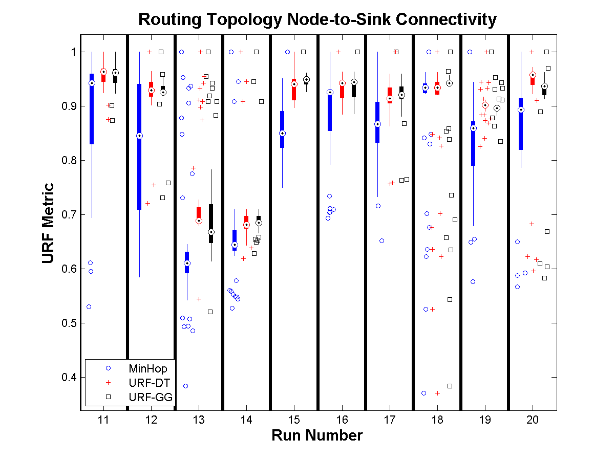
(a)

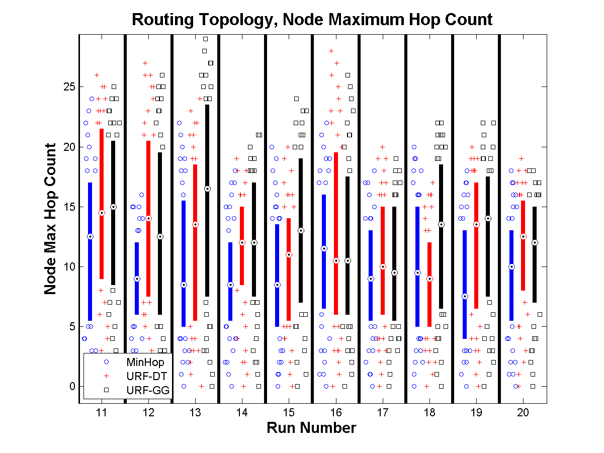
(b)

Figure 8: Comparison of routing topologies generated by MinHop, URF-DT, and URF-GG, using the LABEL:sub@fig:DAG_batch_comp_URF URF metric $\varrho_{v\rightarrow b}$ and LABEL:sub@fig:DAG_batch_comp_MaxHop maximum hop count on each node. The distributions are represented by box and whiskers plots, where the median is represented by a circled black dot, the outliers are represented by points, and the interquartile range (IQR) is 1.5 for LABEL:sub@fig:DAG_batch_comp_URF and 0 for LABEL:sub@fig:DAG_batch_comp_MaxHop.

TABLE I: MinHop, URF-DT, URF-GG Routing Topology Statistics over 100 Random Graphs

Routing	URF Metric $\varrho_{v\rightarrow b}$			Max Hop Count
Topology	mean	median	variance	mean	median
MinHop	0.8156	0.8252	0.0075	10.50	10.59
URF-DT	0.8503	0.8539	0.0041	11.41	11.68
URF-GG	0.8529	0.8549	0.0039	12.38	12.76

While in some runs the URF-DT topology shows marginal improvements in reliability over the MinHop topology, other runs (like run 17) show a significant improvement. Figure 8b shows that this often comes at the cost of increasing the maximum hop count on some of the nodes (though not always, as shown by run 17).

VIII Conclusions

Both the FPP and URF metrics show that multiple interleaved paths typically provide better end-to-end reliability than disjoint paths. Furthermore, since they were derived directly from link probabilities, the DAG representing the routing topology, and simple packet forwarding models, they help us understand when a network is reliable. Using these routing topology metrics a network designer can estimate whether a deployed network is reliable enough for his application. If not, he may place additional relay nodes to add more links and paths to the routing topology. He may also use these metrics to quickly compare different routing topologies and develop an intuition of which ad-hoc placement strategies generate good connectivity graphs.

These metrics provide a starting point for designing routing protocols that try to maintain and optimize a routing topology. The URF-DT algorithm describes how to build a reliable static routing topology, but it would be interesting to study algorithms that gradually adjusts the routing topology over time as the link estimates change.

$$\varpi_{uv} =\sum_{{\mathcal{E}}^{\prime}\in 2^{{\mathcal{E}}_{u}\backslash l}}\frac{p_{l}}{|{\mathcal{E}}^{\prime}|+1}\left(\prod_{e\in{\mathcal{E}}^{\prime}}p_{e}\right)\left(\prod_{\bar{e}\in{\mathcal{E}}_{u}\backslash({\mathcal{E}}^{\prime}\cup l)}1-p_{\bar{e}}\right)$$

$$=p_{l}\sum_{{\mathcal{E}}^{\prime}\in 2^{{\mathcal{E}}_{u}\backslash l}}\frac{1}{|{\mathcal{E}}^{\prime}|+1}\left(\prod_{e\in{\mathcal{E}}^{\prime}}p_{e}\right)\left(\prod_{\bar{e}\in{\mathcal{E}}_{u}\backslash({\mathcal{E}}^{\prime}\cup l)}1-p_{\bar{e}}\right)$$

$$=p_{l}\int_{0}^{1}\sum_{{\mathcal{E}}^{\prime}\in 2^{{\mathcal{E}}_{u}\backslash l}}\left(\prod_{e\in{\mathcal{E}}^{\prime}}p_{e}\right)\left(\prod_{\bar{e}\in{\mathcal{E}}_{u}\backslash({\mathcal{E}}^{\prime}\cup l)}1-p_{\bar{e}}\right)x^{|{\mathcal{E}}^{\prime}|}dx$$

$$=p_{l}\int_{0}^{1}\prod_{e\in{\mathcal{E}}_{u}\backslash l}\left((1-p_{e})+p_{e}x\right)dx$$

$$=p_{l}\int_{0}^{1}\prod_{e\in{\mathcal{E}}_{u}\backslash l}\left(1-p_{e}(1-x)\right)dx$$

$$=p_{l}\int_{0}^{1}\prod_{e\in{\mathcal{E}}_{u}\backslash l}\left(1-p_{e}x\right)dx$$

References

- [1] J. P. Hespanha, P. Naghshtabrizi, and Yonggang Xu, “A survey of recent results in networked control systems,” Proceedings of the IEEE, vol. 95, pp. 138–162, 2007.
- [2] Wireless Industrial Networking Alliance (WINA), “WINA website,” http://www.wina.org.
- [3] K. Pister, P. Thubert, S. Dwars, and T. Phinney, “Industrial Routing Requirements in Low-Power and Lossy Networks,” RFC 5673 (Informational), Internet Engineering Task Force, Oct. 2009. [Online]. Available: http://www.ietf.org/rfc/rfc5673.txt
- [4] D. Chen, M. Nixon, and A. Mok, WirelessHART: Real-time Mesh Network for Industrial Automation. Springer, 2010.
- [5] International Society of Automation, “ISA-SP100 wireless systems for automation website,” http://www.isa.org/isa100.
- [6] H. Dubois-Ferriere, M. Grossglauser, and M. Vetterli, “Valuable detours: Least-cost anypath routing,” IEEE/ACM Trans. on Networking, 2010, preprint, available online at IEEE Xplore.
- [7] M. E. M. Campista et al., “Routing metrics and protocols for wireless mesh networks,” IEEE Network, vol. 22, no. 1, pp. 6–12, Jan.–Feb. 2008.
- [8] T. Cormen, C. Leiserson, and R. Rivest, Introduction to Algorithms. Cambridge, Massachusetts: MIT Press, 1990.
- [9] S. De, C. Qiao, and H. Wu, “Meshed multipath routing with selective forwarding: an efficient strategy in wireless sensor networks,” Computer Networks, vol. 43, no. 4, pp. 481–497, 2003.
- [10] F. Ye, G. Zhong, S. Lu, and L. Zhang, “GRAdient Broadcast: a robust data delivery protocol for large scale sensor networks,” Wireless Networks, vol. 11, no. 3, pp. 285–298, 2005.
- [11] S. Biswas and R. Morris, “Opportunistic routing in multi-hop wireless networks,” SIGCOMM Computer Communication Review, vol. 34, no. 1, pp. 69–74, 2004.
- [12] P. Chen and S. Sastry, “Latency and connectivity analysis tools for wireless mesh networks,” in Proc. of the 1st International Conference on Robot Communication and Coordination (ROBOCOMM), October 2007.
- [13] K. S. J. Pister and L. Doherty, “TSMP: Time synchronized mesh protocol,” in Proc. of the IASTED International Symposium on Distributed Sensor Networks (DSN), November 2008.
- [14] P. Soldati, H. Zhang, Z. Zou, and M. Johansson, “Optimal routing and scheduling of deadline-constrained traffic over lossy networks,” in Proc. of the IEEE Global Telecommunications Conference (GLOBECOMM), Miami FL, USA, Dec. 2010.
- [15] Z. Zou, P. Soldati, H. Zhang, and M. Johansson, “Delay-constrained maximum reliability routing over lossy links,” in Proc. of the IEEE Conference on Decision and Control (CDC), Dec. 2010.
- [16] J. L. Sobrinho, “Algebra and algorithms for QoS path computation and hop-by-hop routing in the Internet,” IEEE/ACM Trans. on Networking, vol. 10, no. 4, pp. 541–550, Aug. 2002.
- [17] R. Bhandari, “Optimal physical diversity algorithms and survivable networks,” in Proc. of the 2nd IEEE Symposium on Computers and Communications (ISCC), Jul. 1997, pp. 433–441.
- [18] Internet Engineering Task Force, “Routing protocol for low power and lossy networks (RPL),” http://www.ietf.org/id/draft-ietf-roll-rpl-19.txt, 2011.
- [19] N. Baccour et al., “A comparative simulation study of link quality estimators in wireless sensor networks,” in IEEE International Symposium on Modeling, Analysis, and Simulation of Computer and Telecommunication Systems (MASCOTS), Sep. 2009, pp. 1–10.
- [20] P. Chen, “Wireless sensor network metrics for real-time systems,” Ph.D. dissertation, EECS Department, University of California, Berkeley, May 2009. [Online]. Available: http://www.eecs.berkeley.edu/Pubs/TechRpts/2009/EECS-2009-75.html