Detecting the optimal number of communities in complex networks

Abstract

To obtain the optimal number of communities is an important problem in detecting community structure. In this paper, we extend the measurement of community detecting algorithms to find the optimal community number. Based on the normalized mutual information index, which has been used as a measure for similarity of communities, a statistic $\Omega(c)$ is proposed to detect the optimal number of communities. In general, when $\Omega(c)$ reaches its local maximum, especially the first one, the corresponding number of communities c is likely to be optimal in community detection. Moreover, the statistic $\Omega(c)$ can also measure the significance of community structures in complex networks, which has been paid more attention recently. Numerical and empirical results show that the index $\Omega(c)$ is effective in both artificial and real world networks.

1 Introduction

Community detection has become a very important part of researches on complex networks [1, 2, 3]. Communities or modules mean high concentrations of edges within special groups of vertices, and low concentrations between these groups [4, 5, 6, 7]. Such communities have been observed in many different fields. For instance, community structure is a typical feature in social networks, where some of the individuals can be part of a tightly connected group, others can be completely isolated, while some others may act as bridges between groups. Tightly connected groups of nodes in the World Wide Web often correspond to pages on common topics, while communities in genetic networks are related to functional modules. Consequently, finding the communities within a network is a powerful tool for understanding the structure and the function of the network, and its growth mechanisms[3].

The general aim of community detection is to find meaningful divisions into groups by investigating the structural properties of the whole graph. There are two major aspects about this problem. One concerns with proposing effective algorithms for detecting the communities, and the other concerns with the significance or robustness of the obtained divisions[3, 8]. For the first aspect, many efficient heuristic methods have been proposed over the years to detect the communities in networks, in particular those based on spectral methods, divisive algorithms, modularity-based methods, dynamic algorithms, and many others. However, most existing algorithms are not able to get the optimal number directly. Communities are just the final product of the algorithm. The community number of each run may be different. For some previous algorithms which can get the ”optimal” community number depend on modularity Q, including Greedy techniques, Simulated annealing, Extremal optimization, Spectral optimization etc. By assumption, high values of modularity indicate good partitions. So, the partition corresponding to maximum value on a given graph should be the best, or at least a good one. This is the main motivation for modularity maximization, perhaps the most popular class of methods to detect communities in graphs. However, exhaustive optimization of Q is impossible, due to the maximum is out of reach, as it has been proved that modularity optimization is an NP-complete problem [9], so it is probably impossible to find the solution in a time growing polynomially with the size of the graph. Moreover, Santo et al. have been strictly proved that even if modularity Q can get the maximum value, the corresponding community number may not be the optimal one[10]. Most importantly, small changes of the number of communities may have a huge impact on the results of detecting the community structure. Therefore, it is essential to look for simple and effective methods of detecting the optimal number of communities.

When we proceed the methods several times under the same condition, they may give different community structures due to the random factors in the algorithm. Then evaluating the quality of a partition is also important in community identification. Newman described a method to calculate the sensitivity of algorithms[11]. Danon et al. proposed a measurement based on information theory [12]. These two measurements mainly focus on the proportion of nodes which are correctly grouped. Fan et al. investigated the accuracy and precision of several algorithms [13]. Accuracy means the consistence when the community structure from algorithm is compared with the presumed communities, and precision is the consistence among the community structures from different runs of an algorithm on the same network. They proposed a similarity function S to measure the difference between partitions. The function S integrates the information about the proportion of nodes co-appearance in pair groups of A, B and the total number of communities. Obviously, an ”ideal” community detection should be one that both with high accuracy and high precision. In this paper, we propose a suitable method for evaluating the optimal number of the communities based on measuring the precision of algorithms and closely relating to the accuracy of algorithms. We first use the algorithm based on mixture model,which proposed by Newman and Leicht[14], to induce a sequence $P(k)(1\leq{k}\leq{n})$ of divisions into communities; Second, we measure the precision of the algorithm based on ”information entropy”, which has been used to evaluate the similarity of communities[15, 16, 17, 18]; At last, we use our proposed index $\Omega(c)$ to find the optimal number of the communities. Our statistic is an auxiliary method which can be applied to almost all the algorithms with random characteristics to help them find the optimal community number. It is relatively simple to apply the method. It will not increase the complexity of the algorithms, which just repeat the algorithm for several times. A point we should mention is that our method needn’t to know the ”real” community structures in advance.

This paper is organized as follows: The method is described in detail in section 2. In section 3, we apply the method to several artificial and real networks, and find some interesting results. In section 4, some conclusions are given.

2 Method

First, for given number of groups c, we use the method based on mixture model to divide a network n times, then we can get n (in this paper, $\emph{n}=50$) divisions of the same network into communities. When we proceed the method several times under the same condition, they may give different community structures due to the random factors of the algorithm. So these divisions generally have different community structures, meaning that the communities in different divisions may include different nodes and edges.

Second, we measure the precision of the algorithm based on comparing the similarity between the divisions. A number of indexes for measuring similarities or differences between partitions of a network have been proposed in the past [13, 15, 16, 17, 18, 19, 20, 21]. Our method here follows the information theoretic methods. As described in Ref.[12, 15], a confusion matrix N was defined, where the rows correspond to the ”real” communities in networks, and the columns correspond to the ”found” communities. The element $N(i,j)$ is the number of nodes in the real community i that appear in the found community j. Therefore a measure of similarity between the partitions A and B is

$$R(c)=I{(A,B)}=\frac{-2\sum_{i=1}^{c_{A}}\sum_{j=1}^{c_{B}}N_{ij}log{(\frac{N_{ij}N}{N_{i.}N{.j}})}}{\sum_{i=1}^{c_{A}}N_{i.}log{(\frac{N_{i.}}{N})}+\sum_{j=1}^{c_{B}}N_{.j}log{(\frac{N_{.j}}{N})}}$$ (1)

Where A is the ”real” community structure of the network, B denotes the divisions of the network, and $c_{A}$, $c_{B}$ denote the numbers of ”real” communities and ”found” communities respectively. I(A,B) is to measure the accuracy of the algorithm. The larger I(A,B) is, the better the community structure from algorithm is consistent with the ”real” one. We assume $c_{A}=c_{B}=c$, then $I{(A,B)}$ can be simplified to

$$I_{c}{(a,b)}=\frac{-2\sum_{i=1}^{c}\sum_{j=1}^{c}N_{ij}log{(\frac{N_{ij}N}{N_{i.}N{.j}})}}{\sum_{i=1}^{c}N_{i.}log{(\frac{N_{i.}}{N})}+\sum_{j=1}^{c}N_{.j}log{(\frac{N_{.j}}{N})}}$$ (2)

Both A and B in Eq.(2) are the divisions from the different runs of an algorithm on the same network. Then $I_{c}{(a,b)}$ could measure the precision of the algorithm. Here we use Eq.(2) to compare every two different divisions of the same network into communities. Then for each given c and n, we will get $\frac{\emph{n}(\emph{n}-1)}{2}$ values of $I_{c}{(a,b)}$.

Then, we propose an index $\Omega(c)$ as following,

$$\Omega(c)=\frac{\sum_{a=1,b=1,a<b}^{n}I_{c}{(a,b)}}{\frac{n(n-1)}{2}}=\frac{2}{n(n-1)}\sum_{a=1,b=1,a<b}^{n}I_{c}{(a,b)}$$ (3)

$\Omega(c)$, actually, can also measure the precision of the algorithms.

To show the effectiveness of our index $\Omega(c)$, we compare it with $R(c)$ in a variety of networks whose community structures are known. In general, the number of communities is much smaller than the number of nodes in a network. Then, when the number of communities is far fewer than the number of nodes, we find that $\Omega(c)$ performs as well as $R(c)$ in measuring the similarities between community structures. And we find that when it appears local maximum, especially the first maximum, the corresponding c is likely the optimal number of groups.

3 Results

In order to investigate the performance of our index $\Omega(c)$, we compare these two indices in ad hoc networks and some real networks which have ”known” community structures. To further measure the performance of $\Omega(c)$, we apply it in several artificial hierarchical networks which have ”unknown” community structures in advance, and we compare it with function Q in ER random networks. Finally, we intend to use $\Omega(c)$ to measure the significance of community structure.

3.1 Results of Binary ad hoc networks

As a first test, we applied $\Omega(c)$ to computer-generated random graphs with a well-known predetermined community structure[22]. Each graph has $N=128$ nodes divided into $4$ communities of $32$ nodes each. Edges between two nodes are introduced with different probabilities depending on whether the two nodes belong to the same group or not: every node has $k_{intra}$ links on average to its neighbors in the same community and $k_{inter}$ links to the outer world, keeping $<k_{intra}>$ + $<k_{inter}>$ =16. In Fig.1, we show the performs of $\Omega(c)$ and $R(c)$ in several Binary ad hoc networks. The curves correspond to different choices for different $<k_{intra}>$. As we can see from Fig.1, $\Omega(c)$ performances as well as $R(c)$, and when $\Omega(c)$ reaches the first maximum value, the corresponding number of groups $c=4$ is the optimal number of communities.

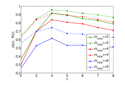
Figure 1: Comparing $\Omega(c)$ (shown with real lines) and $R(c)$ (shown with broken lines) in ad hoc networks with $n=128$, and 4 communities of 32 nodes each. The X axis denotes the number of communities. The plot shows the results for three different numbers of $<k_{intra}>$ corresponding to 2, 4, or 6. Both $\Omega(c)$ and $R(c)$ achieve their first maximum when the number of communities is 4. The result is averaged by 100 times.

3.2 Results on Zachary’s karate club network

The Zachary karate club network has been considered as a simple sample for community-detecting methodologies[14, 22, 23, 24, 25, 26, 27]. This network is constructed with the data collected from observing $34$ members of a karate club over a period of 2 years and considering friendship between members. It has been proved that the best partition of this network has two communities by many previous algorithms[7, 14, 15, 22]. We also apply $\Omega(c)$ and $R(c)$ to the Zachary karate club network. As shown in Fig.2, $\Omega(c)$ appears its first maximum value when c=2. According to our method, $c=2$ is the optimal number of communities in the Zachary karate club network, which correspond to the results given in[7, 14].

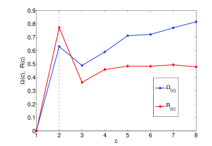
Figure 2: Comparing $\Omega(c)$ (shown with square line) and $R(c)$ (shown with diamond line) in the Zachary’s karate club network. Both of them achieve the first maximum when the number of communities is 2. The result is averaged by 100 times.

3.3 Results on an LFR Benchmark

As we have remarked above, all vertices of ad hoc networks have approximately the same degree and all communities have exactly the same size by construction. These two features are at odds with what is observed in graph representations of real systems. Degree distributions of real networks are usually skewed, with many vertices with low degree coexisting with a few vertices with high degree. Lancichinetti, Fortunato, and Radicchi considered that a good benchmark should not be assumed that all communities have the same size: the distribution of community sizes of real networks is also broad, with a tail that can be fairly well approximated by a power law. They introduced a class of benchmark graphs which account for the heterogeneity in the distributions of both degree and community size[28, 29]. Such benchmark is a more faithful approximation of real-world networks with community structure than simpler benchmarks like, e. g. that by Girvan and Newman. Through the method in[28], we get a class of LFR Benchmark networks and we apply index $\Omega(c)$ to one of them. The result is shown in Fig.3. As we can see from the figure, when $c=10$, $\Omega(c)$ reaches the first maximum value, which corresponds to the condition of the network we construct. In fact, $\Omega(c)$ relates to the number of communities. When the community number c is large enough, $\Omega(c)$ is bound to increase with the increase of c. When the community number is equal to the network size, $\Omega(c)$ will be one. Our statistic is generally effective on the networks which their community number is much smaller than the vertex number, which is consistent with the characteristic of most real networks.

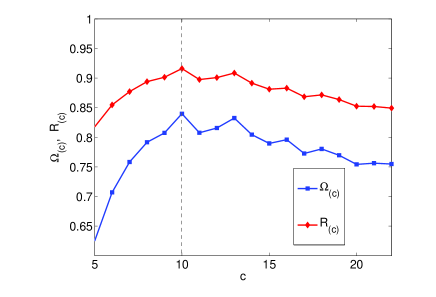
Figure 3: Comparing $\Omega(c)$ (shown with square line) and $R(c)$ (shown with diamond line) in one of LFR benchmark networks, which has a skewed degree distribution, similar to real networks. The number of nodes N=500; Each node is given a degree taken from a power law distribution with exponent $\gamma$=3; The average node degree $<k>$=20; Each node shares a fraction $1-\mu$ of its links with the other nodes of its community and a fraction $\mu$ with the other nodes of the network; $\mu$=0.2 is the mixing parameter; The sizes of the communities are taken from a power law distribution with exponent $\beta$=2. Through the method, we get the network and the number of communities $c$=10. Both $\Omega(c)$ and $R(c)$ appear the first local maximum value when the number of communities is 10.

3.4 Results on hierarchical networks

Hierarchical networks have been mentioned in many literatures [30, 31, 32, 33, 34, 35]. Marta Sales-Pardo et al. proposed a method to construct hierarchical nested random graphs[34]. In this paper, we test our method on hierarchical artificial networks with two levels. Taking Fig.4(a) as an example, we explain how we construct the hierarchical networks. We first create a network with 80 nodes that at the first level has two modules comprising 40 nodes each. Once having assigned nodes to groups, we draw an edge between a pair of nodes $(i,j)$ with probabilities

(1.) $p_{2}$($p_{2}=\frac{d_{2}}{c_{2}}$), where $d_{2}$ is the average degree of the module at the second level and $c_{2}$ is the number of nodes in the module), if $(i,j)$ are in the same module at the second level; (2.) $p_{1}$($p_{1}=\frac{d_{1}}{c_{1}}$), where $d_{1}$ is the average degree of the module at the first level and $c_{1}$ is the number of nodes in the module), if $(i,j)$ are in the same module at the first level; (3.) $p_{0}$($p_{0}=\frac{d_{0}}{c_{0}}$), where $d_{0}$ is the average degree of the module at the top level and $c_{0}$ is the number of nodes in the whole network, otherwise. We impose that $p_{2}>p_{1}>p_{0}$ (here $p_{2}=0.85$, $p_{1}=0.25$, $p_{0}=0.01$), then the resulting network has a larger density of connections between nodes grouped in the same submodule at the second level, a smaller density of connections between groups of nodes grouped in the same module at the first level, and an even smaller density of connections between nodes grouped in separate modules at the top level. Thus, the network has by construction an artificial hierarchical organization. Fig. 4 shows the results of $\Omega(c)$ in two of these kinds of networks. In Fig.4, $\Omega(c)$ appears several local maximum values, and we can find that the corresponding numbers of communities of the first two maximum values of $\Omega(c)$ are well corresponding to the number of communities of different levels in hierarchical networks. However, $\Omega(c)$ can not always detect the ”optimal” community number of hierarchical networks effectively, but just with a certain probability. For example, we have calculated the probabilities of the above two hierarchical networks. For the 80-nodes network, the probabilities of obtaining a maximum when c=2 and c=4 are 0.91, 0.32 respectively. For the 180-nodes network, the probabilities of obtaining a maximum when c=3 and c=9 are 0.85, 0.21 respectively. What’s more, as shown in fig.4(b), $\Omega(2)>\Omega(4)$; and as shown in fig.4(d), $\Omega(3)>\Omega(9)$. This is a very interesting phenomenon, which means large community structures are more likely to be identified by the algorithms.

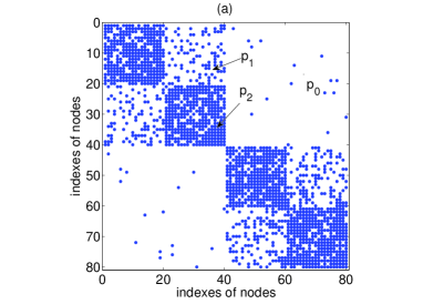
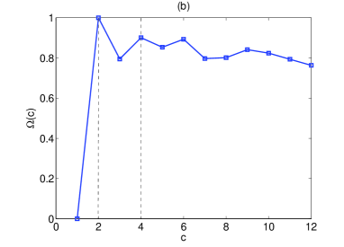
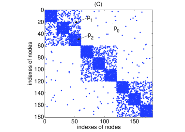
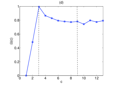
Figure 4: The performance of $\Omega(c)$ in computer-generated hierarchical networks. In (a), (c), both the x axis and the y axis present the number of nodes n in the networks. In (b), (d), the x axis presents the number of communities. From the plots we can see that our method is also helpful for detecting the community structures at different levels in artificial hierarchical networks. (a) $n=80$, $p_{0}=0.002$, $p_{1}=0.1$, $p_{2}=0.85$; (c) $n=180$, $p_{0}=0.005$, $p_{1}=0.2$, $p_{2}=0.8$;

3.5 Results on an ER random network

Ref.[8, 36, 37] show that high values of the modularity of Newman and Girvan does not necessarily indicate that a graph has a definite cluster structure. It in particular shows that partitions of random graphs may also achieve considerably large values of Q, although we do not expect them to have community structure, due to the lack of correlations between the linking probabilities of the vertices. We compare the index $\Omega(c)$ with the modularity function Q in an ER network, which have $128$ nodes and $<k>=1.5$. The network is normally considered with indefinite community structure. We use the extremal optimization algorithm[25] to detect the community structure of the network. It is divided into $14$ communities and the maximal Q is 0.6056, which is large enough to consider the network has definite community structure. It means the modularity function Q doesn’t performs well in networks which have indefinite community structures. We apply $\Omega(c)$ to the network. As shown in Fig.5, the statistic $\Omega(c)$ doesn’t appear maximums. According to our method, it can’t find the optimal number of communities in the network, meaning that the network doesn’t have definite community structure. Thus $\Omega(c)$ may shed light on evaluating whether a network has definite community structure or not.

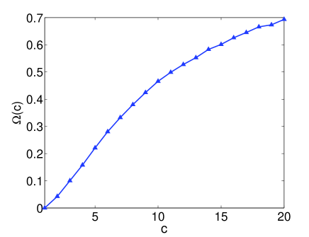
Figure 5: The performance of $\Omega(c)$ in an ER random network, which has N=128 nodes and $<k>=1.5$. This random network is normally considered with no definite community structure. However, the maximum of modularity function Q calculated by extremal optimization algorithm is 0.6056, which is large enough to consider the network has definite community structure. $\Omega(c)$ doesn’t appear maximums. It means that the network doesn’t have definite community structure, which correspond with the real condition. The result is averaged by 100 times.

3.6 Measuring the significance of community structures

Many efficient methods have been proposed for finding communities, but few of them can evaluate the communities found are significant or trivial definitely[16]. In some works the concept of significance has been related to that of robustness or stability of a partition against random perturbations of the graph structure. The basic idea is that, if a partition is significant, it will be recovered even if the structure of the graph is modified, as long as the modification is not too extensive. Instead, if a partition is not significant, one expects that minimal modifications of the graph will suffice to disrupt the partition, so other clusterings are recovered[8]. We apply the statistic $\Omega(c)$ to evaluate the significance of communities in binary ad hoc networks. As described in $3.1$, each of these computer-generated networks has $N=128$ nodes divided into $4$ communities of $32$ nodes each and we know the optimal number of communities of them is $4$. By treating $c=4$, we apply $\Omega(4)$ and $R(4)$ to measure the significance of these networks. With $<k_{intra}>$ increasing, the community structure of the network will become less and less significative. As shown in Fig.6, both $\Omega(4)$ and $R(4)$ are descending with the increase of $<k_{intra}>$, which indicates $\Omega(c)$ performs well in measuring the significance of community structures in complex networks.

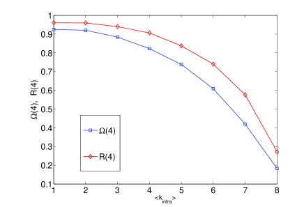
Figure 6: The performance of $\Omega(c)$ (shown with blue square line) and $R(c)$ (shown with red diamond line) in measuring the significance of community structures in computer-generated networks. Both $\Omega(c)$ and $R(c)$ are descending with the increase of $<k_{intra}>$ due to the community structures becoming fuzzier and fuzzier. The X axis gives the change of $<k_{intra}>$. The result is averaged by 100 times.

4 Conclusion and Discussion

The investigation of the optimal number of communities in a network is an important and tough issue in the study of complex networks. In this paper, we present a method to detect the optimal number of communities in complex networks based on the information theoretic ideas. We apply the index $\Omega(c)$ to some networks,including artificial networks and real networks with well-known community structures. The results show that when the number of communities is much smaller than the number of nodes, the index is effective on normal networks, LFR benchmark networks and hierarchical community structure networks. For hierarchical networks, $\Omega(c)$ can just detect the ”optimal” community number of hierarchical networks with a certain probability and we have found a very interesting phenomenon, which large community structures are more likely to be identified by the algorithms. This phenomenons will be further considered in our future work. Moreover, the index $\Omega(c)$ can be used to measure the significance of community structure which has been paid much attention recently. The statistic can nearly work based on every community detecting algorithm with the character of randomization, and it will not change the complexity of the algorithm.

References

- [1] R. Albert and A.-L. Barabasi, Rev. Mod. Phys. 74,47 (2002).
- [2] M. E. J. Newman. Phys. Rev. E 68, 026121 (2003).
- [3] S. Boccalettia, V. Latorab, Y. Morenod, M. Chavezf and D.-U. Hwanga. Physics Report 424 175 (2006).
- [4] M. E. J. Newman. SIAM REVIEW 45, 167 (2003).
- [5] F. Radicchi, C. Castellano, F. Cecconi, V. Loreto and D. Parisi. Proc. Natl. Acad. Sci. U.S.A. 101, 2658 (2004).
- [6] M. Girvan and M. E. J. Newman. Phys. Rev. E 70, 066111 (2004).
- [7] M. E. J. Newman. Proc. Natl. Acad. Sci. U.S.A. 103, 8577 (2006).
- [8] S. Fortunato. Physics Reports 486, 75 (2010).
- [9] U. Brandes, D. Delling, M. Gaertler, R. Gorke, M. Hoefer, Z. Nikoloski and D. Wagner. URL 001907 (2006).
- [10] S. Fortunato and M. Barthe. Proc. Natl. Acad. Sci. U.S.A. 104, 36 (2007).
- [11] M. E. J. Newman. Phys. Rev. E 69, 066133 (2004).
- [12] L. Danon, A. D az-Guilera, J. Duch and A. Arenas. Journal of Statistical Mechanics:Theory and Experiment P09008 (2005).
- [13] Y. Fan, M. Li, P. Zhang, J. Wu and Z. Di. Physica A 377, 363 (2007).
- [14] M. E. J. Newman and E. A. Leicht. Proc. Natl. Acad. Sci. U.S.A. 9564 (2007).
- [15] L. Donetti and M. A. Munoz. Journal of Statistical Mechanics: Theory and Experiment P10012 (2004).
- [16] Y. Hu, Y. Nie, H. Yang, J. Cheng, Y. Fan and Z. Di. Phys. Rev. E 82, 066106 (2010).
- [17] M. Meila. Journal of Multivariate Analysis 98, 873 (2007).
- [18] B. Karrer, E. Levina and M. E. J. Newman. Phys. Rev. E 77, 046119 (2008).
- [19] J. Reichardt and M. Leone. Phys. Rev. Lett. 101, 078701 (2008).
- [20] G. Bianconi, P. Pin and M. Marsili. Proc. Natl. Acad. Sci. U.S.A. 106, 11433 (2009).
- [21] D. Gfeller, J. Chappelier and P. De Los Rios. Phys. Rev. E 72, 056135 (2005).
- [22] M. E. J. Newman and M. Girvan. Phys. Rev. E 69, 026113 (2004).
- [23] Y. Hu, M. Li, P. Zhang, Y. Fan and Z. Di. Phys. Rev. E 78, 016115 (2008).
- [24] P. Pons and M. Latapy. Journal of Graph Algorithms and Applications 10, 191 (2006).
- [25] J. Duch and A. Arenas. Phys. Rev. E 72, 027104 (2005).
- [26] J. P. Bagrow and E. M. Bollt. Phys. Rev. E 72, 046108 (2005).
- [27] Y. Hu, J. Wu and Z. Di. Europhys. Lett. 85, 18009 (2009).
- [28] A. Lancichinetti, S. Fortunato and F. Radicchi. Phys. Rev. E 78, 046110 (2008).
- [29] A. Lancichinetti and S. Fortunato. Phys. Rev. E 80, 016118 (2009).
- [30] J. Reichardt and S. Bornholdt. Phys. Rev. E 74, 016110 (2006).
- [31] A. Clauset, C. Moore and M. E. J. Newman. Nature 453, 98 (2008).
- [32] N. Kashtan and U. Alon. Proc. Natl. Acad. Sci. U.S.A. 102, 13773 (2005).
- [33] S. Itzkovitz, R. Levitt, N. Kashtan, R. Milo, M. Itzkovitz and U. Alon. Phys. Rev. E 71, 016127 (2005).
- [34] M. Sales-Pardo, R. Guimera, A. A. Moreira and L. A. N. Amaral. Proc. Natl. Acad. Sci. U.S.A. 104, 15224 (2007).
- [35] X. Cheng and H. Shen. Journal of Statistical Mechanics:Theory and Experiment. P04024 (2010).
- [36] A. Lancichinetti, F. Radicchi and J. J. Ramasco. Phys. Rev. E 81, 046110 (2010)
- [37] F. Radicchi, A. Lancichinetti and J. J. Ramasco. Phys. Rev. E 82, 026102 (2010).