Electromagnetic Casimir Forces of Parabolic Cylinder and Knife–Edge Geometries

Abstract

An exact calculation of electromagnetic scattering from a perfectly conducting parabolic cylinder is employed to compute Casimir forces in several configurations. These include interactions between a parabolic cylinder and a plane, two parabolic cylinders, and a parabolic cylinder and an ordinary cylinder. To elucidate the effect of boundaries, special attention is focused on the “knife-edge” limit in which the parabolic cylinder becomes a half-plane. Geometrical effects are illustrated by considering arbitrary rotations of a parabolic cylinder around its focal axis, and arbitrary translations perpendicular to this axis. A quite different geometrical arrangement is explored for the case of an ordinary cylinder placed in the interior of a parabolic cylinder. All of these results extend simply to nonzero temperatures.

I Introduction

The Casimir force, arising from quantum fluctuations of the electromagnetic field in vacuum, is a striking manifestation of quantum field theory at the mesoscopic scale. Casimir’s computation of the force between two parallel metallic plates Casimir48 gives the classic demonstration of this phenomenon. Following its experimental confirmation in the past decade experiments , however, the Casimir force is now important to the design of microelectromechanical systems MEMS . Potential practical applications have motivated the development of large-scale numerical methods to compute Casimir forces for objects of any shape Johnson ; worldline ; Maggs . In contrast, the simplest and most commonly used analytic methods for dealing with complex shapes, such as the proximity force approximation (PFA), rely on pairwise summations, limiting their applicability.

Recently we have developed a formalism spheres ; universal that relates the Casimir interaction among several objects to the scattering of the electromagnetic field from the objects individually. This method decomposes the path integral representation of the Casimir energy GK as a log-determinant Klich in terms of a multiple scattering expansion, as was done for asymptotic separations in Ref. Balian . It can also be regarded as a concrete implementation of the perspective emphasized by Schwinger Schwinger75 that the fluctuations of the electromagnetic field can be traced back to charge and current fluctuations on the objects. (For additional perspectives on the scattering formalism, see also references in universal .) This approach allows us to take advantage of the well-developed machinery of scattering theory. In particular, the availability of exact scattering amplitudes for simple objects, such as spheres and cylinders, has made it possible to compute the Casimir force for two spheres spheres , a sphere and a plate sphere+plate , multiple cylinders cylinders , and cases with more than two objects JamalAlejandro ; Maghrebi . This formalism has also been applied and extended in a number of other situations Johnson ; Kenneth ; Milton ; Golestanian ; Ttira .

Here we expand on recent work paraboloid that showed how to apply these techniques to parabolic cylinders, another example where the scattering amplitudes can be computed exactly. The limiting case when the radius of curvature at the tip vanishes, so that the parabolic cylinder becomes a semi-infinite plate (a “knife-edge”), provides a particularly interesting application of this approach. One can also model the knife-edge as the limit of a wedge of zero opening angle sharp ; the two approaches are rather complementary as the former is most amenable to numerical computation, while the latter yields approximate analytic formulae via a multiple reflection expansion (which is useful for other sharp geometries, such as the cone sharp ). Edge geometries have also been considered in Refs. Gies ; Kabat .

The remainder of the manuscript is organized as follows: The Helmholtz equation in the parabolic cylinder coordinate system is reviewed in Sec. II, and exact formulae are derived for the scattering of the electromagnetic field from a perfectly conducting parabolic cylinder. The techniques of Refs. spheres ; universal , are then employed to find the electromagnetic Casimir interaction energy for a variety of situations: We let the parabolic cylinder interact with a plane (Sec. III), a second parabolic cylinder (Sec. IV), or an ordinary cylinder (Sec. V). In these calculations we consider arbitrary rotations of the parabolic cylinder around its focal axis and arbitrary translations perpendicular to that axis, transformations that are particularly useful when considering the “knife-edge” limit. We also position an ordinary or parabolic cylinder inside a parabolic cylinder (Sec. VI), and incorporate the effects of thermal corrections in all of these calculations (Sec. VII).

II Scattering in Parabolic Cylinder Coordinates

We begin with a review of scattering theory in parabolic cylinder coordinates MF ; WW . Because the system is translationally invariant in the $z$ direction and perfectly reflecting, we can decompose the electromagnetic scattering problem into two scalar problems, one with Dirichlet and the other with Neumann boundary conditions. Parabolic cylinder coordinates are defined by

$$x=\mu\lambda\,,\qquad y=\frac{1}{2}(\lambda^{2}-\mu^{2})\,\qquad z=z\,,$$ (1)

such that for $r=\sqrt{x^{2}+y^{2}}$,

$$\lambda={\rm sgn}(x)\sqrt{r+y}\,\qquad\mu=\sqrt{r-y}\,,$$ (2)

where we have chosen a convention where $\mu\geq 0$ but $\lambda$ can have either sign, which is explained in more detail below. This restricted domain is sufficient to include all points in space. Note that here we must take ${\rm sgn}(0)=1$, not ${\rm sgn}(0)=0$. At fixed $z$, the surfaces of constant $\mu$ are confocal parabolas opening upward (toward positive $y$) and the surfaces of constant $\lambda$ are confocal parabolas opening downward (toward negative $y$), as shown in Fig. 1. The scale factors (metric coefficients) are $h_{\lambda}=h_{\mu}=\sqrt{\lambda^{2}+\mu^{2}}$, $h_{z}=1$.

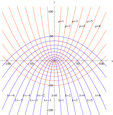
Figure 1: Coordinate curves in parabolic cylinder coordinates.

We would like to solve the Helmholtz equation, which in these coordinates takes the form

$$\nabla^{2}\Phi(\bm{r})=\frac{1}{\lambda^{2}+\mu^{2}}\left(\frac{d^{2}\Phi}{d\lambda^{2}}+\frac{d^{2}\Phi}{d\mu^{2}}\right)+\frac{d^{2}\Phi}{dz^{2}}=-k^{2}\Phi(\bm{r})\,,$$ (3)

where eventually we will set $k=i\kappa$. For $k$ real, we expect oscillating traveling wave solutions, while for $\kappa$ real, we expect exponentially growing and decaying solutions. This equation is amenable to separation of variables:

$$\Phi(\lambda,\mu,z)=L(\lambda)M(\mu)Z(z)\,.$$ (4)

Separation of the $z$ variable is trivial, $Z(z)=e^{ik_{z}z}$, leaving

$$\frac{1}{L}\frac{d^{2}L}{d\lambda^{2}}+\frac{1}{M}\frac{d^{2}M}{d\mu^{2}}=(k_{z}^{2}-k^{2})(\lambda^{2}+\mu^{2})\,,$$ (5)

which gives the separated equations

$$\frac{d^{2}L}{d\lambda^{2}}-(k_{z}^{2}-k^{2})\lambda^{2}L = -qL\,,$$ (6)

$$\frac{d^{2}M}{d\mu^{2}}-(k_{z}^{2}-k^{2})\mu^{2}M = qM\,,$$ (7)

where $q$ is a separation constant. The solutions are

$$L(\lambda)=D_{\nu}(\tilde{\lambda}) L(\lambda)=D_{-\nu-1}(i\tilde{\lambda})\,,$$ and (8)

$$M(\mu)=D_{\nu}(i\tilde{\mu}) M(\mu)=D_{-\nu-1}(\tilde{\mu})\,,$$ and (9)

in terms of the parabolic cylinder function $D_{\nu}(u)$. Here

$$\tilde{\lambda} = \lambda\sqrt{-2i\sqrt{k^{2}-k_{z}^{2}}}=\lambda\sqrt{2\sqrt{k_{z}^{2}+\kappa^{2}}}\,,$$ (10)

$$\tilde{\mu} = \mu\sqrt{-2i\sqrt{k^{2}-k_{z}^{2}}}=\mu\sqrt{2\sqrt{k_{z}^{2}+\kappa^{2}}}\,,$$ (11)

and

$$\nu=\frac{1}{2}\left(\frac{q}{\sqrt{k_{z}^{2}-k^{2}}}-1\right)\,,\hbox{~{}~{}~{}which implies~{}~{}~{}}-\nu-1=\frac{1}{2}\left(\frac{-q}{\sqrt{k_{z}^{2}-k^{2}}}-1\right)\,.$$ (12)

The second solution in each case is obtained by making the replacements $q\to-q$, $\lambda\to i\lambda$, and $\mu\to-i\mu$, the combination of which leaves the differential equations invariant. For $\displaystyle|\arg u|<{3\pi}/{4}$, $D_{\nu}(u)\sim u^{\nu}e^{-u^{2}/4}$ as $|u|\to\infty$. So for both $\lambda$ and $\mu$, we have solutions that both grow and decay exponentially as their argument approaches positive infinity. Since the Cartesian radial distance is $\displaystyle r=(\lambda^{2}+\mu^{2})/2$, these are ordinary exponentials (not Gaussians) when expressed in terms of Cartesian coordinates.

If we send $\lambda$ to $-\lambda$ and $\mu\to-\mu$, we return to the same point in space, so a wavefunction defined everywhere in the plane must be invariant under this transformation. From the identity

$$D_{\nu}(-\tilde{\lambda})=(-1)^{\nu}D_{\nu}(\tilde{\lambda})+\frac{\sqrt{2\pi}}{\Gamma(-\nu)}i^{\nu+1}D_{-\nu-1}(i\tilde{\lambda})\,,$$ (13)

we can conclude that $\nu$ must be a non-negative integer to satisfy this requirement. We begin with the case

$$L(\lambda)M(\mu)=D_{\nu}(\tilde{\lambda})D_{\nu}(i\tilde{\mu})\,,$$ (14)

for $\nu=0,1,2,3,\cdots$. For these values of $\nu$, the parabolic cylinder functions with real arguments are simple rescalings of the solutions to the quantum harmonic oscillator, and thus are given by a Gaussian times a Hermite polynomial. The combined solution in Eq. (14) then takes the form of a polynomial in $\mu$ and $\lambda$ times $\displaystyle e^{i\sqrt{k^{2}-k_{z}^{2}}y}$, and thus represents a traveling parabolic wave in the $+y$ direction.

These solutions represent “regular” waves, the analogs of solutions in spherical coordinates involving spherical Bessel functions and spherical harmonics, $j_{\ell}(kr)Y^{\ell}_{m}(\theta,\phi)$. Since we have chosen to restrict $\mu$ to positive values, it will represent the analog of the radial coordinate $r$. We will also require “outgoing” solutions to the same differential equations, the analogs of solutions in spherical coordinates involving spherical Hankel functions and spherical harmonics, $h^{(1)}_{\ell}(kr)Y^{\ell}_{m}(\theta,\phi)$. As in the spherical case, in the irregular solution the function of the “angular” variable $\lambda$ is the same, but the function of the “radial” variable is an independent solution to the same differential equation,

$$L(\lambda)M(\mu)=D_{\nu}(\tilde{\lambda})D_{-\nu-1}(\tilde{\mu})\,,$$ (15)

again for $\nu=0,1,2,3,\cdots$. Even though they do not blow up at $\mu=0$ (as the outgoing spherical wavefunctions do at $r=0$), these solutions are not permissible for $\mu<0$ because they are not invariant under the combined substitution $\mu\to-\mu$ and $\lambda\to-\lambda$. The solution in Eq. (15) asymptotically approaches a polynomial in $\mu$ and $\lambda$ times $\displaystyle e^{i\sqrt{k^{2}-k_{z}^{2}}r}$, and thus represents an outgoing radial parabolic wave.

We define the full regular and outgoing solutions

$$\psi_{\nu}^{\hbox{\tiny reg}}(\bm{r}) = i^{\nu}e^{ik_{z}z}D_{\nu}(\tilde{\lambda})D_{\nu}(i\tilde{\mu})\,,$$ (16)

$$\psi_{\nu}^{\hbox{\tiny out}}(\bm{r}) = e^{ik_{z}z}D_{\nu}(\tilde{\lambda})D_{-\nu-1}(\tilde{\mu})\,,$$ (17)

using which the free Green’s function becomes, for $\mu\geq 0$ MF ,

$$G(\bm{r}_{1},\bm{r}_{2},k)=\int_{-\infty}^{\infty}\frac{dk_{z}}{2\pi}\sum_{\nu=0}^{\infty}\frac{(-1)^{\nu}}{\nu!\sqrt{2\pi}}\psi_{\nu}^{\hbox{\tiny reg}}(\bm{r_{<}})^{*}\psi_{\nu}^{\hbox{\tiny out}}(\bm{r_{>}})\,.$$ (18)

Here $\bm{r}_{<}$ ($\bm{r}_{>}$) is the point with the smaller (larger) of $\mu_{1}$ and $\mu_{2}$, and we have made use of the Wronskian of the two independent solutions for each $\nu$,

$$W[D_{\nu}(u),D_{-\nu-1}(iu)]=i^{\nu-1}\,.$$ (19)

The decomposition of a plane wave in regular parabolic cylinder functions is MF

$$e^{i\bm{k}\cdot\bm{r}}=e^{ik_{z}z}\frac{1}{\cos\frac{\phi}{2}}\sum_{\nu=0}^{\infty}\frac{1}{\nu!}\left(\tan\frac{\phi}{2}\right)^{\nu}\psi_{\nu}^{\hbox{\tiny reg}}(\bm{r})\,,$$ (20)

where

$$\phi=\frac{1}{2i}\log\frac{k_{y}+ik_{x}}{k_{y}-ik_{x}}\,,$$ (21)

and $k_{y}=\sqrt{k^{2}-k_{x}^{2}-k_{z}^{2}}=i\sqrt{\kappa^{2}+k_{x}^{2}+k_{z}^{2}}$. Here the logarithm defines the arctangent of $k_{x}/k_{y}$ in the appropriate quadrant. Note that the expansion in Eq. (20) converges only for $k_{y}>0$, since it is built out of parabolic waves that propagate upward.

To determine the T-matrix we consider Dirichlet or Neumann boundary conditions at $\mu=\mu_{0}\geq 0$. In the region $\mu>\mu_{0}$ we have the scattering solution

$$\Phi(\bm{r})=\psi_{\nu}^{\hbox{\tiny reg}}(\bm{r})-i^{\nu}\frac{D_{\nu}(i\tilde{\mu}_{0})}{D_{-\nu-1}(\tilde{\mu}_{0})}\psi_{\nu}^{\hbox{\tiny out}}(\bm{r})\hbox{\qquad(Dirichlet)}$$ (22)

for Dirichlet boundary conditions and

$$\Phi(\bm{r})=\psi_{\nu}^{\hbox{\tiny reg}}(\bm{r})-i^{\nu+1}\frac{D_{\nu}^{\prime}(i\tilde{\mu}_{0})}{D_{-\nu-1}^{\prime}(\tilde{\mu}_{0})}\psi_{\nu}^{\hbox{\tiny out}}(\bm{r})\hbox{\qquad(Neumann)}$$ (23)

for Neumann boundary conditions, where prime denotes the derivative of the parabolic cylinder function with respect to its argument and $\nu=0,1,2,3,\cdots$. These wavefunctions correspond to the scattering $T$-matrix elements ${\cal T}_{\nu k_{z}\nu^{\prime}k_{z}^{\prime}}=2\pi\delta(k_{z}-k_{z}^{\prime})\delta_{\nu\nu^{\prime}}{\cal T}_{\nu}^{C}$, with

$${\cal T}_{\nu}^{C} = -i^{\nu}\frac{D_{\nu}(i\tilde{\mu}_{0})}{D_{-\nu-1}(\tilde{\mu}_{0})}\hbox{\qquad(Dirichlet),}$$ (24)

$${\cal T}_{\nu}^{C} = -i^{\nu+1}\frac{D_{\nu}^{\prime}(i\tilde{\mu}_{0})}{D_{-\nu-1}^{\prime}(\tilde{\mu}_{0})}\hbox{\qquad(Neumann),}$$ (25)

for the process where an incoming parabolic wave propagating in the $+y$ direction is scattered into an outgoing parabolic wave propagating radially.

The solutions we have obtained allowed us to construct the complete free Green’s function, the decomposition of a plane wave, and the scattering $T$-matrices, which contain all the information we will need to carry out our calculations. However, we note that there also exists a second set of solutions, representing the time-reversed scattering process,

$$L(\lambda)M(\mu)=D_{-\nu-1}(i\tilde{\lambda})D_{-\nu-1}(\tilde{\mu})\,,$$ (26)

for $\nu=0,1,2,3,\cdots$, which also are unchanged for $\lambda\to-\lambda$ and $\mu\to-\mu$. For real $k$, these solutions go like $e^{-i\sqrt{k^{2}-k_{z}^{2}}y}$ and so propagate in the $-y$ direction, in contrast to the solutions in Eq. (14), which go like $e^{i\sqrt{k^{2}-k_{z}^{2}}y}$ and propagate in the $+y$ direction. We also have the the corresponding irregular solutions,

$$L(\lambda)M(\mu)=D_{-\nu-1}(i\tilde{\lambda})D_{\nu}(i\tilde{\mu})\,,$$ (27)

where again $\nu=0,1,2,3,\cdots$. These solutions go like $e^{-i\sqrt{k^{2}-k_{z}^{2}}r}$ and thus correspond to incoming radial parabolic waves.

Since a decomposition of the Green’s function like Eq. (18) typically consists of a sum over all scattering solutions, one might wonder why this second set of solutions does not appear there. One can formally extend the sum to include all values of $\nu$, but for $\nu<0$ the $\nu!$ in the denominator becomes a divergent gamma function, so that these terms all gives zero contribution. However, we can also write the Green’s function solely in terms of these solutions as

$$G(\lambda_{1},\mu_{1},z_{1};\lambda_{2},\mu_{2},z_{2},k)=\hskip 303.53267pt$$ (28)

$$\frac{1}{\sqrt{2\pi}}\int_{-\infty}^{\infty}\frac{dk_{z}}{2\pi}e^{ik_{z}(z_{2}-z_{1})}\sum_{\nu=-\infty}^{-1}\frac{i^{-\nu-1}}{(-\nu-1)!}D_{-\nu-1}(i\tilde{\lambda}_{1})D_{-\nu-1}(i\tilde{\lambda}_{2})D_{-\nu-1}(\tilde{\mu}_{<})D_{\nu}(i\tilde{\mu}_{>})\,,$$ (29)

and the decomposition of the plane wave as

$$e^{i\bm{k}\cdot\bm{r}}=e^{ik_{z}z}\frac{1}{\sin\frac{\phi}{2}}\sum_{\nu=-\infty}^{-1}\frac{i^{-\nu-1}}{(-\nu-1)!}\left(\cot\frac{\phi}{2}\right)^{(-\nu-1)}D_{-\nu-1}(i\tilde{\lambda})D_{-\nu-1}(\tilde{\mu})\,,$$ (30)

which now converges only for $k_{y}<0$, since it consists only of waves propagating downward. Using these solutions, we could construct the analogous scattering solutions for Neumann and Dirichlet boundaries, which represent the process where an incoming radial parabolic wave is scattered into an outgoing parabolic wave propagating in the $-y$ direction.

III Parabolic Cylinder Opposite a Plane

To calculate the Casimir force for a parabolic cylinder opposite a plane, we will need an appropriate expression for the free Green’s function in terms of plane waves, and expansions translating between these two bases. For $y_{2}>y_{1}$, the free Green’s function can be written in Cartesian coordinates as

$$G(\bm{r}_{1},\bm{r}_{2},k)=\int_{-\infty}^{\infty}\frac{dk_{z}}{2\pi}e^{ik_{z}(z_{2}-z_{1})}\frac{i}{4\pi}\int_{-\infty}^{\infty}\frac{dk_{x}}{k_{y}}e^{i(k_{x}(x_{2}-x_{1})+k_{y}(y_{2}-y_{1}))}\,,$$ (31)

where $k_{y}=\sqrt{k^{2}-k_{x}^{2}-k_{z}^{2}}=i\sqrt{\kappa^{2}+k_{x}^{2}+k_{z}^{2}}$. We equate this expression to the Green’s function in Eq. (18), expand the plane wave $\displaystyle e^{i\bm{k}\cdot{\bm{r}_{2}}}$ in Eq. (31) using Eq. (20), make the substitution $k_{x}\to-k_{x}$, and then use the orthogonality of the regular parabolic solutions to equate both sides term by term in the sum over $\nu$. The result is an expansion for the irregular parabolic solutions in terms of plane waves:

$$\psi_{\nu}^{\hbox{\tiny out}}(\bm{r})=\int_{-\infty}^{\infty}dk_{x}\left[\frac{i}{k_{y}\sqrt{8\pi}}\frac{\left(\tan\frac{\phi}{2}\right)^{\nu}}{\cos\frac{\phi}{2}}\right]e^{-ik_{y}y+ik_{x}x}e^{ik_{z}z}\,,$$ (32)

which is valid for $y\leq 0$ and $\nu=0,1,2,3,\cdots$. We have not found this result in the previous literature, though it is hinted at in Newman . The quantity in brackets then defines the conversion matrix between outgoing parabolic cylinder functions and plane waves propagating in the $-y$ direction. It allows us to propagate the outgoing waves from the parabolic cylinder downward to the plane. We displace the origin of the Cartesian coordinates for the plane from the origin of the parabolic cylinder coordinates by a distance $d$ in the $y$ direction, which simply introduces a factor of $e^{ik_{y}d}$.

Due to invariance along the time and $z$ directions, we can make independent computations for each $\kappa$ and $k_{z}$, and then integrate over both quantities in the final result for the Casimir energy. In the scattering theory approach, the calculation can be formulated in terms of scattering amplitudes by considering fluctuating multipoles spheres ; paraboloid , or equivalently by using a generalized $T$-operator formalism universal . In the latter approach, which we adopt here, the ingredients we will need are the $T$-matrix elements, the expansion of the outgoing wave in terms of plane waves, and the normalization factors appearing in the Green’s functions in Eqs. (18) and (31) universal . The $T$-matrix elements for the parabolic cylinder are given in Eq. (25), and the $T$-matrix elements for the plane are simply ${\cal T}^{P}_{k_{x}}=\pm 1$ for Neumann and Dirichlet boundary conditions respectively. Finally, we must include the appropriate normalization factor universal $\displaystyle\frac{C^{\hbox{\tiny parabolic}}_{\nu}}{C^{\hbox{\tiny plane}}_{k_{x}}}$, where we can read off $\displaystyle C^{\hbox{\tiny parabolic}}_{\nu}=\sqrt{\frac{(-1)^{\nu}}{\nu!\sqrt{2\pi}}}$ and $\displaystyle C^{\hbox{\tiny plane}}_{k_{x}}=\sqrt{\frac{i}{4\pi k_{y}}}$ from the expressions for the free Green’s function in Eqs. (18) and (31).

We can then write the energy per unit length as

$$\frac{\cal E}{\hbar cL}=\int_{0}^{\infty}\frac{d\kappa}{2\pi}\int_{-\infty}^{\infty}\frac{dk_{z}}{2\pi}\log\det\left(\mathbbm{1}_{\nu\nu^{\prime}}-{\cal T}_{\nu}^{C}\int\frac{idk_{x}}{2k_{y}}(-1)^{(\nu-\nu^{\prime})/2}{\cal U}_{\nu k_{x}}(d){\cal T}_{k_{x}}^{P}\hat{\cal U}_{\nu^{\prime}k_{x}}(d)\right)\,,$$ (33)

where the matrix determinant runs over $\nu,\nu^{\prime}=0,1,2,3,\cdots$. Here we have defined the translation matrix

$${\cal U}_{\nu k_{x}}(d)=\frac{1}{\sqrt{\nu!\sqrt{2\pi}}}\frac{\left(\tan\frac{\phi}{2}\right)^{\nu}}{\cos\frac{\phi}{2}}e^{ik_{y}d}\,,$$ (34)

and, for convenience in later expressions in which we consider different orientations of the parabolic cylinder, we have written the reverse translation matrix as $\displaystyle{\cal U}_{\nu^{\prime}k_{x}}(d)^{\dagger}=(-1)^{\nu^{\prime}}\hat{\cal U}_{\nu^{\prime}k_{x}}(d)$, with $\displaystyle\hat{\cal U}_{\nu k_{x}}(d)={\cal U}_{\nu k_{x}}(d)$. The complete energy per unit length is then

$$\frac{\cal E}{\hbar cL}=\int_{0}^{\infty}\frac{d\kappa}{2\pi}\int_{-\infty}^{\infty}\frac{dk_{z}}{2\pi}\log\det\left(\mathbbm{1}_{\nu\nu^{\prime}}-{\cal T}_{\nu}^{C}\int_{-\infty}^{\infty}dk_{x}{\cal T}^{P}_{k_{x}}\frac{i}{2\sqrt{2\pi}}\frac{\left(\tan\frac{\phi}{2}\right)^{\nu+\nu^{\prime}}}{k_{y}\sqrt{\nu!\nu^{\prime}!}\cos^{2}\frac{\phi}{2}}e^{2ik_{y}d}\right)\,,$$ (35)

where we have dropped a factor of $\displaystyle(-1)^{(\nu-\nu^{\prime})/2}$ since it does not change the determinant. We sum this result over Dirichlet and Neumann boundary conditions to obtain the full electromagnetic result. This can be compared to the proximity force approximation,

$$\frac{{\cal E}_{\hbox{\tiny pfa}}}{\hbar cL}=-\frac{\pi^{2}}{720}\int_{-\infty}^{\infty}dx\frac{1}{\left(d+\frac{1}{2}\left(\frac{x^{2}}{\mu_{0}}-\mu_{0}^{2}\right)\right)^{3}}=-\frac{\pi^{3}}{240}\frac{\mu_{0}}{\left(2d-\mu_{0}^{2}\right)^{5/2}}\,,$$ (36)

which is the sum of equal contributions from the Dirichlet and Neumann cases.

We can make the following simplifications in Eq. (35):

• The integral over $k_{x}$ is zero if $\nu+\nu^{\prime}$ is odd, it is symmetric in $\nu$, $\nu^{\prime}$, and the integrand is even in $k_{x}$.

• We can replace $\displaystyle\int_{0}^{\infty}\frac{d\kappa}{2\pi}\int_{-\infty}^{\infty}\frac{dk_{z}}{2\pi}$ by $\displaystyle\frac{1}{4\pi}\int_{0}^{\infty}qdq$, where $q=\sqrt{\kappa^{2}+k_{z}^{2}}$.

• We can further simplify the integral

  $$I_{n,2d}=\int_{-\infty}^{\infty}dk_{x}\frac{i}{k_{y}}\frac{\left(\tan\frac{\phi}{2}\right)^{2n}}{\cos^{2}\frac{\phi}{2}}e^{2ik_{y}d}\,,$$ (37)

  which appears in Eq. (35) with $\displaystyle n=(\nu+\nu^{\prime})/{2}$. Here $n$ is always an integer, since the translation matrix element vanishes if $\nu+\nu^{\prime}$ is odd. Setting $\displaystyle u=\sqrt{1+\frac{k_{x}^{2}}{\kappa^{2}+k_{z}^{2}}}$, we have

  $$I_{n,2d}=4(-1)^{n}\int_{1}^{\infty}du\frac{(u-1)^{n-1/2}}{(u+1)^{n+3/2}}e^{-2u\sqrt{\kappa^{2}+k_{z}^{2}}d}\,,$$ (38)

  which is given in terms of the confluent hypergeometric function of the second kind $U(a,b,x)$ as

  $$I_{n,2d}=2(-1)^{n}e^{-2\sqrt{\kappa^{2}+k_{z}^{2}}d}\Gamma\left(n+\frac{1}{2}\right)U\left(n+\frac{1}{2},0,4d\sqrt{\kappa^{2}+k_{z}^{2}}\right)=2\pi{\rm k}_{-2n-1}(2d\sqrt{\kappa^{2}+k_{z}^{2}})\,,$$ (39)

  where ${\rm k}_{\ell}(x)$ is the Bateman ${\rm k}$-function Bateman .

We now review some results that were reported previously using this formalism paraboloid . To connect back to the physical configuration, it is convenient to represent the final Casimir energy in terms of the radius of curvature at the tip $R=\mu_{0}^{2}$ and the separation $H=d-R/2$. At small separations ($H/R\ll 1$) the proximity force approximation, given by

$$\frac{{\cal E}_{\hbox{\tiny pfa}}}{\hbar cL}=-\frac{\pi^{2}}{720}\int_{-\infty}^{\infty}\frac{dx}{\left[H+x^{2}/(2R)\right]^{3}}=-\frac{\pi^{3}}{960\sqrt{2}}\sqrt{\frac{R}{H^{5}}}\,,$$ (40)

should be valid. The numerical results in Fig. 2 confirm this expectation with a ratio of actual to PFA energy of $0.9961$ at $H/R=0.25$ (with $R=1$). We note that since the main contribution to PFA is from the proximal parts of the two surfaces, the PFA result in Eq. (40) also applies to a circular cylinder with the same radius $R$. In the opposite limit, $R=0$, the parabolic cylinder becomes a half-plane, and we can express the $T$-matrix in closed form as well:

$${\cal T}_{\nu}^{C}=-i^{\nu}\sqrt{\frac{2}{\pi}}\nu!\cos\frac{\nu\pi}{2}\hbox{\quad(Dirichlet, $\mu_{0}=0$)},\qquad\qquad{\cal T}_{\nu}^{C}=i^{\nu+1}\sqrt{\frac{2}{\pi}}\nu!\sin\frac{\nu\pi}{2}\hbox{\quad(Neumann, $\mu_{0}=0$)}\,,$$ (41)

the nonzero elements of which can be summarized compactly as

$${\cal T}_{\nu}^{C}=-\sqrt{\frac{2}{\pi}}\nu!\,,$$ (42)

where even $\nu$ corresponds to Dirichlet boundary conditions and odd $\nu$ corresponds to Neumann boundary conditions.

We can thus write the full electromagnetic energy for the half-plane perpendicular to the plane as

$$\frac{\cal E}{\hbar cL}=\frac{1}{4\pi}\int_{0}^{\infty}qdq\log\det\left(\mathbbm{1}_{\nu\nu^{\prime}}-(-1)^{\nu}{\rm k}_{-\nu-\nu^{\prime}-1}(2qH)\right)=-\frac{C_{\perp}}{H^{2}},$$ (43)

where the Bateman ${\rm k}$-function is nonzero only for $\nu+\nu^{\prime}$ even, and we have dropped factors that cancel in the determinant. The factor of $(-1)^{\nu}$ in this expression arises from the $T$-matrix element for the plane. Numerically, we find $C_{\perp}=0.0067415$, which is shown by a dashed line in Fig. 2.

This geometry was studied using the world-line method for a scalar field with Dirichlet boundary conditions in Ref. Gies . (The world-line approach requires a large-scale numerical computation, and it is not known how to extend this method beyond the case of a scalar with Dirichlet boundary conditions). In our calculation, the Dirichlet component of the electromagnetic field makes a contribution $C^{D}_{\perp}=0.0060485$ to our result, in reasonable agreement with the value of $C^{D}_{\perp}=0.00600(2)$ in Ref. Gies . These results are also in agreement with the calculation in Ref. Kabat .

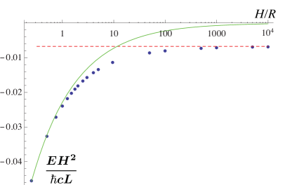
Figure 2: The energy per unit length times $H^{2}$, ${\cal E}H^{2}/(\hbar cL)$, plotted versus $H/R$ for $\theta_{C}=0$ and $R=1$ on a log-linear scale. The dashed line gives the $R=0$ limit and the solid curve gives the PFA result.

It is straightforward to extend this calculation to the case where the parabolic cylinder (of any radius) is rotated by an angle $\theta_{C}$ around its focal axis, as shown in Fig. 3. In place of Eq. (34), we have

$${\cal U}_{\nu k_{x}}(d,\theta_{C})=\frac{1}{\sqrt{\nu!\sqrt{2\pi}}}\frac{\left(\tan\frac{\phi+\theta_{C}}{2}\right)^{\nu}}{\cos\frac{\phi+\theta_{C}}{2}}e^{ik_{y}d}\hbox{\quad and \quad}\hat{\cal U}_{\nu k_{x}}(d,\theta_{C})={\cal U}_{\nu k_{x}}(d,-\theta_{C})\,.$$ (44)

However, now the integral over $k_{x}$ is not symmetric, and the matrix elements with $\nu+\nu^{\prime}$ odd need not vanish.

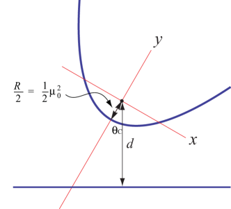
Figure 3: The geometry of a tilted parabolic cylinder in front of a plane.

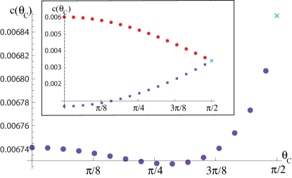
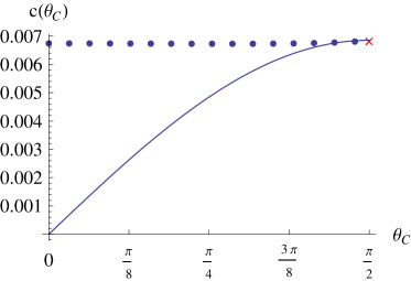
Figure 4: The dependence of the Casimir energy on the tilt angle for a half-plane opposite a plane. The half-plane is a parabolic cylinder with $R=0$, which is oriented perpendicular to the plane for $\theta_{C}=0$ and parallel to the plane for $\theta_{C}=\pi/2$. The left panel shows the coefficient $c(\theta_{C})$ (see text) as a function of $\theta_{C}$, with the exact parallel plate result at $\theta_{C}=\pi/2$ marked with a cross. The inset shows the Dirichlet (circles) and Neumann (squares) contributions to the full electromagnetic result. The right panel again shows $c(\theta_{C})$, but now in comparison to the proximity force approximation (solid line). Note the large discrepancy between the PFA and the exact results as $\theta_{C}\to 0$.

We again consider the $R\to 0$ limit in analyzing this result. From dimensional analysis, the electromagnetic Casimir energy at $R=0$ takes the now $\theta_{C}$-dependent form

$$\frac{{\cal E}}{\hbar cL}=-\frac{C(\theta_{C})}{H^{2}}\,,$$ (45)

where $H=d$ for $R=0$. Following Ref. Gies , which considers the Casimir energy for a scalar field with Dirichlet boundary conditions in this geometry, we plot $c(\theta_{C})=\cos(\theta_{C})C(\theta_{C})$ in Fig. 4. A particularly interesting limit is $\theta_{C}\to\pi/2$, as the two plates become parallel. In this case, the leading contribution to the Casimir energy should be proportional to the area of the half-plane according to the parallel plate formula, ${\cal E}_{\parallel}/(\hbar cA)=-c_{\parallel}/H^{3}$ with $c_{\parallel}=\pi^{2}/720$, plus a subleading correction due to the edge. Multiplying by $\cos\theta_{C}$ has removed the divergence in $C(\theta_{C})$ as $\theta_{C}\to\pi/2$. As in Ref. Gies , we assume $c(\theta_{C}\to\pi/2)=c_{\parallel}/2+\left(\theta_{C}-\pi/2\right)c_{\hbox{\tiny edge}}$, although we cannot rule out the possibility of additional non-analytic forms, such as logarithmic or other singularities. With this assumption, we can estimate the edge correction $c_{\hbox{\tiny edge}}=0.0009$ from the data in Fig. 4. From the inset in Fig. 4, we estimate the Dirichlet and Neumann contributions to this result to be $c_{\hbox{\tiny edge}}^{D}=-0.0025$ (in agreement with Gies within our error estimates) and $c_{\hbox{\tiny edge}}^{N}=0.0034$ respectively. Because higher partial waves become more important as $\theta_{C}\to\pi/2$, reflecting the divergence in $C(\theta_{C})$ in this limit, we have used larger values of $\nu_{\hbox{\tiny max}}$ for $\theta_{C}$ near $\pi/2$. In Fig. 4 we also show a comparison to the proximity force approximation. The PFA is clearly of no use at $\theta_{C}=0$, since it simply gives zero, while at $\theta_{C}=\pi/2$ the PFA gives the correct energy but incorrectly has zero slope, since it misses the edge correction.

We have found that the edge correction is small in the electromagnetic case, as a result of the near-cancellation between the Dirichlet and Neumann contributions. By using Babinet’s principle, it is possible to show that this suppression of edge effects is a general feature of any thin conductor, arising because the leading term in the multiple reflection expansion is identically zero Babinet .

IV Two Parabolic Cylinders

We next consider the force between two parabolic cylinders opening in opposite directions, as shown in the left panel of Fig. 5. We will consider the generalization to arbitrary orientation below. We need to express the outgoing waves from one parabolic cylinder in terms of the regular waves for the other. We let $\bar{\bm{r}}$ represent the coordinates of the second parabolic cylinder, $x=\bar{x}$, $y=-\bar{y}-d$, and $z=\bar{z}$. Using Eq. (32) for $\bar{\bm{r}}$, we have

$$\psi_{\nu}^{\hbox{\tiny out}}(\bar{\bm{r}})=e^{ik_{z}z}\frac{1}{\sqrt{8\pi}}\int_{-\infty}^{\infty}dk_{x}\frac{i}{k_{y}}\frac{\left(\tan\frac{\phi}{2}\right)^{\nu}}{\cos\frac{\phi}{2}}e^{ik_{x}x+ik_{y}y+ik_{y}d}\,.$$ (46)

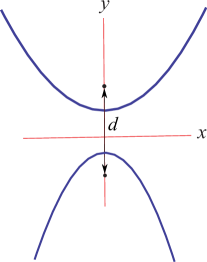
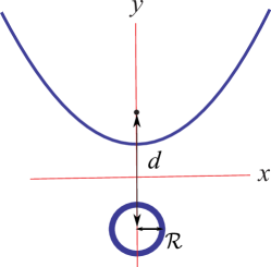
Figure 5: Exterior parabolic cylinder geometries: Two parabolic cylinders outside one another (left panel) and an ordinary cylinder outside a parabolic cylinder (right panel).

Now we use the expansion of the plane wave, Eq. (20), to obtain

$$\psi_{\nu}^{\hbox{\tiny out}}(\bar{\bm{r}})=\sum_{\nu^{\prime}=0}^{\infty}\left[\frac{1}{\nu^{\prime}!\sqrt{8\pi}}\int_{-\infty}^{\infty}dk_{x}\frac{i}{k_{y}}\frac{\left(\tan\frac{\phi}{2}\right)^{\nu+\nu^{\prime}}}{\cos^{2}\frac{\phi}{2}}e^{ik_{y}d}\right]\psi_{\nu^{\prime}}^{\hbox{\tiny reg}}(\bm{r})\,,$$ (47)

where $d$ is the interfocal separation. We can then obtain the translation coefficient from the quantity in brackets. We thus obtain the Casimir interaction energy

$$\frac{\cal E}{\hbar cL}=\int_{0}^{\infty}\frac{d\kappa}{2\pi}\int_{-\infty}^{\infty}\frac{dk_{z}}{2\pi}\log\det\left(\mathbbm{1}_{\nu\nu^{\prime}}-{\cal T}_{\nu}^{C}\sum_{\nu^{\prime\prime}=0}^{\infty}{\cal U}_{\nu\nu^{\prime\prime}}(d){\cal T}_{\nu^{\prime\prime}}^{\bar{C}}\hat{\cal U}_{\nu^{\prime\prime}\nu^{\prime}}(d)\right)\,,$$ (48)

where ${\cal T}^{C}$ and ${\cal T}^{\bar{C}}$ are the scattering $T$-matrix elements for the two parabolic cylinders (which can have different radii), the translation matrix elements are given by

$${\cal U}_{\nu\nu^{\prime}}(d)=\hat{\cal U}_{\nu\nu^{\prime}}(d)=\frac{1}{\sqrt{8\pi\nu!\nu^{\prime}!}}\int_{-\infty}^{\infty}dk_{x}\frac{i}{k_{y}}\frac{\left(\tan\frac{\phi}{2}\right)^{\nu+\nu^{\prime}}}{\cos^{2}\frac{\phi}{2}}e^{ik_{y}d}\,,$$ (49)

and the determinant runs over $\nu,\nu^{\prime}=0,1,2,3,\cdots$. Here again we have defined $\displaystyle\hat{\cal U}_{\nu\nu^{\prime}}(d)=(-1)^{\nu+\nu^{\prime}}{\cal U}_{\nu\nu^{\prime}}(d)^{\dagger}$, where $\displaystyle{\cal U}_{\nu\nu^{\prime}}(d)^{\dagger}$ is the reverse translation matrix. We sum the results for Dirichlet and Neumann boundary conditions to obtain the result for electromagnetism. The analogous numerical simplifications apply here as in the case of the plane, and we can use Eq. (39), now with $d$ instead of $2d$, to express the translation matrix elements in Eq. (49) in terms of the Bateman ${\rm k}$-function. The extension to the tilted case is also analogous; now the angle of rotation can be different for the two translation matrices, corresponding to different angles of rotation for the two parabolic cylinders. We can also introduce a translation in the $x$-direction $d_{x}$, in addition to the existing translation $d$ in the $y$-direction. For rotations $\theta_{C}$ and $\bar{\theta}_{C}$ of the two parabolic cylinders and $x$-translation $d_{x}$, we have

$${\cal U}_{\nu\nu^{\prime}}(d,\theta_{C},\bar{\theta}_{C},d_{x}) = \frac{1}{\sqrt{8\pi\nu!\nu^{\prime}!}}\int_{-\infty}^{\infty}dk_{x}\frac{i}{k_{y}}\frac{\left(\tan\frac{\phi+\theta_{C}}{2}\right)^{\nu}}{\cos\frac{\phi+\theta_{C}}{2}}\frac{\left(\tan\frac{\phi+\bar{\theta}_{C}}{2}\right)^{\nu^{\prime}}}{\cos\frac{\phi+\bar{\theta}_{C}}{2}}e^{ik_{y}d}e^{ik_{x}d_{x}}\,,$$ (50)

$$\hat{\cal U}_{\nu\nu^{\prime}}(d,\theta_{C},\bar{\theta}_{C},d_{x}) = {\cal U}_{\nu\nu^{\prime}}(d,-\theta_{C},-\bar{\theta}_{C},-d_{x})\,,$$ (51)

where we must have $d>0$, but $d_{x}$ can have either sign, representing a translation in either horizontal direction.

By considering two parabolic cylinders of zero radius, we can study the Casimir interactions of two half-planes, as illustrated in Fig. 6. These techniques, together with a multiple reflection expansion, were used in Ref. planes to obtain a variety of results in half-plane geometries.

Figure 6: Two half–planes tilted by angles $\theta_{C}$ and $\overline{\theta}_{C}$, and displaced by $d_{x}$ and $d$.

We take $\theta_{C}=\bar{\theta}_{C}=\pi/2$, so that we are considering parallel half-planes, where positive $d_{x}$ gives the width of the region over which they overlap, while negative $d_{x}$ gives a horizontal displacement of the edges away from each other. In this case, Eq. (51) simplifies to

$${\cal U}_{\nu\nu^{\prime}}\left(d,\frac{\pi}{2},\frac{\pi}{2},d_{x}\right)=\hat{\cal U}_{\nu\nu^{\prime}}\left(d,\frac{\pi}{2},\frac{\pi}{2},d_{x}\right)=\frac{1}{\sqrt{2\pi\nu!\nu^{\prime}!}}\int_{-\infty}^{\infty}dv\frac{(1-iv)^{(\nu+\nu^{\prime}-1)/2}}{(1+iv)^{(\nu+\nu^{\prime}+3)/2}}e^{id_{x}v\sqrt{\kappa^{2}+k_{z}^{2}}}e^{-d\sqrt{v^{2}+1}\sqrt{\kappa^{2}+k_{z}^{2}}}\,.$$ (52)

Results are shown in Fig. 7, along with approximations valid in two limiting cases: First, for $d_{x}$ very negative, we can ignore the vertical displacement. The configuration is then equivalent to the case of $\theta_{C}=\bar{\theta}_{C}=0$, which gives ${\cal E}/(\hbar cL)=-0.0020856/d^{2}$ at separation $d$, which is shown as a dashed line in Fig. 7. Second, for $d_{x}$ large and positive, we can take the standard result for parallel plates ${\cal E}_{\parallel}/(\hbar cL)=-\pi^{2}d_{x}/(720d^{3})$ plus twice the edge correction ${\cal E}_{\hbox{\tiny edge}}/(\hbar cL)=0.0009/d^{2}$ found above for a half-plane parallel to a plane, which is shown as a solid line in Fig. 7.

As these examples illustrate, our description of the two half-planes is redundant: Different parameter choices lead to the same physical configuration, a property we have used to check our calculations. The numerical convergence of physically equivalent configurations can be quite different, however. For example, in the case of $\theta=\bar{\theta}=0$, when both $d_{x}$ and $d$ increase, the Casimir interaction energy decreases, since the half-planes are becoming further apart. In the scattering bases we have chosen, however, in $d$ this effect appears directly through a decaying exponential, while in $d_{x}$ it appears through the cancellation of an oscillating integrand. As a result, we need to maintain $d>0$, but can consider either sign of $d_{x}$.

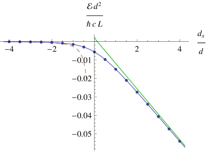
Figure 7: Electromagnetic Casimir interaction energy per unit length for overlapping planes as a function of horizontal displacement, in units of the vertical separation $d$. Solid points are obtained from the exact calculation described in the text. The solid line connecting them is a rational function fit to guide the eye. The dashed line gives the energy for the limit where the planes are edge-to-edge, while the solid straight line gives the standard parallel plate result for the overlap area, plus edge corrections.

V Parabolic Cylinder and Ordinary cylinder

We next consider the case of an ordinary cylinder outside a parabolic cylinder, as shown in the right panel of Fig. 5. In ordinary cylindrical coordinates, we have regular solutions given in terms of Bessel functions, $e^{ik_{z}z}e^{i\ell\theta}J_{\ell}(\sqrt{k^{2}-k_{z}^{2}}r)$, and outgoing solutions given in terms of Hankel functions of the first kind, $e^{ik_{z}z}e^{i\ell\theta}H^{(1)}_{\ell}(\sqrt{k^{2}-k_{z}^{2}}r)$, both indexed by angular momentum $\ell$. We use the expansion of a plane wave in regular ordinary cylindrical wavefunctions,

$$e^{i\bm{k}\cdot\bm{r}}=e^{ik_{z}z}\sum_{\ell=-\infty}^{\infty}e^{i\ell\phi}e^{i\ell\theta}J_{\ell}(\sqrt{k^{2}-k_{z}^{2}}r)\,,$$ (53)

where $\phi$ is defined as in Eq. (21) and $\theta$ and $r$ are the ordinary cylindrical coordinates for $\bm{r}$. In these coordinates, the free Green’s function is given by

$$G(\bm{r}_{1},\bm{r}_{2},k)=\frac{i}{4}\int_{-\infty}^{\infty}\frac{dk_{z}}{2\pi}e^{ik_{z}(z_{1}-z_{2})}\sum_{\ell=-\infty}^{\infty}e^{i\ell(\theta_{1}-\theta_{2})}J_{\ell}(\sqrt{k^{2}-k_{z}^{2}}r_{<})H^{(1)}_{\ell}(\sqrt{k^{2}-k_{z}^{2}}r_{>})\,,$$ (54)

where $r_{<}$ ($r_{>}$) is the smaller (larger) of $r_{1}$ and $r_{2}$.

The $T$-matrix elements for an ordinary cylinder of radius ${\cal R}$ are given in terms of Bessel and Hankel functions and their modified counterparts by $\displaystyle{\cal T}_{\ell k_{z}\ell^{\prime}k_{z}^{\prime}}=2\pi\delta(k_{z}-k_{z}^{\prime})\delta_{\ell\ell^{\prime}}{\cal T}_{\ell}^{O}$, with

$${\cal T}_{\ell}^{O} = -\frac{J_{\ell}\left({\cal R}\sqrt{k^{2}-k_{z}^{2}}\right)}{H_{\ell}^{(1)}\left({\cal R}\sqrt{k^{2}-k_{z}^{2}}\right)}=-\frac{\pi}{2}i^{2\ell+1}\frac{I_{\ell}\left({\cal R}\sqrt{\kappa^{2}+k_{z}^{2}}\right)}{K_{\ell}\left({\cal R}\sqrt{\kappa^{2}+k_{z}^{2}}\right)}\hbox{\qquad(Dirichlet),}$$ (55)

$${\cal T}_{\ell}^{O} = -\frac{J_{\ell}^{\prime}\left({\cal R}\sqrt{k^{2}-k_{z}^{2}}\right)}{H_{\ell}^{(1)}{}^{\prime}\left({\cal R}\sqrt{k^{2}-k_{z}^{2}}\right)}=-\frac{\pi}{2}i^{2\ell+1}\frac{I_{\ell}^{\prime}\left({\cal R}\sqrt{\kappa^{2}+k_{z}^{2}}\right)}{K_{\ell}^{\prime}\left({\cal R}\sqrt{\kappa^{2}+k_{z}^{2}}\right)}\hbox{\quad(Neumann),}$$ (56)

where prime indicates a derivative with respect to the function’s argument.

For an ordinary cylinder outside a parabolic cylinder with separation $d$ between the center of the ordinary cylinder and the focus of the parabolic cylinder, we substitute Eq. (53) into Eq. (46) to obtain

$$\psi_{\nu}^{\hbox{\tiny out}}(\bar{\bm{r}}) = e^{ik_{z}z}\frac{1}{\sqrt{8\pi}}\int_{-\infty}^{\infty}dk_{x}\frac{i}{k_{y}}\frac{\left(\tan\frac{\phi}{2}\right)^{\nu}}{\cos\frac{\phi}{2}}e^{ik_{y}d}\sum_{\ell=-\infty}^{\infty}e^{i\ell\phi}e^{i\ell\theta}J_{\ell}(\sqrt{k^{2}-k_{z}^{2}}r)$$ (57)

$$= \sum_{\ell=-\infty}^{\infty}\left[\frac{1}{\sqrt{8\pi}}\int_{-\infty}^{\infty}dk_{x}\frac{i}{k_{y}}e^{i\ell\phi}\frac{\left(\tan\frac{\phi}{2}\right)^{\nu}}{\cos\frac{\phi}{2}}e^{ik_{y}d}\right]e^{ik_{z}z}e^{i\ell\theta}J_{\ell}(\sqrt{k^{2}-k_{z}^{2}}r)\,,$$ (58)

where again the quantity in brackets is the coefficient we need to compute the translation matrix.

We thus obtain the Casimir interaction energy

$$\frac{\cal E}{\hbar cL}=\int_{0}^{\infty}\frac{d\kappa}{2\pi}\int_{-\infty}^{\infty}\frac{dk_{z}}{2\pi}\log\det\left(\mathbbm{1}_{\nu\nu^{\prime}}-{\cal T}_{\nu}^{C}\sum_{\ell=-\infty}^{\infty}{\cal U}_{\nu\ell}(d){\cal T}_{\ell}^{O}\hat{\cal U}_{\nu^{\prime}\ell}(d)\right)\,,$$ (59)

where

$${\cal U}_{\nu\ell}(d)=\hat{\cal U}_{\nu\ell}(d)=\frac{1}{\sqrt{\nu!\sqrt{2\pi}}}\sqrt{\frac{4(-1)^{\ell}}{i}}\frac{1}{\sqrt{8\pi}}\int_{-\infty}^{\infty}dk_{x}\frac{i}{k_{y}}e^{i\ell\phi}\frac{\left(\tan\frac{\phi}{2}\right)^{\nu}}{\cos\frac{\phi}{2}}e^{ik_{y}d}$$ (60)

and the determinant again runs over $\nu,\nu^{\prime}=0,1,2,3,\cdots$. As before, for convenience we have defined $\displaystyle\hat{\cal U}_{\nu\ell}(d)=(-1)^{\nu+\ell}{\cal U}_{\nu\ell}(d)^{\dagger}$, where $\displaystyle{\cal U}_{\nu\ell}(d)^{\dagger}$ is the reverse translation matrix. We can again simplify this expression for numerical computation by combining the $\kappa$ and $k_{z}$ integrals, and by exploiting symmetries in $\ell\to-\ell$ and $k_{x}\to-k_{x}$. Generalizations to include horizontal translation and tilt of the parabolic cylinder also work in the same way as before, and taking the limit in which the radius of the parabolic cylinder goes to zero gives the Casimir energy for a cylindrical wire opposite a half-plane.

VI Interior Geometries

Up to now, we have considered “exterior” geometries in which the objects are outside one another. However, simple modifications of these techniques enable us to also consider “interior” geometries using the formalism of Ref. interior . (Interior geometries were also considered in Lombardo , using large-scale computation.) There are two changes required for this case: The $T$-matrix of the outside object must be inverted, and we require the translation matrix connecting the regular solutions for the different objects, rather than the one connecting outgoing solutions for one object to regular solutions for the other.

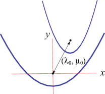
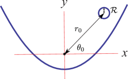
Figure 8: Interior parabolic cylinder geometries: Two parabolic cylinders inside one another (left panel) and an ordinary cylinder inside a parabolic cylinder (right panel).

We first consider two parabolic cylinders inside one another. We parameterize the displacement between their foci in parabolic cylinder coordinates by $\lambda_{0}$ and $\mu_{0}$, as shown in the left panel of Fig. 8. Following Ref. Epstein , we can derive the translation matrix for regular solutions appropriate to the inside problem. Let $\bm{r}^{\prime}=\bm{r}+\bm{r}_{0}$ and consider the equation $e^{i\bm{k}\cdot\bm{r}^{\prime}}=e^{i\bm{k}\cdot\bm{r}_{0}}e^{i\bm{k}\cdot\bm{r}}$. Using Eq. (20), we have

$$\frac{1}{\cos\frac{\phi}{2}}\sum_{\nu^{\prime}=0}^{\infty}\frac{1}{\nu^{\prime}!}\left(\tan\frac{\phi}{2}\right)^{\nu^{\prime}}\psi_{\nu^{\prime}}^{\hbox{\tiny reg}}(\lambda^{\prime},\mu^{\prime}) = \frac{1}{\cos\frac{\phi}{2}}\sum_{\nu_{0}=0}^{\infty}\frac{1}{\nu_{0}!}\left(\tan\frac{\phi}{2}\right)^{\nu_{0}}\psi_{\nu_{0}}^{\hbox{\tiny reg}}(\lambda_{0},\mu_{0})$$ (61)

$$\times \frac{1}{\cos\frac{\phi}{2}}\sum_{\nu=0}^{\infty}\frac{1}{\nu!}\left(\tan\frac{\phi}{2}\right)^{\nu}\psi_{\nu}^{\hbox{\tiny reg}}(\lambda,\mu)\,.$$ (62)

Now we let $\displaystyle t=\tan\frac{\phi}{2}$, so $\displaystyle\cos\frac{\phi}{2}=\frac{1}{\sqrt{1+t^{2}}}$, and consider the case where $|t|<1$ to obtain

$$\sum_{\nu^{\prime}=0}^{\infty}\frac{t^{\nu^{\prime}}}{\nu^{\prime}!}\psi_{\nu^{\prime}}^{\hbox{\tiny reg}}(\lambda^{\prime},\mu^{\prime})=\sqrt{1+t^{2}}\sum_{\nu_{0}=0}^{\infty}\frac{t^{\nu_{0}}}{\nu_{0}!}\psi_{\nu_{0}}^{\hbox{\tiny reg}}(\lambda_{0},\mu_{0})\sum_{\nu=0}^{\infty}\frac{t^{\nu}}{\nu!}\psi_{\nu}^{\hbox{\tiny reg}}(\lambda,\mu)\,.$$ (63)

Next we write

$$\sqrt{1+t^{2}}=\sum_{n=0}^{\infty}\alpha_{n}t^{n}\,,\hbox{\quad where \quad}\alpha_{n}=\left\{\begin{array}[]{l@{\quad}l}0&\hbox{if $n$ is odd}\cr\frac{(-1)^{n/2}\Gamma\left(\frac{n-1}{2}\right)}{\Gamma\left(-\frac{1}{2}\right)\frac{n}{2}!}&\hbox{if $n$ is even}\end{array}\right.\,.$$ (64)

Substituting this result into Eq. (63) and equating powers of $t$ results in

$$\psi_{\nu^{\prime}}^{\hbox{\tiny reg}}(\lambda^{\prime},\mu^{\prime})=\sum_{\nu=0}^{\nu^{\prime}}\left[\sum_{\nu_{0}=0}^{\nu^{\prime}-\nu}\frac{\nu^{\prime}!}{\nu!\nu_{0}!}\alpha_{\nu^{\prime}-\nu-\nu_{0}}\psi_{\nu_{0}}^{\hbox{\tiny reg}}(\lambda_{0},\mu_{0})\right]\psi_{\nu}^{\hbox{\tiny reg}}(\lambda,\mu)\,,$$ (65)

which yields the coefficient we need from the quantity in brackets.

The Casimir interaction energy is then

$$\frac{\cal E}{\hbar cL}=\int_{0}^{\infty}\frac{d\kappa}{2\pi}\int_{-\infty}^{\infty}\frac{dk_{z}}{2\pi}\log\det\left(\mathbbm{1}_{\nu\nu^{\prime}}-\left({\cal T}_{\nu}^{C}\right)^{-1}{\cal V}_{\nu\nu^{\prime}}(\lambda_{0},\mu_{0}){\cal T}_{\nu^{\prime}}^{\bar{C}}\hat{\cal V}_{\nu\nu^{\prime}}(\lambda_{0},\mu_{0})\right)\,,$$ (66)

where ${\cal T}_{\nu}^{C}$ (${\cal T}_{\nu}^{\bar{C}}$) is the $T$-matrix for the outer (inner) parabolic cylinder,

$${\cal V}_{\nu\nu^{\prime}}(\lambda_{0},\mu_{0})=\hat{\cal V}_{\nu\nu^{\prime}}(-\lambda_{0},\mu_{0})=\sum_{\nu_{0}=0}^{\nu^{\prime}-\nu}\frac{1}{\nu_{0}!}\alpha_{\nu^{\prime}-\nu-\nu_{0}}\psi_{\nu_{0}}^{\hbox{\tiny reg}}(\lambda_{0},\mu_{0})\,,$$ (67)

and we have dropped normalization factors that cancel in the determinant.

For an ordinary cylinder inside a parabolic cylinder, as shown in the right panel of Fig. 8, we again let $\bm{r}^{\prime}=\bm{r}+\bm{r}_{0}$ and consider the equation $e^{i\bm{k}\cdot\bm{r}^{\prime}}=e^{i\bm{k}\cdot\bm{r}_{0}}e^{i\bm{k}\cdot\bm{r}}$, but now we expand the left-hand side in parabolic cylinder coordinates and the right-hand side in ordinary cylindrical coordinates, to obtain

$$\frac{1}{\cos\frac{\phi}{2}}\sum_{\nu^{\prime}=0}^{\infty}\frac{\left(\tan\frac{\phi}{2}\right)^{\nu^{\prime}}}{\nu^{\prime}!}\psi_{\nu^{\prime}}^{\hbox{\tiny reg}}(\lambda^{\prime},\mu^{\prime})=e^{ik_{z}z_{0}}\sum_{\ell_{0}=-\infty}^{\infty}e^{i\ell_{0}\phi}e^{i\ell_{0}\theta_{0}}J_{\ell_{0}}(\sqrt{k^{2}-k_{z}^{2}}r_{0})e^{ik_{z}z}\sum_{\ell=-\infty}^{\infty}e^{i\ell\phi}e^{i\ell\theta}J_{\ell}(\sqrt{k^{2}-k_{z}^{2}}r)\,.$$ (68)

As before, setting $\displaystyle t=\tan\frac{\phi}{2}$, so that $\displaystyle\sqrt{1+t^{2}}=\frac{1}{\cos\frac{\phi}{2}}$ and $\displaystyle\phi=\frac{1}{i}\log\frac{1+it}{1-it}$, yields

$$\sum_{\nu^{\prime}=0}^{\infty}\frac{t^{\nu^{\prime}}}{\nu^{\prime}!}\psi_{\nu^{\prime}}^{\hbox{\tiny reg}}(\lambda^{\prime},\mu^{\prime})=\frac{1}{\sqrt{1+t^{2}}}\sum_{\ell=-\infty}^{\infty}\sum_{\ell_{0}=-\infty}^{\infty}\left(\frac{1+it}{1-it}\right)^{\ell+\ell_{0}}e^{ik_{z}z_{0}}e^{i\ell_{0}\theta_{0}}J_{\ell_{0}}(\sqrt{k^{2}-k_{z}^{2}}r_{0})e^{ik_{z}z}e^{i\ell\theta}J_{\ell}(\sqrt{k^{2}-k_{z}^{2}}r)\,.$$ (69)

We take $\nu$ derivatives with respect to $t$ and then set $t=0$ to obtain

$$\psi_{\nu}^{\hbox{\tiny reg}}(\lambda^{\prime},\mu^{\prime})=\sum_{\ell=-\infty}^{\infty}\left[\sum_{\ell_{0}=-\infty}^{\infty}\frac{d^{\nu}}{dt^{\nu}}\left(\frac{1}{\sqrt{1+t^{2}}}\left(\frac{1+it}{1-it}\right)^{\ell+\ell_{0}}\right|_{t=0}e^{ik_{z}z_{0}}e^{i\ell_{0}\theta_{0}}J_{\ell_{0}}(\sqrt{k^{2}-k_{z}^{2}}r_{0})\right]e^{ik_{z}z}e^{i\ell\theta}J_{\ell}(\sqrt{k^{2}-k_{z}^{2}}r)\,,$$ (70)

where again the quantity in brackets will give the coefficient we need. Using the generalized binomial expansion, we obtain

$$\beta_{\nu,\ell}=\frac{d^{\nu}}{dt^{\nu}}\left(\frac{1}{\sqrt{1+t^{2}}}\left(\frac{1+it}{1-it}\right)^{\ell}\right|_{t=0}=\nu!\sum_{\genfrac{}{}{0.0pt}{1}{n=0}{n\equiv\,\nu\bmod 2}}^{\min(2|\ell|,\nu)}\frac{(2|\ell|)!}{n!(2|\ell|-n)!}(\pm i)^{n}\frac{\Gamma\left(\frac{1}{2}-|\ell|\right)}{\left(\frac{\nu-n}{2}\right)!\,\Gamma\left(\frac{1}{2}-|\ell|+\frac{n-\nu}{2}\right)}\,,$$ (71)

where the $\pm$ is $+$ for $\ell\geq 0$ and $-$ for $\ell<0$, and the sum starts at $n=0$ for $\nu$ even and $n=1$ for $\nu$ odd, and then in both cases goes in steps of $2$. For a configuration where the displacement from the focus of the parabolic cylinder to the center of the ordinary cylinder is parameterized in ordinary cylindrical coordinates by distance $r_{0}$ and angle $\theta_{0}$ from the $x$-axis, the Casimir interaction energy is then

$$\frac{\cal E}{\hbar cL}=\int_{0}^{\infty}\frac{d\kappa}{2\pi}\int_{-\infty}^{\infty}\frac{dk_{z}}{2\pi}\log\det\left(\mathbbm{1}_{\nu\nu^{\prime}}-\left({\cal T}_{\nu}^{C}\right)^{-1}\sum_{\ell=-\infty}^{\infty}{\cal V}_{\nu\ell}(r_{0},\theta_{0}){\cal T}_{\ell}^{O}\hat{\cal V}_{\nu^{\prime}\ell}(r_{0},\theta_{0})\right)\,,$$ (72)

where ${\cal T}_{\nu}^{C}$ is the $T$-matrix for the (outer) parabolic cylinder, ${\cal T}_{\ell}^{O}$ is the $T$-matrix for the (inner) ordinary cylinder, and

$${\cal V}_{\nu\ell}(r_{0},\theta_{0})=\hat{\cal V}_{\nu\ell}(r_{0},\pi-\theta_{0})=\frac{1}{\sqrt{\nu!\sqrt{2\pi}}}\sqrt{\frac{4(-1)^{\ell}}{i}}\left[\sum_{\ell_{0}=-\infty}^{\infty}\beta_{\nu,\ell+\ell_{0}}e^{i\ell_{0}\theta_{0}}i^{\ell_{0}}I_{\ell_{0}}(\sqrt{\kappa^{2}+k_{z}^{2}}r_{0})\right]\,.$$ (73)

As an example, we consider a thin wire near the focal axis of a parabolic cylinder with parabolic radius $\mu_{0}^{2}$. To leading order in the needle radius ${\cal R}$, we only need the $\ell=0$ Dirichlet $T$-matrix element, which goes like $1/\log{\cal R}$ for ${\cal R}$ small. Keeping only the leading term in $1/\log({\cal R}/\mu_{0}^{2})$ and also expanding in the displacement from the focus $r_{0}$, we obtain

$$\frac{\cal E}{\hbar cL}\approx\frac{3}{32\mu_{0}^{4}\log\frac{{\cal R}}{\mu_{0}^{2}}}-\frac{5}{16\mu_{0}^{6}\log\frac{{\cal R}}{\mu_{0}^{2}}}r_{0}\sin\theta_{0}+\frac{15}{256\mu_{0}^{8}\log\frac{\cal R}{\mu_{0}^{2}}}r_{0}^{2}(9-5\cos 2\theta_{0})+\cdots\,.$$ (74)

Here energy is calculated in comparison to the configuration where the ordinary cylinder is placed at $x=0$, $y=\infty$. In deriving this result, we have assumed that ${\cal R}\ll\mu_{0}^{2}$ is small enough that we can drop terms proportional to $\log(\mu_{0}^{2}\sqrt{\kappa^{2}+k_{z}^{2}})$ in comparison to terms proportional to $\log({\cal R}/\mu_{0}^{2})$, since for $\sqrt{\kappa^{2}+k_{z}^{2}}\gg 1/\mu_{0}^{2}$ the integrand in Eq. (72) is exponentially suppressed. The first term gives the (negative) Casimir interaction energy per unit length when the wire is at the focus, while the second and third terms give the correction as it is moved a small distance away. The angular dependence is exactly as we would expect: as the wire moves closer to the vertex axis of the parabolic cylinder ($\theta_{0}=-\pi/2$), the energy gets more negative; as it moves away from the vertex axis ($\theta_{0}=\pi/2$) the energy is less negative, and if it moves in a direction perpendicular to the plane of symmetry of the parabolic cylinder ($\theta_{0}=0$ or $\theta_{0}=\pi$), the energy is unchanged to first order. As a result, unlike the geometric optics calculation considered in Ref. Ford , here we do not see any unusual behavior of the Casimir energy at the focus, which is in agreement with the results in Ref. Lombardo . In Fig. 9 we illustrate this result for the case where the radius of the ordinary cylinder and its displacement are not small. We choose the same radii for the parabolic and ordinary cylinders as in Ref. Lombardo , and the results we obtain are approximately in agreement with what was found there. We cannot make a precise comparison, however, because in that work the parabolic cylinder is of finite size and closed at the far end.

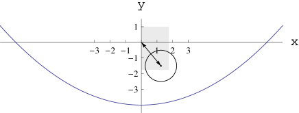
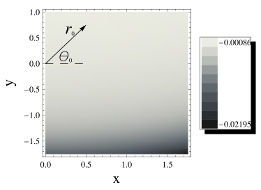
Figure 9: Casimir interaction energy for an ordinary cylinder inside a parabolic cylinder. The left panel shows the geometry, with the focus of the parabolic cylinder placed at the origin. We choose the same radii as Ref. Lombardo , $\mu_{0}=\sqrt{8}$ and ${\cal R}=1$, so that the vertex line of the parabolic cylinder lies at $x=0$, $y=-4$. The right panel shows the Casimir interaction energy per unit length ${\cal E}/(\hbar cL)$ as a function of $x$ and $y$, the displacement of the center of the ordinary cylinder from the focus of the parabolic cylinder, where the center of the ordinary cylinder lies within the shaded region of the left panel.

VII Nonzero Temperature

It is straightforward to extend all of these results to temperature $T\neq 0$, a subject that has been of significant recent interest Weber . In each calculation, we simply replace the integral $\int_{0}^{\infty}\frac{d\kappa}{2\pi}$ by the sum $\frac{Tk_{B}}{\hbar c}{\sum_{n=0}^{\infty}}^{\prime}$ over Matsubara frequencies $\kappa_{n}=2\pi nk_{B}T/(\hbar c)$, where $k_{B}$ is Boltzmann’s constant and the prime indicates that the $n=0$ mode is counted with a weight of $1/2$ universal . In the classical limit of asymptotically large temperature, only the $n=0$ term contributes. The numerical calculation is more cumbersome for $T\neq 0$, because for $T=0$ we could always make the substitution $\displaystyle\int_{0}^{\infty}\frac{d\kappa}{2\pi}\int_{-\infty}^{\infty}\frac{dk_{z}}{2\pi}f(\sqrt{\kappa^{2}+k_{z}^{2}})\to\frac{1}{4\pi}\int_{0}^{\infty}qdqf(q)$, where $q=\sqrt{\kappa^{2}+k_{z}^{2}}$, since the quantity we integrate depends only on $q$. We find it convenient to continue to use the integration variable $q$, since the quantity we now sum and integrate still depends only on this quantity. We therefore carry out the sum and integral via the replacement

$$\frac{k_{B}T}{\hbar c}{\sum_{n=0}^{\infty}}^{\prime}\int_{-\infty}^{\infty}\frac{dk_{z}}{2\pi}f(\sqrt{\kappa_{n}^{2}+k_{z}^{2}})\to\frac{k_{B}T}{\hbar c}\left[\int_{0}^{\infty}\frac{dk_{z}}{2\pi}f(k_{z})+\int_{0}^{\infty}\frac{dq}{\pi}\sum_{n=1}^{\lfloor\frac{\hbar cq}{2\pi k_{B}T}\rfloor}\frac{q}{\sqrt{q^{2}-\kappa_{n}^{2}}}f(q)\right]\,,$$ (75)

where $\lfloor x\rfloor$ denotes the greatest integer less than or equal to $x$.

As an example, we consider thermal corrections for a conducting half-plane (a parabolic cylinder with $R=0$) oriented perpendicular to a conducting plane, at separation $H$. In the classical limit, only the $n=0$ mode contributes and we obtain the energy ${\cal E}/L=-k_{B}TC_{T=\infty}/H$, with $C_{T=\infty}=0.0472$. The Dirichlet contribution to this result is $C_{T=\infty}^{D}=0.0394$, in agreement with Ref. Gies . In Fig. 10 the energy for this geometry is shown as a function of temperature. For typical separation distances at room temperature, the thermal corrections are small.

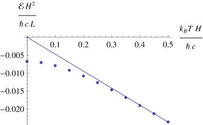
Figure 10: The energy per unit length times $H^{2}$, ${\cal E}H^{2}/(\hbar cL)$, plotted versus $k_{B}TH/(\hbar c)$ for $\theta_{C}=0$ and $R=0$. The solid line gives the $T\to\infty$ limit determined from the lowest Matsubara frequency. For reference, at a separation of $H=350\ {\rm nm}$, a temperature $T=300\ {\rm K}$ corresponds to $k_{B}TH/(\hbar c)\approx 0.046$.

VIII Conclusions

There are only a limited set of coordinate systems in which the vector Helmholtz equation for electromagnetism can be solved exactly. Taking advantage of one of these few cases, we have obtained complete scattering amplitudes for a perfectly conducting parabolic cylinder and employed these results to compute Casimir forces. In principle, Casimir forces can be computed in configurations involving parabolic cylinders and other shapes for which scattering amplitudes are known, as long as we can obtain the translation matrices, which convert expressions of electromagnetic waves between different coordinate basis, appropriate to the individual shapes. Following this procedure, we have computed Casimir forces between a parabolic cylinder, a plane, an ordinary cylinder, and a second parabolic cylinder. The formalism is versatile enough to treat situations in which one object is enclosed in the interior of a parabolic cylinder, and is also easily extended to finite temperatures.

We focus special attention to the limit when the radius of the parabolic cylinder goes to zero, and it evolves into a semi-infinite plate — a knife edge. In this limit we can quantify the contribution of edges to the Casimir force. By examining tilted plates, we can consider a broad range of cases involving interacting edges which should be useful to the design of microelectromechanical devices. Until recently, the state of art computation of Casimir forces relied upon the PFA, which is demonstrably unreliable for a knife edge: A thin metal disk perpendicular to a nearby metal surface experiences a Casimir force described by an extension of Eq. (43), while as indicated in Fig. 2, the PFA approximation to the energy vanishes as the thickness goes to zero. Based on the full result for perpendicular planes, however, we can formulate an “edge PFA,” which yields the energy by integrating $d\mathcal{E}/dL$ from Eq. (43) along the edge of the disk. Letting $r$ be the disk radius, in this approximation we obtain

$$\mathcal{E}_{\hbox{\tiny Epfa}}=-\hbar cC_{\perp}\int_{-r}^{r}(H+r-\sqrt{r^{2}-x^{2}})^{-2}dx\xrightarrow{H/r\to 0}-\hbar cC_{\perp}\pi\sqrt{r/(2H^{3})}\,,$$ (76)

which is valid if the thickness of the disk is small compared to its separation from the plane. (For comparison, note that the ordinary PFA for a metal sphere of radius $r$ and a plate is proportional to $r/H^{2}$.)

A disk may be more experimentally tractable than a plane, since its edge does not need to be maintained parallel to the plate. One possibility is a metal film, evaporated onto a substrate that either has low permittivity or can be etched away beneath the edge of the deposited film. Micromechanical torsion oscillators, which have already been used for Casimir experiments Decca07 , seem readily adaptable for testing Eq. (45). Because the overall strength of the Casimir effect is weaker for a disk than for a sphere, observing Casimir forces in this geometry will require greater sensitivities or shorter separation distances than the sphere-plane case. As the separation gets smaller, however, the dominant contributions arise from higher-frequency fluctuations, and deviations from the perfect conductor limit can become important. While the effects of finite conductivity could be captured by an extension of our method, the calculation becomes significantly more difficult in this case because the matrix of scattering amplitudes is no longer diagonal.

To estimate the range of important frequencies, we consider $R\ll H$ and $\theta_{C}=0$. In this case, the integrand in Eq. (43) is strongly peaked around $q\approx 0.3/H$. As a result, by including only values of $q$ up to $2/H$, we still capture $95\%$ of the full result (and by going up to $3/H$ we include 99%). This truncation corresponds to a minimum “fluctuation wavelength” $\lambda_{\hbox{\tiny min}}=\pi H$. For the perfect conductor approximation to hold, $\lambda_{\hbox{\tiny min}}$ must be large compared to the metal’s plasma wavelength $\lambda_{p}$, so that these fluctuations are well described by assuming perfect reflectivity. We also need the thickness of the disk to be small enough compared to $H$ that the deviation from the proximity force calculation is evident (see Fig. 2), but large enough compared to the metal’s skin depth $\delta$ that the perfect conductor approximation is valid. For a typical metal film, $\lambda_{p}\approx 130\ {\rm nm}$ and $\delta\approx 25\ {\rm nm}$ at the relevant wavelengths. For a disk of radius $r=100\ \mu{\rm m}$, the present experimental frontier of $0.1\ {\rm pN}$ sensitivity corresponds to a separation distance $H\approx 350\ {\rm nm}$, which then falls within the expected range of validity of our calculation according to these criteria. The force could also be enhanced by connecting several identical but well-separated disks. In that case, the same force could be measured at a larger separation distance, where our calculation is more accurate. In the case of overlapping planes, the correction to the traditional PFA energy is of a similar magnitude to the total force for perpendicular planes in the above example, and thus should also be measurable at these separations. We have shown that thermal corrections are generally small at room temperature for typical separations, and furthermore our methods allow these corrections to be computed precisely.

IX Acknowledgments

We thank U. Mohideen for helpful discussions and F. Khoshnoud for correspondence regarding the example of overlapping planes. This work was supported in part by the National Science Foundation (NSF) through grants PHY08-55426 (NG), DMR-08-03315 (SJR and MK), Defense Advanced Research Projects Agency (DARPA) contract No. S-000354 (SJR, MK, and TE), and by the U. S. Department of Energy (DOE) under cooperative research agreement #DF-FC02-94ER40818 (RLJ).

References

(1)
H. B. G. Casimir, Proc. K. Ned. Akad. Wet. 51, 793 (1948).
(2)
S. K. Lamoreaux, Phys. Rev. Lett. 78, 5 (1997);
U. Mohideen and A. Roy,
Phys. Rev. Lett. 81, 4549 (1998);
G. Bressi, G. Carugno, R. Onofrio, and G. Ruoso,
Phys. Rev. Lett. 88, 041804 (2002);
H. B. Chan, V. A. Aksyuk, R. N. Kleiman, D. J. Bishop, and
F. Capasso, Science 291, 1941 (2001).
(3)
F. Capasso, J. N. Munday, D. Iannuzzi and H. B. Chan,
IEEE J. Sel. Top. Quant. 13, 400 (2007).
(4)
M. T. Homer Reid, A. W. Rodriguez, J. White, and S. G. Johnson,
Phys. Rev. Lett. 103, 040401 (2009).
(5)
H. Gies, K. Langfeld and L. Moyaerts,
JHEP 0306, 018 (2003);
H. Gies and K. Klingmüller, Phys. Rev. D
74, 045002 (2006); H. Gies and K. Klingmüller, Phys. Rev. Lett.
97, 220405 (2006).
(6)
S. Pasquali and A. C. Maggs,
Phys. Rev. A 79, 020102 (2009).
(7)
T. Emig, N. Graham, R. L. Jaffe, and M. Kardar,
Phys. Rev. Lett. 99, 170403 (2007);
Phys. Rev. D 77, 025005 (2008).
(8)
S. J. Rahi, T. Emig, N. Graham, R. L. Jaffe and M. Kardar,
Phys. Rev. D 80, 085021 (2009).
(9)
T. Emig, A. Hanke, R. Golestanian, and M. Kardar,
Phys. Rev. Lett. 87, 260402 (2001).
(10)
O. Kenneth and I. Klich,
Phys. Rev. Lett. 97, 160401 (2006).
(11)
R. Balian and B. Duplantier,
Ann. Phys. 104, 300 (1977); 112, 165 (1978).
(12)
J. Schwinger, Lett. Math. Phys. 1, 43 (1975).
(13)
T. Emig, J. Stat. Mech. P04007 (2008).
(14)
S. J. Rahi, T. Emig, R. L. Jaffe, and M. Kardar,
Phys. Rev. A 78, 012104 (2008).
(15)
S. J. Rahi, A. W. Rodriguez, T. Emig, R. L. Jaffe, S. G. Johnson,
and M. Kardar, Phys. Rev. A 77, 030101(R) (2008).
(16)
M. F. Maghrebi, Phys. Rev. D 83, 045004 (2011).
(17)
O. Kenneth, and I. Klich,
Phys. Rev. B 78, 014103 (2008).
(18)
K. A. Milton and J. Wagner,
J. Phys. A 41, 155402 (2008).
(19)
R. Golestanian, Phys. Rev. A 80, 012519 (2009).
(20)
C. Ccapa Ttira, C. D. Fosco and E. L. Losada,
J. Phys. A 43, 235402 (2010).
(21)
N. Graham, A. Shpunt, T. Emig, S. J. Rahi, R. L. Jaffe and M. Kardar,
Phys. Rev. D 81, 061701(R) (2010).
(22)
M. F. Maghrebi, S. J. Rahi, T. Emig, N. Graham,
R. L. Jaffe, and M. Kardar, arXiv:1010.3223.
(23)
H. Gies and K. Klingmuller,
Phys. Rev. Lett. 97, 220405 (2006);
A. Weber and H. Gies,
Phys. Rev. D 80, 065033 (2009).
(24)
D. Kabat, D. Karabali, and V. P. Nair,
Phys. Rev. D 81, 125013 (2010);
Phys. Rev. D 82, 025014 (2010).
(25)
P. Morse and H. Feshbach, Methods of Mathematical Physics
(McGraw-Hill, 1953).
(26)
E. T. Whittaker and G. N. Watson, Modern Analysis
(Cambridge University Press, 1927).
(27)
H. Bateman, Trans. Amer. Math. Soc. 33, 817 (1931).
(28)
E. H. Newman, IEEE Trans. Ant. Prop. 38 (1990) 541.
(29)
M. F. Maghrebi, R. Abravanel, and R. L. Jaffe, arXiv:1103.5395.
(30)
M. F. Maghrebi and N. Graham, arXiv:1102.1486.
(31)
S. Zaheer, S. J. Rahi, T. Emig, and R. L. Jaffe,
Phys. Rev. A 81, 030502(R) (2010).
(32)
F. C. Lombardo, F. D. Mazzitelli, M. Vazquez and P. I. Villar,
Phys. Rev. D 80, 065018 (2009).
(33)
D. Epstein, “On the Functions of the Parabolic Cylinder,”
New York University Institue of Mathematical Sciences, Division of
Electromagnetic Research, Report No. BR-19.
(34)
L. H. Ford and N. F. Svaiter,
Phys. Rev. A 62, 062105 (2000);
Phys. Rev. A 66, 062106 (2002).
(35)
A. Weber and H. Gies,
Phys. Rev. Lett. 105, 040403 (2010);
A. Weber and H. Gies,
Phys. Rev. D 82, 125019 (2010).
(36)
R. S. Decca, D. López, E. Fischbach, G. L. Klimchitskaya,
D. E. Krause, and V. M. Mostepanenko,
Phys. Rev. D 75, 077101 (2007).