Bohr Hamiltonian with deformation-dependent mass term for the Davidson potential

Abstract

Analytical expressions for spectra and wave functions are derived for a Bohr Hamiltonian, describing the collective motion of deformed nuclei, in which the mass is allowed to depend on the nuclear deformation. Solutions are obtained for separable potentials consisting of a Davidson potential in the $\beta$ variable, in the cases of $\gamma$-unstable nuclei, axially symmetric prolate deformed nuclei, and triaxial nuclei, implementing the usual approximations in each case. The solution, called the Deformation Dependent Mass (DDM) Davidson model, is achieved by using techniques of supersymmetric quantum mechanics (SUSYQM), involving a deformed shape invariance condition. Spectra and $B(E2)$ transition rates are compared to experimental data. The dependence of the mass on the deformation, dictated by SUSYQM for the potential used, reduces the rate of increase of the moment of inertia with deformation, removing a main drawback of the model.

I Introduction

The Bohr Hamiltonian Bohr and its extensions, the geometrical collective model BM ; EG , have provided for several decades a sound framework for understanding the collective behaviour of atomic nuclei. It has been customary to consider in the Bohr Hamiltonian the mass to be a constant. However, evidence has been accumulating that this approximation might be inadequate. In particular:

1) The moments of inertia are predicted to increase proportionally to $\beta^{2}$, where $\beta$ is the collective variable corresponding to nuclear deformation, while the experimentally determined (from the spectra) moment of inertia shows a much more moderate increase as a function of the experimentally determined (from the $B(E2)$ transition rates) deformation, especially for well deformed nuclei Ring . This discrepancy has led to arguments that the use of the Bohr Hamiltonian is justified for vibrational and transitional nuclei, but its applicability to deformed nuclei needs further clarification.

2) Detailed comparisons to experimental data have recently pointed out Jolos1 ; Jolos2 that the mass tensor of the collective Hamiltonian cannot be considered as a constant and should be taken as a function of the collective coordinates, with quadrupole and hexadecapole terms present in addition to the monopole one.

3) In the framework of the Interacting Boson Model (IBM) IA , which offers an algebraic description of atomic nuclei complementary to that of the Bohr Hamiltonian, it is known that in its geometrical limit IA , obtained through the use of coherent states IA , terms of the form $\beta^{2}\pi^{2}$ and/or more complicated terms appear vanRoos , in addition to the usual term of the kinetic energy, $\pi^{2}$. Thus it might be appropriate to search for a modified form of the Bohr Hamiltonian, in which the kinetic energy term will be modified by terms containing $\beta^{2}$ and/or more complicated terms.

Based on this evidence, a Bohr Hamiltonian with a mass depending on the collective variable $\beta$ can be considered. Position-dependent effective masses have been studied recently in a general framework QT4267 , while several Hamiltonians known to be soluble through techniques of supersymmetric quantum mechanics (SUSYQM) PR ; SUSYQM , have been appropriately generalized Q2929 to include position-dependent effective masses, the 3-dimensional harmonic oscillator being among them Q2929 .

In the present work we are going to show that a Bohr Hamiltonian with a Davidson potential Dav in $\beta$ (a harmonic oscillator potential with a term proportional to $1/\beta^{2}$ added to it) can be generalized in order to include a mass depending on $\beta$, $B=B_{0}/(1+a\beta^{2})^{2}$, where $B_{0}$ and $a$ are constants. We shall call this approach the Deformation Dependent Mass (DDM) Davidson model. Three cases of potentials, for which exact separation of variables can be achieved, will be considered:

a) Potentials independent Wilets of the collective variable $\gamma$ (an angle measuring departure from axial symmetry), called $\gamma$-unstable potentials, appropriate for describing vibrational and near-vibrational nuclei.

b) Potentials of the form Wilets ; F1 ; F2 ; F3 ; ESDPRC $v(\beta,\gamma)=u(\beta)+w(\gamma)/\beta^{2}$, with $u(\beta)$ being the Davidson potential Dav , and with $w(\gamma)$ having a deep minimum at $\gamma=0$, corresponding to axially symmetric prolate deformed nuclei.

c) Potentials of the form $v(\beta,\gamma)=u(\beta)+w(\gamma)/\beta^{2}$, with $u(\beta)$ being the Davidson potential Dav , and with $w(\gamma)$ having a deep minimum at $\gamma=\pi/6$, corresponding to triaxial nuclei DF ; DR .

Analytical results for spectra and $B(E2)$ transition rates will be provided for all three cases, implementing the usual approximations in each limit IacX5 ; MtV ; Z5 , while comparison to experimental results will be undertaken in the first two, for which able bulk of experimental data exists. A special solution regarding $\gamma$-unstable nuclei has been given earlier in Ref. first .

The analytical spectra and wave functions of the Bohr Hamiltonians considered are obtained by using techniques of supersymmetric quantum mechanics PR ; SUSYQM , equivalent SUSYQM to the factorization method of Infeld and Hull Infeld . The integrability of the Hamiltonian is achieved by imposing a deformed shape invariance condition Q2929 . These tools are described in more detail in Section VI.

It should be noticed that the concept of a non-constant mass in the framework of the Bohr Hamiltonian has been used long ago in numerical solutions of a generalized Bohr Hamiltonian Kumar , as well as in relevant mean field calculations Libert . The main difference of the present work from these earlier approaches is that analytical solutions are obtained here. In addition, in the present case the number of free parameters remains small (two or three), while the functional dependence of the mass on the deformation for the potential used is dictated by SUSYQM. The relation of the present work to these earlier approaches will be discussed in Section XII.

The structure of the present work is as follows. In Section II the formalism of position-dependent effective masses, which we use in order to allow the mass to depend on the deformation $\beta$, is briefly reviewed, and applied to the Bohr Hamiltonian in Section III. The three exactly separable cases described above are considered in Section IV, in which the common overall form of the radial equation in all three cases is pointed out, while in Section V we focus on the use of the Davidson potential in the radial equation. The solvability of the Hamiltonian is achieved in Section VI by imposing a deformed shape invariance condition, leading to the energy spectrum given in Section VII and the wave functions given in Section VIII. Normalization coefficients are given in Section IX, while a detail on their numerical calculation is included as Appendix 1. $B(E2)$ transition probabilities are considered in Section X, while in Section XI comparisons of spectra and $B(E2)$s to experimental data are carried out. Finally, connections to earlier work are discussed in Section XII, while Section XIII contains discussion of the present results and plans for further work.

II Formalism of position-dependent effective masses

For reasons of completeness, we briefly review the basics of the formalism needed in handling effective masses depending on the position. The main problem encountered is the generalization of the kinetic energy term. We show how this can be solved in an unambiguous way.

When the mass $m({\bf x})$ is position dependent QT4267 , it does not commute with the momentum ${\bf p}=-i\hbar\nabla$. Therefore, there are many ways to generalize the usual form of the kinetic energy, ${\bf p}^{2}/(2m_{0})$, where $m_{0}$ is a constant mass, in order to obtain a Hermitian operator. In order to avoid any specific choices, one can use the general two-parameter form proposed by von Roos vRoos , with a Hamiltonian

$$H=-{\hbar^{2}\over 4}[m^{\delta^{\prime}}({\bf x})\nabla m^{\kappa^{\prime}}({\bf x})\nabla m^{\lambda^{\prime}}({\bf x})$$

$$+m^{\lambda^{\prime}}({\bf x})\nabla m^{\kappa^{\prime}}({\bf x})\nabla m^{\delta^{\prime}}({\bf x})]+V({\bf x}),$$ (1)

where $V$ is the relevant potential and the parameters $\delta^{\prime}$, $\kappa^{\prime}$, $\lambda^{\prime}$ are constrained by the condition $\delta^{\prime}+\kappa^{\prime}+\lambda^{\prime}=-1$. Assuming a position dependent mass of the form

$$m({\bf x})=m_{0}M({\bf x}),\quad M({\bf x})=\frac{1}{(f({\bf x}))^{2}},\quad f({\bf x})=1+g({\bf x}),$$ (2)

where $m_{0}$ is a constant mass and $M({\bf x})$ is a dimensionless position-dependent mass, the Hamiltonian becomes

$$H=-{\hbar^{2}\over 4m_{0}}[f^{\delta}({\bf x})\nabla f^{\kappa}({\bf x})\nabla f^{\lambda}({\bf x})$$

$$+f^{\lambda}({\bf x})\nabla f^{\kappa}({\bf x})\nabla f^{\delta}({\bf x})]+V({\bf x}),$$ (3)

with $\delta+\kappa+\lambda=2$. It is known QT4267 that this Hamiltonian can be put into the form

$$H=-{\hbar^{2}\over 2m_{0}}\sqrt{f({\bf x})}\nabla f({\bf x})\nabla\sqrt{f({\bf x})}+V_{eff}({\bf x}),$$ (4)

with

$$V_{eff}({\bf x})=V({\bf x})+{\hbar^{2}\over 2m_{0}}\left[{1\over 2}(1-\delta-\lambda)f({\bf x})\nabla^{2}f({\bf x})\right.$$

$$+\left.\left({1\over 2}-\delta\right)\left({1\over 2}-\lambda\right)(\nabla f({\bf x}))^{2}\right],$$ (5)

where $\delta$ and $\lambda$ are free parameters.

In the final part of the paper, in which comparison to experiment will be carried out by fitting the theoretical predictions to the experimental data, it will be seen that the predictions for the theoretical spectra turn out to be independent of the choice made for $\delta$ and $\lambda$.

III Bohr Hamiltonian with deformation-dependent effective mass

III.1 Deformation-dependent effective mass formalism

The original Bohr Hamiltonian Bohr is

$$H_{B}=-{\hbar^{2}\over 2B}\left[{1\over\beta^{4}}{\partial\over\partial\beta}\beta^{4}{\partial\over\partial\beta}+{1\over\beta^{2}\sin 3\gamma}{\partial\over\partial\gamma}\sin 3\gamma{\partial\over\partial\gamma}\right.$$

$$\left.-{1\over 4\beta^{2}}\sum_{k=1,2,3}{Q_{k}^{2}\over\sin^{2}\left(\gamma-{2\over 3}\pi k\right)}\right]+V(\beta,\gamma),$$ (6)

where $\beta$ and $\gamma$ are the usual collective coordinates ($\beta$ being a deformation coordinate measuring departure from spherical shape, and $\gamma$ being an angle measuring departure from axial symmetry), while $Q_{k}$ ($k=1$, 2, 3) are the components of angular momentum in the intrinsic frame, and $B$ is the mass parameter, which is usually considered constant.

We wish to construct a Bohr equation with a mass depending on the deformation coordinate $\beta$, in accordance with the formalism described above,

$$B(\beta)=\frac{B_{0}}{(f(\beta))^{2}},$$ (7)

where $B_{0}$ is a constant. We then need the usual Pauli–Podolsky prescription Podolsky

$$(\nabla\Phi)^{i}=g^{ij}{\partial\Phi\over\partial x^{j}},\qquad\nabla^{2}\Phi={1\over\sqrt{g}}\partial_{i}\sqrt{g}g^{ij}\partial_{j}\Phi,$$ (8)

in order to construct a Schrödinger equation corresponding to the Hamiltonian of Eq. (4) in a 5-dimensional space equipped with the Bohr-Wheeler coordinates $\beta,\gamma$. Since the deformation function $f$ depends only on the radial coordinate $\beta$, only the $\beta$ part of the resulting equation will be affected, the final result reading

$$\begin{split}&H\Psi=\left[-{1\over 2}{\sqrt{f}\over\beta^{4}}{\partial\over\partial\beta}\beta^{4}f{\partial\over\partial\beta}\sqrt{f}-{f^{2}\over 2\beta^{2}\sin 3\gamma}{\partial\over\partial\gamma}\sin 3\gamma{\partial\over\partial\gamma}\right.\\ &\left.+{f^{2}\over 8\beta^{2}}\sum_{k=1,2,3}{Q_{k}^{2}\over\sin^{2}\left(\gamma-{2\over 3}\pi k\right)}+v_{eff}\right]\Psi=\epsilon\Psi,\end{split}$$ (9)

where reduced energies $\epsilon=B_{0}E/\hbar^{2}$ and reduced potentials $v=B_{0}V/\hbar^{2}$ have been used, with

$$v_{eff}=v(\beta,\gamma)+{1\over 4}(1-\delta-\lambda)f\nabla^{2}f$$

$$+{1\over 2}\left({1\over 2}-\delta\right)\left({1\over 2}-\lambda\right)(\nabla f)^{2}.$$ (10)

III.2 Connection to curved space

In Ref. QT4267 it has been proved that the position-dependent effective mass formalism can be equivalently expressed in a curved space. We shall prove here that this connection is possible also in the case of the Bohr Hamiltonian, paving the way for connecting in Section XII the present results to earlier related work.

Ordering the coordinates as

$$q_{1}=\Phi,\quad q_{2}=\Theta,\quad q_{3}=\psi,\quad q_{4}=\beta,\quad q_{5}=\gamma,$$ (11)

the kinetic energy in the standard Bohr Hamiltonian Bohr can be represented as

$$T={B\over 2}\left(ds\over dt\right)^{2},$$ (12)

where

$$ds^{2}=g_{ij}dq_{i}dq_{j},$$ (13)

the symmetric matrix $g_{ij}$ having the form

$$(g_{ij})=\left(\begin{matrix}g_{11}&g_{12}&g_{13}&0&0\cr g_{21}&g_{22}&0&0&0\cr g_{31}&0&g_{33}&0&0\cr 0&0&0&g_{44}&0\cr 0&0&0&0&g_{55}\cr\end{matrix}\right),$$ (14)

with Sitenko

$$\begin{split}&g_{11}={{\cal J}_{1}\over B}\sin^{2}\Theta\cos^{2}\psi+{{\cal J}_{2}\over B}\sin^{2}\Theta\sin^{2}\psi+{{\cal J}_{3}\over B}\cos^{2}\Theta,\\ &g_{12}={1\over B}({\cal J}_{2}-{\cal J}_{1})\sin\Theta\sin\psi\cos\psi,\\ &g_{13}={{\cal J}_{3}\over B}\cos\Theta,\\ &g_{22}={{\cal J}_{1}\over B}\sin^{2}\psi+{{\cal J}_{2}\over B}\cos^{2}\psi,\\ &g_{33}={{\cal J}_{3}\over B},\\ &g_{44}=1,\\ &g_{55}=\beta^{2},\end{split}$$ (15)

where the moments of inertia are

$${\cal J}_{k}=4B\beta^{2}\sin^{2}\left(\gamma-k{2\pi\over 3}\right).$$ (16)

The determinant of the matrix is

$$g={{\cal J}_{1}{\cal J}_{2}{\cal J}_{3}\over B^{3}}\beta^{2}\sin^{2}\Theta=4\beta^{8}\sin^{2}3\gamma\sin^{2}\Theta.$$ (17)

The relevant volume element is then

$$dV=2\beta^{4}\sin 3\gamma\sin\Theta d\Phi d\Theta d\psi d\beta d\gamma.$$ (18)

The inverse matrix is found to be

$$(g^{-1}_{ij})=\left(\begin{matrix}g_{11}^{-1}&g_{12}^{-1}&g_{13}^{-1}&0&0\cr g_{21}^{-1}&g_{22}^{-1}&g_{23}^{-1}&0&0\cr g_{31}^{-1}&g_{32}^{-1}&g_{33}^{-1}&0&0\cr 0&0&0&g_{44}^{-1}&0\cr 0&0&0&0&g_{55}^{-1}\cr\end{matrix}\right),$$ (19)

with

$$\begin{split}&g_{11}^{-1}={B\over\sin^{2}\Theta}\left({\cos^{2}\psi\over{\cal J}_{1}}+{\sin^{2}\psi\over{\cal J}_{2}}\right),\\ &g_{12}^{-1}=-B\left({1\over{\cal J}_{1}}-{1\over{\cal J}_{2}}\right){\sin\psi\cos\psi\over\sin\Theta},\\ &g_{13}^{-1}=-B\left({\cos^{2}\psi\over{\cal J}_{1}}+{\sin^{2}\psi\over{\cal J}_{2}}\right){\cot\Theta\over\sin\Theta},\\ &g_{22}^{-1}=B\left({\sin^{2}\psi\over{\cal J}_{1}}+{\cos^{2}\psi\over{\cal J}_{2}}\right),\\ &g_{23}^{-1}=B\left({1\over{\cal J}_{1}}-{1\over{\cal J}_{2}}\right)\cot\Theta\sin\psi\cos\psi,\\ &g_{33}^{-1}=B\left({\cos^{2}\psi\over{\cal J}_{1}}+{\sin^{2}\psi\over{\cal J}_{2}}\right)\cot^{2}\Theta+{B\over{\cal J}_{3}},\\ &g_{44}^{-1}=1,\\ &g_{55}^{-1}={1\over\beta^{2}}.\end{split}$$ (20)

Using these matrix elements and the value of the determinant from Eq. (17) in Eq. (8) we obtain

$$\begin{split}&T=-{\hbar^{2}\over 2B}\nabla^{2}=-{\hbar^{2}\over 2B}\left[{1\over\beta^{4}}{\partial\over\partial\beta}\beta^{4}{\partial\over\partial\beta}\right.\\ &\left.+{1\over\beta^{2}\sin 3\gamma}{\partial\over\partial\gamma}\sin 3\gamma{\partial\over\partial\gamma}-{1\over 4\beta^{2}}\sum_{k=1,2,3}{Q_{k}^{2}\over\sin^{2}\left(\gamma-{2\over 3}\pi k\right)}\right],\end{split}$$ (21)

where $Q_{k}$ are the components of the angular momentum in the intrinsic frame

$$\begin{split}&Q_{x}=-i\left(-{\cos\psi\over\sin\Theta}{\partial\over\partial\Phi}+\sin\psi{\partial\over\partial\Theta}+\cot\Theta\cos\psi{\partial\over\partial\psi}\right),\\ &Q_{y}=-i\left(-{\sin\psi\over\sin\Theta}{\partial\over\partial\Phi}+\cos\psi{\partial\over\partial\Theta}-\cot\Theta\sin\psi{\partial\over\partial\psi}\right),\\ &Q_{z}=-i{\partial\over\partial\psi}.\end{split}$$ (22)

The connection between the position-dependent effective mass and curved spaces has been considered in Ref. QT4267 . According to the findings of Ref. QT4267 , one expects in the present case all elements of the matrix (14) to be divided by $f^{2}$

$$g^{\prime}_{ij}={g_{ij}\over f^{2}}.$$ (23)

As a result, the determinant of the matrix will be

$$g^{\prime}={g\over f^{10}},$$ (24)

and the volume element will be

$$dV^{\prime}={dV\over f^{5}}.$$ (25)

The elements of the inverse matrix will be

$${g^{\prime}}_{ij}^{-1}=f^{2}g_{ij}^{-1}.$$ (26)

According to Ref. QT4267 , in order to obtain the Schrödinger equation in the form of Eq. (LABEL:eq:mBohr), one has to start with the equation

$$H_{g}\tilde{\Psi}=\left[-{1\over 2}\nabla^{2}+u_{g}\right]\tilde{\Psi}=\left[-{1\over 2}{1\over\sqrt{g^{\prime}}}\partial_{i}\sqrt{g^{\prime}}{g^{\prime}}_{ij}^{-1}\partial_{j}+u_{g}\right]\tilde{\Psi},$$ (27)

where

$$\tilde{\Psi}=f^{5/2}\Psi,$$ (28)

while reduced energies and reduced potentials are used, as in Eq. (LABEL:eq:mBohr). The exponent in the last equation is related to the dimensionality of the space.

Substituting the $g^{\prime}$ matrix elements and determinant in Eq. (27), and performing the relevant calculation (which closely resembles the pure Bohr case, except for the 44-term), we see that Eqs. (27) and (LABEL:eq:mBohr) do coincide with

$$u_{g}=u_{eff}+f\ddot{f}-2(\dot{f})^{2}+4{f\dot{f}\over\beta},\quad\dot{f}={df\over d\beta},\quad\ddot{f}={d^{2}f\over d\beta^{2}}.$$ (29)

This result has several important consequences.

1) It becomes clear that solving the Schrödinger equation (LABEL:eq:mBohr) with deformation dependent mass is equivalent to solving a modified Bohr equation (27) with different metric matrix $g^{\prime}$ and another effective potential, $u_{g}$. Between the two equivalent schemes, one chooses to solve Eq. (LABEL:eq:mBohr) instead of Eq. (27), just because the former can be solved analytically through the use of SUSYQM techniques.

2) The wave functions $\tilde{\Psi}=f^{5/2}\Psi$ are accompanied by the volume element $dV^{\prime}=dV/f^{5}$. As a result

$$\int\tilde{\Psi}^{*}\tilde{\Psi}dV^{\prime}=\int(f^{5/2}\Psi^{*})(f^{5/2}\Psi){dV\over f^{5}}=\int\Psi^{*}\Psi dV,$$ (30)

i.e., the wave functions $\Psi$ of the deformation dependent mass problem correspond to the usual Bohr volume element $dV$.

3) The simple relation between $\tilde{\Psi}$ and $\Psi$ also shows that the wave functions $\Psi$ satisfy the well-known 24 symmetries of Bohr wave functions Bohr , which the wave functions $\tilde{\Psi}$ satisfy by construction. If these symmetries were not satisfied, the solutions could not have been used for the description of nuclei.

Further consequences, regarding the connection of the present approach to earlier work, will be discussed in Section XII.

IV Exactly separable special forms of the Bohr Hamiltonian

The solution of the above Bohr-like equation can be reached for certain classes of potentials using techniques developed in the context of SUSYQM PR ; SUSYQM ; Q2929 . At this point exact separation of variables can be achieved in three cases, described in the following three subsections.

IV.1 $\gamma$-unstable nuclei

In order to achieve separation of variables we assume that the potential $v(\beta,\gamma)$ depends only on the variable $\beta$, i.e. $v(\beta)=u(\beta)$ Wilets . Potentials of this kind are called $\gamma$-unstable potentials, since they are appropriate for the description of nuclei which can depart from axial symmetry without any energy cost.

One then seeks wave functions of the form Wilets ; IacE5

$$\Psi(\beta,\gamma,\theta_{i})=\xi(\beta)\Phi(\gamma,\theta_{i}),$$ (31)

where $\theta_{i}$ ($i=1$, 2, 3) are the Euler angles. Separation of variables gives

$$\left[-{1\over 2}{\sqrt{f}\over\beta^{4}}{\partial\over\partial\beta}\beta^{4}f{\partial\over\partial\beta}\sqrt{f}+{f^{2}\over 2\beta^{2}}\Lambda+{1\over 4}(1-\delta-\lambda)f\nabla^{2}f\right.\\ \left.+{1\over 2}\left({1\over 2}-\delta\right)\left({1\over 2}-\lambda\right)(\nabla f)^{2}+u(\beta)\right]\xi(\beta)=\epsilon\xi(\beta),$$ (32)

$$\left[-{1\over\sin 3\gamma}{\partial\over\partial\gamma}\sin 3\gamma{\partial\over\partial\gamma}+{1\over 4}\sum_{k}{Q_{k}^{2}\over\sin^{2}\left(\gamma-{2\over 3}\pi k\right)}\right]$$

$$\Phi(\gamma,\theta_{i})=\Lambda\Phi(\gamma,\theta_{i}).$$ (33)

Eq. (IV.1) has been solved by Bès Bes . $\Lambda=\tau(\tau+3)$ represents the eigenvalues of the second order Casimir operator of SO(5), while $\tau$ is the seniority quantum number, characterizing the irreducible representations of SO(5). The values of angular momentum $L$ occurring for each $\tau$ are provided by a well known algorithm and are listed in IA ; Wilets . Within the ground state band (gsb) one has $L=2\tau$. The $L=2$ member of the quasi-$\gamma_{1}$ band is degenerate with the $L=4$ member of the gsb, the $L=3$, 4 members of the quasi-$\gamma_{1}$ band are degenerate to the $L=6$ member of the gsb, the $L=5$, 6 members of the quasi-$\gamma_{1}$ band are degenerate to the $L=8$ member of the gsb, and so on.

IV.2 Axially symmetric prolate deformed nuclei

In order to achieve exact separation of variables, we assume a potential of the form Wilets ; F1 ; F2 ; F3 ; ESDPRC

$$v(\beta,\gamma)=u(\beta)+{f^{2}\over\beta^{2}}w(\gamma),$$ (34)

with $w(\gamma)$ having a deep minimum at $\gamma=0$. Then the angular momentum term can be written as IacX5

$$\sum_{k=1,2,3}{Q_{k}^{2}\over\sin^{2}\left(\gamma-{2\over 3}\pi k\right)}$$

$$\approx{4\over 3}(Q_{1}^{2}+Q_{2}^{2}+Q_{3}^{2})+Q_{3}^{2}\left({1\over\sin^{2}\gamma}-{4\over 3}\right).$$ (35)

One then seeks wave functions of the form IacX5

$$\Psi(\beta,\gamma,\theta_{i})=\phi_{K}^{L}(\beta,\gamma){\cal D}^{L}_{M,K}(\theta_{i}),$$ (36)

where ${\cal D}(\theta_{i})$ denote Wigner functions of the Euler angles, $L$ is the angular momentum quantum number, while $M$ and $K$ are the quantum numbers of the projections of angular momentum on the laboratory-fixed $z$-axis and the body-fixed $z^{\prime}$-axis respectively. Then separation of variables leads to

$$\left[-{1\over 2}{\sqrt{f}\over\beta^{4}}{\partial\over\partial\beta}\beta^{4}f{\partial\over\partial\beta}\sqrt{f}+{f^{2}\over 2\beta^{2}}\tilde{\Lambda}+{1\over 4}(1-\delta-\lambda)f\nabla^{2}f\right.\\ \left.+{1\over 2}\left({1\over 2}-\delta\right)\left({1\over 2}-\lambda\right)(\nabla f)^{2}+u(\beta)\right]\xi_{L}(\beta)\\ =\epsilon\xi_{L}(\beta),$$ (37)

$$\left[-{1\over\sin 3\gamma}{\partial\over\partial\gamma}\sin 3\gamma{\partial\over\partial\gamma}+{K^{2}\over 4}\left({1\over\sin^{2}\gamma}-{4\over 3}\right)\right.$$

$$\left.+2w(\gamma)\right]\eta_{K}(\gamma)=\Lambda\eta_{K}(\gamma),$$ (38)

where

$$\tilde{\Lambda}=\Lambda+{L(L+1)\over 3},$$ (39)

and $\phi^{L}_{K}(\beta,\gamma)=\xi_{L}(\beta)\eta_{K}(\gamma).$ We remark that Eq. (37) has the same form as Eq. (32), obtained in the case of $\gamma$-unstable nuclei, when $\tilde{\Lambda}$ in the former is replaced by $\Lambda$ in the latter. However, the results are different as far as the physics described is concerned. The angular momentum dependence, contained in $\tilde{\Lambda}$ and $\Lambda$ respectively, is different. Furthermore, the angular equation is different in each case, due to the different treatment of the $\gamma$ variable, the potential being confined to $\gamma\approx 0$ in the former case, while being independent of $\gamma$ in the latter.

Eq. (IV.2) has been solved for a harmonic oscillator potential

$$w(\gamma)={1\over 2}(3c)^{2}\gamma^{2},$$ (40)

in the case of $\gamma\approx 0$ IacX5 ; ESDPRC , resulting in

$$\Lambda=\epsilon_{\gamma}-{K^{2}\over 3},\quad\epsilon_{\gamma}=(6c)(n_{\gamma}+1),\quad n_{\gamma}=0,1,2,\dots,$$ (41)

where $n_{\gamma}$ is the quantum number related to $\gamma$-oscillations. The allowed bands are characterized by

$$n_{\gamma}=0,\quad K=0;\qquad n_{\gamma}=1,\quad K=\pm 2;$$

$$n_{\gamma}=2,\quad K=0,\pm 4;\qquad\ldots$$ (42)

As a result

$$\tilde{\Lambda}={L(L+1)-K^{2}\over 3}+\epsilon_{\gamma}={L(L+1)-K^{2}\over 3}+(6c)(n_{\gamma}+1).$$ (43)

IV.3 Triaxial nuclei with $\gamma=\pi/6$

In this case we assume again a potential of the form of Eq. (34), but with $w(\gamma)$ having a deep minimum at $\gamma=\pi/6$. In this case $K$, the angular momentum projection on the body-fixed $z^{\prime}$-axis, is not a good quantum number any more, but $\alpha$, the angular momentum projection on the body-fixed $x^{\prime}$-axis, is a good quantum number, as found MtV in the study of the triaxial rotator DF ; DR . Then the angular momentum term can be written as MtV ; Z5

$$\sum_{k=1,2,3}{Q_{k}^{2}\over\sin^{2}\left(\gamma-{2\over 3}\pi k\right)}\approx 4(Q_{1}^{2}+Q_{2}^{2}+Q_{3}^{2})-3Q_{1}^{2}.$$ (44)

One then seeks wave functions of the form Z5

$$\Psi(\beta,\gamma,\theta_{i})=\phi_{\alpha}^{L}(\beta,\gamma){\cal D}^{L}_{M,\alpha}(\theta_{i}),$$ (45)

where ${\cal D}(\theta_{i})$ denote Wigner functions of the Euler angles, $L$ is the angular momentum quantum number, while $M$ and $\alpha$ are the quantum numbers of the projections of angular momentum on the laboratory-fixed $z$-axis and the body-fixed $x^{\prime}$-axis respectively. Then separation of variables leads to

$$\left[-{1\over 2}{\sqrt{f}\over\beta^{4}}{\partial\over\partial\beta}\beta^{4}f{\partial\over\partial\beta}\sqrt{f}+{f^{2}\over 2\beta^{2}}\bar{\Lambda}+{1\over 4}(1-\delta-\lambda)f\nabla^{2}f\right.\\ \left.+{1\over 2}\left({1\over 2}-\delta\right)\left({1\over 2}-\lambda\right)(\nabla f)^{2}+u(\beta)\right]\xi_{L,\alpha}(\beta)\\ =\epsilon\xi_{L,\alpha}(\beta),$$ (46)

$$\left[-{1\over\sin 3\gamma}{\partial\over\partial\gamma}\sin 3\gamma{\partial\over\partial\gamma}+2w(\gamma)\right]\eta(\gamma)=\Lambda^{\prime}\eta(\gamma),$$ (47)

with $\phi^{L}_{\alpha}(\beta,\gamma)=\xi_{L,\alpha}(\beta)\eta(\gamma)$, and

$$\bar{\Lambda}={4L(L+1)-3\alpha^{2}\over 4}+\Lambda^{\prime}.$$ (48)

Eq. (47) has been solved for a harmonic oscillator potential

$$w(\gamma)={1\over 4}c\left(\gamma-{\pi\over 6}\right)^{2},$$ (49)

in the case of $\gamma\approx\pi/6$ Z5 , resulting in

$$\Lambda^{\prime}=\epsilon_{\gamma}=\sqrt{2c}\left(n_{\gamma}+{1\over 2}\right),$$ (50)

where $n_{\gamma}$ is the quantum number related to $\gamma$-oscillations. As a result

$$\bar{\Lambda}={4L(L+1)-3\alpha^{2}\over 4}+\sqrt{2c}\left(n_{\gamma}+{1\over 2}\right).$$ (51)

We remark that Eqs. (37) and (46) have the same form, with $\tilde{\Lambda}$ in the former replaced by $\bar{\Lambda}$ in the latter.

In the literature on triaxial nuclei it is customary, instead of the projection $\alpha$ of the angular momentum on the $x^{\prime}$-axis, to introduce the wobbling quantum number BM ; MtV $n_{w}=L-\alpha$. Inserting $\alpha=L-n_{w}$ in Eq. (51) one obtains

$$\bar{\Lambda}={L(L+4)+3n_{w}(2L-n_{w})\over 4}+\sqrt{2c}\left(n_{\gamma}+{1\over 2}\right).$$ (52)

IV.4 Common form of the radial equation

We remark that Eqs. (32), (37), and (46) have the same form, the only difference being that $\Lambda$ in the first equation is replaced by $\tilde{\Lambda}$ in the second, and by $\bar{\Lambda}$ in the third one. In what follows we are going to use the symbol $\Lambda$, understanding that

i) for $\gamma$-unstable nuclei it is given by $\Lambda=\tau(\tau+3)$,

ii) for axially symmetric prolate deformed nuclei it should be replaced by $\tilde{\Lambda}$, given in Eq. (43), and

iii) for triaxial nuclei it should be replaced by $\bar{\Lambda}$, given in Eq. (52).

Eq. (32) can be simplified by performing the derivations

$${1\over 2}f^{2}\xi^{\prime\prime}+\left(ff^{\prime}+{2f^{2}\over\beta}\right)\xi^{\prime}+\left({(f^{\prime})^{2}\over 8}+{ff^{\prime\prime}\over 4}+{ff^{\prime}\over\beta}\right)\xi$$

$$-{f^{2}\over 2\beta^{2}}\Lambda\xi+\epsilon\xi-v_{eff}\xi=0,$$ (53)

with

$$v_{eff}=u+{1\over 4}(1-\delta-\lambda)f\left({4f^{\prime}\over\beta}+f^{\prime\prime}\right)$$

$$+{1\over 2}\left({1\over 2}-\delta\right)\left({1\over 2}-\lambda\right)(f^{\prime})^{2}.$$ (54)

The difference in the numerical coefficient of $f^{\prime}$ observed in comparison to Eq. (2.27) of Ref. QT4267 is due to the different dimensionality of the space used in each case.

Setting

$$\xi(\beta)={R(\beta)\over\beta^{2}},$$ (55)

Eq. (IV.4) is put into the form

$$HR=-\left(\sqrt{f}{d\over d\beta}\sqrt{f}\right)^{2}R+2u_{eff}R=2\epsilon R,$$ (56)

where

$$u_{eff}=v_{eff}+{f^{2}+\beta ff^{\prime}\over\beta^{2}}+{f^{2}\over 2\beta^{2}}\Lambda.$$ (57)

V The Davidson potential

Up to now no assumption about the specific form of the potential $u(\beta)$ and the deformation function $f(\beta)$ has been made. We are now going to consider the special case of the Davidson potential Dav

$$u(\beta)=\beta^{2}+{\beta_{0}^{4}\over\beta^{2}},$$ (58)

where the parameter $\beta_{0}$ indicates the position of the minimum of the potential. The special case of $\beta_{0}=0$ corresponds to the simple harmonic oscillator.

Based on the results for the 3-dimensional harmonic oscillator reported in Ref. Q2929 , we are also going to consider for the deformation function the special form

$$f(\beta)=1+a\beta^{2},\qquad a\ll 1.$$ (59)

This choice is made in order to lead to an exact solution. Its physical implications will be discussed in Section 11.

Using these forms for the potential and the deformation function in Eq. (57) one obtains

$$2u_{\rm eff}=k_{1}\beta^{2}+k_{0}+\frac{k_{-1}}{\beta^{2}},$$ (60)

where

$$\begin{split}&k_{1}=2+a^{2}[5(1-\delta-\lambda)+(1-2\delta)(1-2\lambda)+6+\Lambda],\\ &k_{0}=a[5(1-\delta-\lambda)+8+2\Lambda],\\ &k_{-1}=2+\Lambda+2\beta_{0}^{4}.\end{split}$$ (61)

VI Deformed shape invariance

Our task now is to find the eigenvalues and eigenfunctions of the Hamiltonian of Eq. (56). This can be achieved by imposing shape invariance Q2929 , which is an integrability condition guaranteeing that exact solutions of the Hamiltonian of Eq. (56) can be found. The use of shape invariance in the framework of SUSYQM is equivalent SUSYQM to the well known factorization method of the Schrödinger equation, introduced 60 years ago by Infeld and Hull Infeld . In other words, we are now going to use a mathematical technique allowing us to find the solutions of Eq. (56).

In its simplest form in an one-dimensional space, shape invariance can be described as follows Balantekin . Two potentials $V_{1}$ and $V_{2}$, which are supersymmetric partners, are in general different functions of $x$. They are called shape invariant if they satisfy the condition

$$V_{2}(x;a_{1})=V_{1}(x;a_{2})+R(a_{1}),$$ (62)

where $a_{1}$, $a_{2}$ are sets of parameters independent of $x$, with $a_{2}$ being a function of $a_{1}$, and the remainder $R(a_{1})$ is also independent of $x$. In other words, the two potentials have the same functional dependence on $x$, the difference being in the values of the parameters appearing in each of them, and in their relative displacement by the remainder $R(a_{1})$. Furthermore, it is known that the shape invariance condition of Eq. (62) can be written in the operator form

$$A(a_{1})A^{\dagger}(a_{1})=A^{\dagger}(a_{2})A(a_{2})+R(a_{1}),$$ (63)

where $A$ and $A^{\dagger}$ are the operators corresponding to the supersymmetric partners $H_{1}=A^{\dagger}A$ and $H_{2}=AA^{\dagger}$. Solving the Schrödinger equation for $H_{1}$ by this method, one obtains as a “bonus” the solution of $H_{2}$ as well.

In the present case, the concept of shape invariance has to be generalized, as described in detail in Ref. Q2929 , since the mass depends on the deformation, resulting in a deformed shape invariance condition. Instead of two Hamiltonians, one has a series of many Hamiltonians. We are interested in solving the Schrödinger equation for the first of them, which will be Eq. (56).

$H$ in Eq. (56) may be considered as the first member $H_{0}=H$ of a hierarchy of Hamiltonians

$$H_{i}=A_{i}^{+}A_{i}^{-}+\sum_{j=0}^{i}\varepsilon_{j},\qquad i=0,1,2,\ldots,$$ (64)

where the first-order operators Q2929

$$A_{i}^{\pm}=A^{\pm}(\mu_{i},\nu_{i})=\mp\sqrt{f}\frac{d}{d\beta}\sqrt{f}+W(\mu_{i},\nu_{i};\beta)$$ (65)

satisfy a deformed shape invariance condition

$$A_{i}^{-}A_{i}^{+}=A_{i+1}^{+}A_{i+1}^{-}+\varepsilon_{i+1},\qquad i=0,1,2,\ldots,$$ (66)

with $\varepsilon_{i}$, $i=0$, 1, 2, …, denoting some constants. (Note that the parameters $\lambda$ and $\mu$ of Q2929 have been changed into $\mu$ and $\nu$, respectively.)

In other words, the superpotential $W(\mu,\nu;\beta)$ fulfils the two conditions

$$W^{2}(\mu,\nu;\beta)-f(\beta)W^{\prime}(\mu,\nu;\beta)+\varepsilon_{0}=2u_{\rm eff}(\beta)$$ (67)

and

$$W^{2}(\mu_{i},\nu_{i};\beta)+f(\beta)W^{\prime}(\mu_{i},\nu_{i};\beta)\\ =W^{2}(\mu_{i+1},\nu_{i+1};\beta)-f(\beta)W^{\prime}(\mu_{i+1},\nu_{i+1};\beta)+\varepsilon_{i+1},\\ i=0,1,2,\ldots,$$ (68)

where $\mu_{0}=\mu$, $\nu_{0}=\nu$, and a prime denotes derivative with respect to $\beta$.

In the case of the effective potential given in Eq. (60), $W(\mu,\nu;\beta)$ is a class 2 superpotential

$$W(\mu,\nu;\beta)=\mu\phi(\beta)+\frac{\nu}{\phi(\beta)},$$ (69)

$$\phi(\beta)=\frac{1}{\beta},$$ (70)

which means that Eqs. (3.9) and (3.10) of Q2929 read

$$\begin{split}&\phi^{\prime}(\beta)=-\frac{1}{\beta^{2}}=\frac{A}{\beta^{2}}+B,\\ &a\beta^{2}=\frac{(A^{\prime}/\beta^{2})+B^{\prime}}{(-1/\beta^{2})},\end{split}$$ (71)

with $A=-1$, $B=0$, $A^{\prime}=0$, and $B^{\prime}=-a$.

Inserting Eqs. (69) and (70) in (67), we obtain

$$\begin{split}&\left(\frac{\mu}{\beta}+\nu\beta\right)^{2}-(1+a\beta^{2})\left(-\frac{\mu}{\beta^{2}}+\nu\right)+\varepsilon_{0}\\ &=k_{1}\beta^{2}+k_{0}+\frac{k_{-1}}{\beta^{2}},\end{split}$$ (72)

which is equivalent to the three equations

$$\mu(\mu+1)=k_{-1},\quad\nu(\nu-a)=k_{1},\quad 2\mu\nu+\mu a-\nu+\varepsilon_{0}=k_{0}.$$ (73)

Their solutions read

$$\mu=\frac{1}{2}(-1\pm\Delta_{1}),\qquad\nu=\frac{a}{2}(1\pm\Delta_{2}),$$

$$\varepsilon_{0}=k_{0}-2\mu\nu-\mu a+\nu,$$

$$\Delta_{1}\equiv\sqrt{1+4k_{-1}},\qquad\Delta_{2}\equiv\sqrt{1+4\frac{k_{1}}{a^{2}}},$$ (74)

provided $1+4k_{1}/a^{2}\geq 0$ (note that $1+4k_{-1}$ is always positive). As we shall show in Sec. VIII.1, the conditions ensuring that the ground-state wavefunction is physically acceptable select the lower sign for $\mu$ and the upper one for $\nu$:

$$\mu=-\frac{1}{2}(1+\Delta_{1}),\qquad\nu=\frac{a}{2}(1+\Delta_{2}).$$ (75)

Inserting next Eqs. (69) and (70) in Eq. (68), we get

$$\begin{split}&\left(\frac{\mu_{i}}{\beta}+\nu_{i}\beta\right)^{2}+(1+a\beta^{2})\left(-\frac{\mu_{i}}{\beta^{2}}+\nu_{i}\right)\\ &=\left(\frac{\mu_{i+1}}{\beta}+\nu_{i+1}\beta\right)^{2}-(1+a\beta^{2})\left(-\frac{\mu_{i+1}}{\beta^{2}}+\nu_{i+1}\right)\\ &+\varepsilon_{i+1},\end{split}$$ (76)

leading to the three conditions

$$\begin{split}&\mu_{i}(\mu_{i}-1)=\mu_{i+1}(\mu_{i+1}+1),\\ &\nu_{i}(\nu_{i}+a)=\nu_{i+1}(\nu_{i+1}-a),\\ &2\mu_{i}\nu_{i}-\mu_{i}a+\nu_{i}=2\mu_{i+1}\nu_{i+1}+\mu_{i+1}a-\nu_{i+1}+\varepsilon_{i+1}.\end{split}$$ (77)

Their solutions are

$$\mu_{i+1}=\mu_{i}-1,\qquad\nu_{i+1}=\nu_{i}+a,$$ (78)

and

$$\varepsilon_{i+1}=2(\mu_{i}\nu_{i}-\mu_{i+1}\nu_{i+1})-(\mu_{i}+\mu_{i+1})a+\nu_{i}+\nu_{i+1}.$$ (79)

Note that there are other solutions for $\mu_{i+1}$ and $\nu_{i+1}$, namely $\mu_{i+1}=-\mu_{i}$ and $\nu_{i+1}=-\nu_{i}$, but the alternating signs would not be compatible with physically acceptable excited-state wavefunctions. Finally, the iteration of (78) leads to

$$\mu_{i}=\mu-i,\qquad\nu_{i}=\nu+ia.$$ (80)

VII Energy spectrum

The energy spectrum of Eq. (56) is therefore given by

$$\begin{split}&\epsilon_{n}=\tfrac{1}{2}\sum_{i=0}^{n}\varepsilon_{i}\\ &=\tfrac{1}{2}\left[k_{0}-2\mu_{n}\nu_{n}-a\left(2\sum_{i=0}^{n-1}\mu_{i}+\mu_{n}\right)+2\sum_{i=0}^{n-1}\nu_{i}+\nu_{n}\right]\\ &=\tfrac{1}{2}[k_{0}-2\mu\nu-a\mu+\nu-4(a\mu-\nu)n+4an^{2}].\end{split}$$ (81)

On taking (75) into account, this can be rewritten as

$$\begin{split}&\epsilon_{n}=\tfrac{1}{2}[k_{0}+\tfrac{1}{2}a(3+2\Delta_{1}+2\Delta_{2}+\Delta_{1}\Delta_{2})\\ &+2a(2+\Delta_{1}+\Delta_{2})n+4an^{2}],\qquad n=0,1,2,\ldots.\end{split}$$ (82)

Equation (LABEL:eq:energy) only provides a formal solution to the bound-state energy spectrum. The range of $n$ values is actually determined by the existence of corresponding physically acceptable wavefunctions. The relevant conditions will be considered in the next section.

We quote here the final results for the spectra, which will be used for comparison to experiment. One has

$$\begin{split}&\epsilon_{0}={19\over 4}a+{5\over 2}(1-\delta-\lambda)a+{1\over 2}\sqrt{a^{2}+4k_{1}}\\ &+{a\over 2}\sqrt{1+4k_{-1}}+{1\over 4}\sqrt{(a^{2}+4k_{1})(1+4k_{-1})}+a\Lambda,\end{split}$$ (83)

$$\epsilon_{1}=\epsilon_{0}+4a+\sqrt{a^{2}+4k_{1}}+a\sqrt{1+4k_{-1}},$$ (84)

$$\epsilon_{2}=\epsilon_{0}+12a+2\sqrt{a^{2}+4k_{1}}+2a\sqrt{1+4k_{-1}},$$ (85)

where $k_{1}$, $k_{-1}$ are given by Eq. (61), in which $\Lambda$ has the form explained in subsec. IV.4.

The ground state band is obtained from Eq. (83), while the quasi-$\beta_{1}$ band is obtained from Eq. (84), and the quasi-$\beta_{2}$ band is obtained from Eq. (85).

In the special case of $a=0$ (no dependence of the mass on the deformation) one easily obtains

$$\epsilon_{1}=\epsilon_{0}+2\sqrt{2},\qquad\epsilon_{2}=\epsilon_{0}+4\sqrt{2},$$ (86)

i.e. the $\beta$-bandheads become equidistant.

VIII Wave functions

To be physically acceptable, the bound-state wavefunctions should satisfy two conditions Q2929 :

(i) As in conventional (constant-mass) quantum mechanics, they should be square integrable on the interval of definition of $u_{\rm eff}$, i.e.,

$$\int_{0}^{\infty}d\beta\,|R_{n}(\beta)|^{2}<\infty.$$ (87)

(ii) Furthermore, they should ensure the Hermiticity of $H$. For such a purpose, it is enough to impose that the operator $\sqrt{f}(d/d\beta)\sqrt{f}$ be Hermitian, which amounts to the restriction

$$|R_{n}(\beta)|^{2}f(\beta)\to 0\qquad{\rm for\ }\beta\to 0{\rm\ and\ }\beta\to\infty,$$ (88)

or, equivalently,

$$|R_{n}(\beta)|^{2}\to 0\quad{\rm for\ }\beta\to 0\qquad{\rm and}$$

$$|R_{n}(\beta)|^{2}\beta^{2}\to 0\quad{\rm for\ }\beta\to\infty.$$ (89)

As condition (89) is more stringent than condition (87), we should only be concerned with the former.

VIII.1 Ground-state wavefunction

The ground-state wavefunction, which is annihilated by $A^{-}$, is given by Eq. (2.29) of Q2929 as

$$R_{0}(\beta)=R_{0}(\mu,\nu;\beta)$$

$$=\frac{N_{0}}{\sqrt{f(\beta)}}\exp\left(-\int^{\beta}\frac{W(\mu,\nu;\tilde{\beta})}{f(\tilde{\beta})}d\tilde{\beta}\right),$$ (90)

where $N_{0}$ is some normalization coefficient. Here

$$\int^{\beta}\frac{W(\mu,\nu;\tilde{\beta})}{f(\tilde{\beta})}d\tilde{\beta}=\int^{\beta}\left(\frac{\mu}{\tilde{\beta}}+\frac{(\nu-\mu a)\tilde{\beta}}{1+a\tilde{\beta}^{2}}\right)d\tilde{\beta}$$

$$=\mu\ln\beta+\frac{1}{2a}(\nu-\mu a)\ln(1+a\beta^{2}).$$ (91)

Hence

$$R_{0}(\beta)=N_{0}\beta^{-\mu}f^{-(\nu-\mu a+a)/(2a)}.$$ (92)

For $\beta\to 0$, the function $|R_{0}(\beta)|^{2}$ behaves as $\beta^{-2\mu}$. Condition (89) imposes that $-2\mu>0$ or $\mu<0$. Since $k_{-1}$, defined in Eq. (61), is greater than 2, it follows that $\Delta_{1}$, defined in (74), is greater than 3, so that the upper sign choice for $\mu$ in (74) would lead to $\mu>1$. As this is not acceptable, we have to take the lower sign for which $\mu<-2$.

For $\beta\to\infty$, $|R_{0}(\beta)|^{2}\beta^{2}$ behaves as $\beta^{-2\nu/a}$. Condition (89) therefore imposes that $\nu>0$. This restriction is surely satisfied by the upper sign choice for $\nu$ in (74). For the lower one, it is not fulfilled if we restrict ourselves to small enough values of $a$ because then $k_{1}$ in (61) will be positive and $\Delta_{2}$ in (74) will be greater than 1. For sufficiently large values of $a$, however, both sign choices might be acceptable. Since among two acceptable wavefunctions, it is customary in quantum mechanics to choose the most regular one (see, e.g., Znojil and references quoted therein), we assume the upper sign for $\nu$, thus getting Eq. (75).

VIII.2 Excited-state wavefunctions

According to Eqs. (2.30), (3.20) and (3.21) of Q2929 , the excited-state wavefunctions are given by

$$\begin{split}&R_{n}(\beta)=R_{n}(\mu,\nu;\beta)\propto\beta^{-n}R_{0}(\mu_{n},\nu_{n};\beta)P_{n}(\mu,\nu;y),\\ &\qquad y=\beta^{2},\end{split}$$ (93)

where $P_{n}(\mu,\nu;y)$ is an $n$th-degree polynomial in $y$, satisfying the equation

$$\begin{split}&P_{n+1}(\mu,\nu;y)=-2y(1+ay)\frac{d}{dy}P_{n}(\mu_{1},\nu_{1};y)\\ &+[\mu_{n+1}+\mu+n+(\nu_{n+1}+\nu+na)y]P_{n}(\mu_{1},\nu_{1};y),\end{split}$$ (94)

with the starting value $P_{0}(\mu,\nu;y)=1$.

From Eqs. (80) and (92), it follows that

$$\begin{split}&R_{0}(\mu_{n},\nu_{n};\beta)\propto\beta^{-\mu_{n}}f^{-(\nu_{n}-\mu_{n}a+a)/(2a)}\\ &\propto R_{0}(\mu,\nu;\beta)\beta^{n}f^{-n},\end{split}$$ (95)

so that Eq. (93) becomes

$$R_{n}(\beta)\propto R_{0}(\beta)f^{-n}P_{n}(\mu,\nu;y).$$ (96)

It is then clear that $R_{n}(\beta)$ satisfies condition (89) for any $n=1$, 2, …, since $R_{0}(\beta)$ does.

It now remains to solve Eq. (94). For such a purpose, let us make the changes of variable and of function

$$\begin{split}&t=1-\frac{2}{f}=\frac{-1+ay}{1+ay},\\ &P_{n}(\mu,\nu;y)=C_{n}f^{n}Q_{n}(\mu,\nu;t),\end{split}$$ (97)

where $C_{n}$ is some constant. From definition (97), it follows that $Q_{n}(\mu,\nu;t)$ an $n$th-degree polynomial in $t$. We successively get

$$y=\frac{1+t}{a(1-t)},\quad 1+ay=\frac{2}{1-t},\quad\frac{d}{dy}=\frac{a}{2}(1-t)^{2}\frac{d}{dt}.$$ (98)

It is then straightforward to show that Eq. (94) becomes

$$\begin{split}&\frac{C_{n+1}}{C_{n}}Q_{n+1}(\mu,\nu;t)=\left\{-(1-t^{2})\frac{d}{dt}\right.\\ &\left.+\left[\mu+\frac{\nu}{a}+\left(\frac{\nu}{a}-\mu+1\right)t\right]\right\}Q_{n}(\mu-1,\nu+a;t).\end{split}$$ (99)

On taking into account that the Jacobi polynomials satisfy the backward shift operator relation (see Eq. (1.8.7) of Koekoek )

$$\begin{split}&2(n+1)P_{n+1}^{(\alpha,\beta)}(x)=\left\{-(1-x^{2})\frac{d}{dx}\right.\\ &\left.+[\alpha-\beta+(\alpha+\beta+2)x]\right\}P_{n}^{(\alpha+1,\beta+1)}(x),\end{split}$$ (100)

we see that $Q_{n}(\mu,\nu;t)$ is actually some Jacobi polynomial

$$Q_{n}(\mu,\nu;t)=P_{n}^{\left(\frac{\nu}{a}-\frac{1}{2},-\mu-\frac{1}{2}\right)}(t)=P_{n}^{\left(\frac{\Delta_{2}}{2},\frac{\Delta_{1}}{2}\right)}(t),$$ (101)

provided we choose

$$\frac{C_{n+1}}{C_{n}}=2(n+1),\qquad C_{0}=1,$$ (102)

or, in other words, $C_{n}=2^{n}n!$.

We therefore conclude that the wavefunctions are given by

$$\begin{split}&R_{n}(\beta)=\frac{N_{n}}{N_{0}}R_{0}(\beta)P_{n}^{\left(\frac{\nu}{a}-\frac{1}{2},-\mu-\frac{1}{2}\right)}(t)\\ &=N_{n}\beta^{-\mu}f^{-(\nu-\mu a+a)/(2a)}P_{n}^{\left(\frac{\nu}{a}-\frac{1}{2},-\mu-\frac{1}{2}\right)}(t),\end{split}$$ (103)

or

$$\begin{split}&R_{n}(\beta)=N_{n}\beta^{(1+\Delta_{1})/2}f^{-1-(\Delta_{1}+\Delta_{2})/4}P_{n}^{(\Delta_{2}/2,\Delta_{1}/2)}(t),\\ &t=\frac{-1+a\beta^{2}}{1+a\beta^{2}},\end{split}$$ (104)

where $N_{n}$ is some normalization coefficient.

The Jacobi polynomials appearing in the wave functions of the ground state band ($n=0$), the quasi-$\beta_{1}$ band ($n=1$), and the quasi-$\beta_{2}$ band ($n=2$), needed for the calculation of the relevant $B(E2)$ transitions, read

$$P_{0}^{(\alpha,\beta)}(x)=1,$$ (105)

$$P_{1}^{(\alpha,\beta)}(x)={1\over 2}[2(\alpha+1)+(\alpha+\beta+2)(x-1)],$$ (106)

$$\begin{split}&P_{2}^{(\alpha,\beta)}(x)={1\over 8}[4(\alpha+1)(\alpha+2)\\ &+4(\alpha+\beta+3)(\alpha+2)(x-1)\\ &+(\alpha+\beta+3)(\alpha+\beta+4)(x-1)^{2}].\end{split}$$ (107)

IX Normalization coefficient

To calculate $N_{n}$, let us first express the whole wavefunction $R_{n}$ in terms of $t$:

$$\begin{split}R_{n}&=N_{n}y^{(1+\Delta_{1})/4}(1+ay)^{-1-(\Delta_{1}+\Delta_{2})/4}P_{n}^{(\Delta_{2}/2,\Delta_{1}/2)}(t)\\ &=N_{n}2^{-1-(\Delta_{1}+\Delta_{2})/4}a^{-(1+\Delta_{1})/4}(1+t)^{(1+\Delta_{1})/4}\\ &(1-t)^{(3+\Delta_{2})/4}P_{n}^{(\Delta_{2}/2,\Delta_{1}/2)}(t).\end{split}$$ (108)

Now, on taking into account that

$$d\beta=\frac{dy}{2\sqrt{y}}=\frac{dt}{\sqrt{a}(1-t)^{3/2}(1+t)^{1/2}},$$ (109)

we obtain

$$\begin{split}&\int_{0}^{\infty}|R_{n}|^{2}d\beta=|N_{n}|^{2}2^{-2-(\Delta_{1}+\Delta_{2})/2}a^{-1-\Delta_{1}/2}\\ &\int_{-1}^{+1}(1-t)^{\Delta_{2}/2}(1+t)^{\Delta_{1}/2}\left[P_{n}^{(\Delta_{2}/2,\Delta_{1}/2)}(t)\right]^{2}dt\end{split}$$ (110)

in terms of the normalization integral of Jacobi polynomials AbrSte .

Hence the normalization condition reads

$$\begin{split}&|N_{n}|^{2}2^{-2-(\Delta_{1}+\Delta_{2})/2}a^{-1-\Delta_{1}/2}\\ &\frac{2^{(\Delta_{1}+\Delta_{2})/2+1}\Gamma\left(n+\frac{\Delta_{1}}{2}+1\right)\Gamma\left(n+\frac{\Delta_{2}}{2}+1\right)}{\left(2n+\frac{\Delta_{1}+\Delta_{2}}{2}+1\right)n!\,\Gamma\left(n+\frac{\Delta_{1}+\Delta_{2}}{2}+1\right)}=1,\end{split}$$ (111)

and leads to

$$\begin{split}&N_{n}=\left(2a^{\Delta_{1}/2+1}\left(2n+\frac{\Delta_{1}+\Delta_{2}}{2}+1\right)n!\right)^{1/2}\\ &\left(\frac{\Gamma\left(n+\frac{\Delta_{1}+\Delta_{2}}{2}+1\right)}{\Gamma\left(n+\frac{\Delta_{1}}{2}+1\right)\Gamma\left(n+\frac{\Delta_{2}}{2}+1\right)}\right)^{1/2}.\end{split}$$ (112)

A way of avoiding numerical problems when having to handle $\Gamma(x)$ functions with large $x$ is given in Appendix 1.

X $B(E2)$ transition rates

B(E2) transition rates

$$B(E2;\varrho L\to\varrho^{\prime}L^{\prime})={5\over 16\pi}{|\langle\varrho^{\prime}L^{\prime}||T^{(E2)}||\varrho L\rangle|^{2}\over 2L+1},$$ (113)

where $\varrho$ stands for quantum numbers other than the angular momentum $L$, can be calculated using the quadrupole operator $T^{(E2)}$ and the Wigner-Eckart theorem in the form

$$\begin{split}&\langle\varrho^{\prime}L^{\prime}M^{\prime}|T^{(E2)}_{\mu}|\varrho LM\rangle\\ &={1\over\sqrt{2L^{\prime}+1}}\langle L2L^{\prime}|M\mu M^{\prime}\rangle\langle\varrho^{\prime}L^{\prime}||T^{(E2)}||\varrho L\rangle.\end{split}$$ (114)

X.1 $B(E2)$s for $\gamma$-unstable nuclei

The calculation is carried out exactly as in Ref. BonE5 , using the quadrupole operator IacE5

$$\begin{split}&T^{(E2)}=A\beta\left[{\cal D}^{(2)}_{\mu,0}(\theta_{i})\cos\gamma\right.\\ &\left.+{1\over\sqrt{2}}\left({\cal D}^{(2)}_{\mu,2}(\theta_{i})+{\cal D}^{(2)}_{\mu,-2}(\theta_{i})\right)\sin\gamma\right],\end{split}$$ (115)

where $A$ is a scale factor.

The results of Ref. BonE5 need not be repeated here. The only difference is that in the radial integral (see Eq. (21) of Ref. BonE5 ) the wave functions $R_{n,\tau}(\beta)$ appear

$$\begin{split}&I_{n^{\prime},\tau+1;n,\tau}=\int_{0}^{\infty}\beta\xi_{n^{\prime},\tau+1}(\beta)\xi_{n,\tau}(\beta)\beta^{4}d\beta\\ &=\int_{0}^{\infty}\beta R_{n^{\prime},\tau+1}(\beta)R_{n,\tau}(\beta)d\beta.\end{split}$$ (116)

The $\tau$ dependence of the wave functions $R_{n}(\beta)$ of Eq. (104) is contained in $\Delta_{1}$, $\Delta_{2}$, known from Eq. (74) to contain $k_{1}$, $k_{-1}$, which in turn are known from Eq. (61) to contain $\Lambda=\tau(\tau+3)$.

X.2 $B(E2)$s for axially symmetric prolate deformed nuclei

The quadrupole operator is again given by Eq. (115). The calculation is carried out exactly as in Ref. ESDPRC , the results of which need not be repeated here. The only difference is that in the radial integral (see Eq. (B5) of Ref. ESDPRC ) the wave functions $R_{n,L}(\beta)$ appear

$$\begin{split}&B_{n,L,n^{\prime},L^{\prime}}=\int_{0}^{\infty}\beta\xi_{n,L}(\beta)\xi_{n^{\prime},L^{\prime}}(\beta)\beta^{4}d\beta\\ &=\int_{0}^{\infty}\beta R_{n,L}(\beta)R_{n^{\prime},L^{\prime}}(\beta)d\beta.\end{split}$$ (117)

The $L$ dependence of the wave functions $R_{n}(\beta)$ of Eq. (104) is contained in $\Delta_{1}$, $\Delta_{2}$, known from Eq. (74) to contain $k_{1}$, $k_{-1}$, which in turn are known from Eq. (61) to contain $\tilde{\Lambda}$ of Eq. (43).

X.3 $B(E2)$s for triaxial nuclei with $\gamma=\pi/6$

The calculation is carried out exactly as in Ref. Yig , using the quadrupole operator

$$\begin{split}&T^{(E2)}_{\mu}=A\beta\left[{\cal D}^{(2)}_{\mu,0}(\theta_{i})\cos\left(\gamma-{2\pi\over 3}\right)\right.\\ &\left.+{1\over\sqrt{2}}({\cal D}^{(2)}_{\mu,2}(\theta_{i})+{\cal D}^{(2)}_{\mu,-2}(\theta_{i}))\sin\left(\gamma-{2\pi\over 3}\right)\right],\end{split}$$ (118)

where $A$ is a scale factor, while the quantity $\gamma-2\pi/3$ in the trigonometric functions is obtained from $\gamma-2\pi k/3$ for $k=1$, since in the present case the projection $\alpha$ along the body-fixed $\hat{x}^{\prime}$-axis is used.

The results of Ref. Yig need not be repeated here. The only difference is that in the radial integral (see Eq. (14) of Ref. Yig ) the wave functions $R_{n,\alpha,L}(\beta)$ appear

$$\begin{split}&I_{\beta}(n,L,\alpha;n^{\prime},L^{\prime},\alpha^{\prime})=\int_{0}^{\infty}\beta\xi_{n,\alpha,L}(\beta)\xi_{n^{\prime},L^{\prime},\alpha^{\prime}}(\beta)\beta^{4}d\beta\\ &=\int_{0}^{\infty}\beta R_{n,\alpha,L}(\beta)R_{n^{\prime},\alpha^{\prime},L^{\prime}}(\beta)d\beta.\end{split}$$ (119)

The $\alpha,L$ dependence of the wave functions $R_{n}(\beta)$ of Eq. (104) is contained in $\Delta_{1}$, $\Delta_{2}$, known from Eq. (74) to contain $k_{1}$, $k_{-1}$, which in turn are known from Eq. (61) to contain $\bar{\Lambda}$ of Eq. (51).

Figure 1: The function $\beta^{2}/f^{2}(\beta)=\beta^{2}/(1+a\beta^{2})^{2}$, to which moments of inertia are proportional as seen from Eq. (LABEL:eq:mBohr), plotted as a function of the nuclear deformation $\beta$ for different values of the parameter $a$. See Section XI for further discussion.

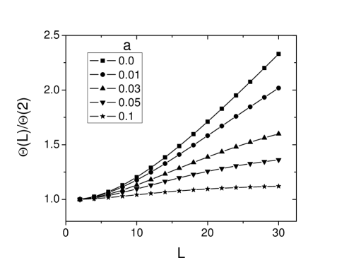
Figure 2: Moments of inertia $\Theta(L)$ for the ground state band, given by Eq. (120) and normalized to $\Theta(2)$, are shown for the specific values of $\beta_{0}=2$ and $c=5$, and varying parameter $a$. See Section XI for further discussion.

XI Numerical results

From Eq. (LABEL:eq:mBohr) it is clear that in the present case the moments of inertia are not proportional to $\beta^{2}\sin^{2}\left(\gamma-2\pi k/3\right)$ but to $(\beta^{2}/f^{2}(\beta))\sin^{2}\left(\gamma-2\pi k/3\right)$. The function $\beta^{2}/f^{2}(\beta)$ is shown in Fig. 1 for different values of the parameter $a$. It is clear that the increase of the moment of inertia is slowed down by the function $f(\beta)$, as it is expected as nuclear deformation sets in Ring .

The effect of the deformation-dependent mass on the moments of inertia can be seen in Fig. 2, where the moments of inertia Ring for the ground state band

$$\Theta(L)={2L-1\over E(L)-E(L-2)},$$ (120)

normalized to $\Theta(2)$, are shown in the case of axially symmetric prolate deformed nuclei, for the specific values of $\beta_{0}=2$ and $c=5$, and varying parameter $a$. It is clear that the rapid increase of the moments of inertia with $L$, seen for $a=0$, is gradually moderated by increasing $a$.

XI.1 Spectra of $\gamma$-unstable nuclei

Rms fits of spectra have been performed, using the quality measure

$$\sigma=\sqrt{{\sum_{i=1}^{n}(E_{i}(exp)-E_{i}(th))^{2}\over(n-1)E(2_{1}^{+})^{2}}}.$$ (121)

The theoretical predictions for the levels of the ground state band are obtained from Eq. (83), while the levels of the quasi-$\beta_{1}$ band are obtained from Eq. (84). The levels of the quasi-$\gamma_{1}$ band are obtained through their degeneracies to members of the ground state band, mentioned below Eq. (IV.1).

The results shown in Table 1 have been obtained for $\delta=\lambda=0$. (The Xe and Ba isotopes have already been considered in Ref. first .) One can easily verify that different choices for $\delta$ and $\lambda$ lead to a renormalization of the parameter values $a$ and $\beta_{0}$, the predicted energy levels remaining exactly the same.

Concerning the physical content of the parameter $a$, it is instructive to consider in detail in Table 1 the Xe isotopes (already discussed in Ref. first ), known Casten to lie in a $\gamma$-unstable region. They extend from the borders of the neutron shell (¹³⁴Xe₈₀ is just below the N=82 shell closure) to the midshell (¹²⁰Xe₆₆) and even beyond, exhibiting increasing collectivity (increasing $R_{4/2}=E(4_{1}^{+})/E(2_{1}^{+})$ ratios) from the border to the mishell. Moving from the border of the neutron shell to the midshell, the following remarks apply

i) ¹³⁴Xe and ¹³²Xe are almost pure vibrators. Therefore no need for deformation dependence of the mass exists, the least square fitting leading to $a=0$. Furthermore, no $\beta_{0}$ term is needed in the potential, the fitting therefore leading to $\beta_{0}=0$, i.e., to pure harmonic behaviour.

ii) In the next two isotopes (¹³⁰Xe and ¹²⁸Xe) the need to depart from the pure harmonic oscillator becomes clear, the fitting leading therefore to nonzero $\beta_{0}$ values. However, there is still no need of dependence of the mass on the deformation, the fitting still leading to $a=0$.

iii) Beyond ¹²⁶Xe both the $\beta_{0}$ term in the potential and the deformation dependence of the mass become necessary, leading to nonzero values of both $\beta_{0}$ and $a$.

Other chains of isotopes also show similar behavior.

XI.2 Spectra of axially symmetric deformed nuclei

Fits of spectra of deformed rare earth and actinide nuclei are shown in Table 2. The energy levels of the ground state band and the $\beta_{1}$ band (both having $n_{\gamma}=0$ and $K=0$) are obtained from Eqs. (83) and (84) respectively, while the levels of the $\gamma_{1}$ band are obtained from Eq. (83) with $n_{\gamma}=1$ and $K=2$. Again, the choice $\delta=\lambda=0$ has been made, and it is seen that different choices for $\delta$ and $\lambda$ lead to a renormalization of the parameter values $a$, $\beta_{0}$, and $c$, the predicted energy levels remaining exactly the same.

The quality of the fits obtained can also be seen in Table 3, where the calculated energy levels of ¹⁶²Dy and ²³⁸U are compared to experiment.

The following remarks apply.

1) Both the bandheads and the spacings within bands are in general well reproduced. This is particularly true for the ground state and the $\gamma_{1}$ bands. The deviation in the gsb of ¹⁶²Dy reaches 0.6% at $L=18$, while in the gsb of ²³⁸U it reaches 1.7% at $L=30$. The experimental levels of the $\gamma_{1}$ band of ¹⁶²Dy (up to $L=14$) extend over 28.4 energy units, while the corresponding theoretical predictions spread over 28.7 units, the difference being of the order of 1%. Similarly in ²³⁸U the experimental spread of the $\gamma_{1}$ band (up to $L=27$) is 89.1 energy units, while the theoretical one is 87.3 units, the difference being of the order of 2%.

2) However we remark that the theoretical level spacings within the $\beta_{1}$ bands are larger than the experimental ones. This should be attributed to the shape of the Davidson potential, which raises to infinity at large $\beta$, pushing $\beta$ bands higher and increasing their interlevel spacing. It is known that this problem can be avoided by using a potential going to some finite value at large $\beta$ finitew , like the Morse potential Morse .

XI.3 $B(E2)$s of $\gamma$-unstable nuclei

$B(E2)$s within the ground state band, as well as interband $B(E2)$s for which experimental data exist for several nuclei, have been calculated using the procedure described in subsec. X.A . The results are shown in Table 4, the overall agreement being good.

XI.4 $B(E2)$s of axially symmetric deformed nuclei

$B(E2)$s within the ground state band, as well as interband $B(E2)$s for which experimental data exist for several nuclei, have been calculated using the procedure described in subsec. X.B . The results are shown in Table 5. The overall agreement is good for transitions within the ground state band (gsb), as well as for transitions connecting the $\gamma_{1}$ band to the gsb, while transitions from the $\beta_{1}$ band to the gsb tend to be overpredicted. One should remember at this point that the $\beta_{1}$ band was the one giving poor results also in the case of the spectra, in subsec. XI.B .

XII Connection to earlier work

It is instructive to examine the relation between the present approach and earlier numerical work.

1) The formalism of subsection III.B clarifies the relation between the present approach and the numerical solution of Kumar and Baranger Kumar , who used a matrix of the form (14) with $g_{ij}$, $i,j=1,2,3$ the same as in Eq. (15), but with

$$g_{44}=B_{00},\quad g_{55}=B_{2^{\prime}2^{\prime}},\quad g_{45}=g_{54}=B_{02^{\prime}},$$ (122)

where $B_{00}$, $B_{2^{\prime}2^{\prime}}$, $B_{02^{\prime}}$, as well as the moments of inertia ${\cal J}_{i}$ ($i=1,2,3$) and the potential $V$ have been treated as seven arbitrary functions of the variables $\beta_{0}=\beta\cos\gamma$ and $\beta_{2^{\prime}}=\beta\sin\gamma$ [while in the Bohr formulation Bohr $a_{0}=\beta\cos\gamma$ and $a_{2}=\beta\sin\gamma/\sqrt{2}$ are used]. On one hand, the present solution is a special case of Ref. Kumar , since it contains no non-diagonal terms $g_{45}=g_{54}$. On the other hand, in the present approach the above mentioned quantities are interrelated by the overall symmetry in a specific way, greatly reducing the number of free parameters (down to two or three in total). It should be pointed out that the functional dependence of the mass on the deformation for the potential used is dictated by SUSYQM. Therefore, the successful prediction of the behavior of the moments of inertia, for example, provides credit for the present approach. What we see, independently of the parameter values, is that the increase of the moments of inertia as a function of deformation is moderated by the $f^{2}$ factor, which can be seen as a result of the dependence of the mass on the deformation, or, alternatively, as seen in subsection III.B, as a result of using a curved space.

2) It should be pointed out that in Ref. QT4267 the equivalence between the position dependent mass case and the curved space approach has been established in the special case of $\kappa=2$ and $\delta=\lambda=0$ (see Eq. (II) for the meaning of the symbols), which represents the BenDaniel and Duke Hamiltonian BenD

$$H_{BD}=-{\hbar^{2}\over 2}\nabla f^{2}\nabla+V_{BD}.$$ (123)

This resembles the collective Hamiltonian

$$H_{coll}=-{\hbar^{2}\over 2}\Sigma_{i,j}{\partial\over\partial q_{i}}[{\cal M}(q)_{ij}]^{-1}{\partial\over\partial q_{j}}+V(q)$$ (124)

used by Libert et al. Libert in mean field calculations, in which a tensor mass appears.

XIII Conclusion

In the present work analytical solutions are obtained for a Bohr Hamiltonian in which the mass has been allowed to depend on the deformation.

From the mathematical point of view, this is achieved through the use of techniques of supersymmetric quantum mechanics PR ; SUSYQM , involving a deformed shape invariance condition Q2929 . Analytical expressions for the spectra and wave functions have been obtained.

From the physics point of view, spectra and $B(E2)$ transition rates have been calculated for $\gamma$-unstable, axially symmetric prolate deformed, and triaxial nuclei, implementing the usual approximations in each case, and compared to experimental data for the first two cases. The main new result is that the dependence of the mass on the deformation moderates the increase of the moment of inertia with the deformation, removing an important drawback Ring of the model. It should be emphasized that the functional dependence of the mass on the deformation for the potential used is dictated by SUSYQM, thus the correction in the behavior of the moments of inertia is a general effect, independent of any specific parameter value combinations.

However, certain discrepancies with experimental data remain, especially related to the $\beta_{1}$-band and its interband transitions. It should be remembered at this point that in the present study separation of variables has been achieved by assuming that the potential either is independent of the $\gamma$-variable, or it has the exactly separable form of Eq. (34). Furthermore, the approximations related to Eqs. (IV.2) and (44) have been implemented. Recently, the numerical solution of the Bohr Hamiltonian for any value of $\beta$ and $\gamma$, avoiding all these approximations, has been achieved in the framework of the powerful algebraic collective model Rowe ; Turner ; Welsh . The detailed study of discrepancies from experimental data both in the SUSYQM framework and in the context of the algebraic model, especially for multi-phonon excitations Caprio2 , could shed light on the origins of these discrepancies.

As it has already been mentioned, the form of the dependence of the mass on the deformation is dictated by SUSYQM for the potential used in the $\beta$ degree of freedom. In the present work, the Davidson potential has been used, called the Deformation Dependent Mass (DDM) Davidson model. The application of the SUSYQM approach to the Bohr Hamiltonian with the Kratzer potential FV1 ; FV2 is receiving attention.

Appendix 1

When using Eq. (112) in numerical calculations, problems can appear because of $\Gamma(x)$ functions with large $x$. These problems can be avoided by using Eq. 6.1.16 of Ref. AbrSte

$$\Gamma(n+z)=(n-1+z)(n-2+z)\dots(1+z)\Gamma(1+z).$$ (125)

In the normalization factors we need the ratio of

$$\Gamma\left(n+{\Delta_{1}+\Delta_{2}\over 2}+1\right)$$ (126)

over

$$\Gamma\left(n+{\Delta_{2}\over 2}+1\right).$$ (127)

Let us call $I$ the integer part of $\Delta_{2}/2$ and $r$ the rest of it, i.e.,

$${\Delta_{2}\over 2}=I+r.$$ (128)

Then we have

$$\begin{split}&\Gamma\left(n+{\Delta_{1}+\Delta_{2}\over 2}+1\right)=\Gamma\left(I+(n+\Delta_{1}/2+r+1)\right)\\ &=(I-1+n+\Delta_{1}/2+r+1)\\ &(I-2+n+\Delta_{1}/2+r+1)\dots(1+n+\Delta_{1}/2+r+1)\\ &\Gamma(1+n+\Delta_{1}/2+r+1),\end{split}$$ (129)

$$\begin{split}&\Gamma\left(n+{\Delta_{2}\over 2}+1\right)=\Gamma\left(I+(n+r+1)\right)\\ &=(I-1+n+r+1)(I-2+n+r+1)\dots\\ &(1+n+r+1)\Gamma(1+n+r+1).\end{split}$$ (130)

Their ratio becomes

$$\begin{split}&{\Gamma\left(n+{\Delta_{1}+\Delta_{2}\over 2}+1\right)\over\Gamma\left(n+{\Delta_{2}\over 2}+1\right)}={(I-1+n+\Delta_{1}/2+r+1)\over(I-1+n+r+1)}\\ &{(I-2+n+\Delta_{1}/2+r+1)\over(I-2+n+r+1)}\dots(1+n+\Delta_{1}/2+r+1)\over(1+n+r+1)\\ &{\Gamma(1+n+\Delta_{1}/2+r+1)\over\Gamma(1+n+r+1)}\\ &=\left(1+{\Delta_{1}/2\over(I-1+n+r+1)}\right)\\ &\left(1+{\Delta_{1}/2\over(I-2+n+r+1)}\right)\dots\left(1+{\Delta_{1}/2\over(1+n+r+1)}\right)\\ &{\Gamma(1+n+\Delta_{1}/2+r+1)\over\Gamma(1+n+r+1)},\end{split}$$ (131)

in which one does not have to calculate $\Gamma(x)$ functions with large $x$. The only large numbers appear in denominators of fractions accompanying 1, which do not pose any problem.

Table 1: Comparison of theoretical predictions of the $\gamma$-unstable Bohr Hamiltonian with $\beta$-dependent mass (with $\delta=\lambda=0$) to experimental data NDS of rare earth and actinide nuclei with $R_{4/2}\leq 2.6$ and known $0_{2}^{+}$ and $2_{\gamma}^{+}$ states. The $R_{4/2}=E(4_{1}^{+})/E(2_{1}^{+})$ ratios, as well as the $\beta$ and $\gamma$ bandheads, normalized to the $2_{1}^{+}$ state and labelled by $R_{0/2}=E(0_{\beta}^{+})/E(2_{1}^{+})$ and $R_{2/2}=E(2_{\gamma}^{+})/E(2_{1}^{+})$ respectively, are shown. $\beta_{0}$ and $a$ are free parameters, related to the Davidson potential [Eq. (58)] and to the dependence of the mass on the deformation [Eq. (59)]. The angular momenta of the highest levels of the ground state, $\beta$ and $\gamma$ bands included in the rms fit are labelled by $L_{g}$, $L_{\beta}$, and $L_{\gamma}$ respectively, while $n$ indicates the total number of levels involved in the fit and $\sigma$ is the quality measure of Eq. (121). The theoretical predictions are obtained from the formulae mentioned below Eq. (121). The Xe and Ba isotopes have already been considered in Ref. first . See subsec. XI.1 for further discussion.

nucleus	$R_{4/2}$	$R_{4/2}$	$R_{0/2}$	$R_{0/2}$	$R_{2/2}$	$R_{2/2}$	$\beta_{0}$	$a$	$L_{g}$	$L_{\beta}$	$L_{\gamma}$	$n$	$\sigma$
	exp	th	exp	th	exp	th
98Ru	2.14	2.14	2.0	2.4	2.2	2.1	0.99	0.020	24	0	4	15	0.277
100Ru	2.27	2.24	2.1	2.7	2.5	2.2	1.19	0.048	28	0	4	17	0.315
102Ru	2.33	2.20	2.0	2.4	2.3	2.2	1.05	0.059	16	0	5	12	0.364
104Ru	2.48	2.34	2.8	3.0	2.5	2.3	1.40	0.083	8	2	8	12	0.429
102Pd	2.29	2.24	2.9	2.3	2.8	2.2	1.08	0.081	26	4	4	18	0.326
104Pd	2.38	2.21	2.4	2.6	2.4	2.2	1.15	0.034	18	2	4	13	0.397
106Pd	2.40	2.16	2.2	2.2	2.2	2.2	0.91	0.062	16	4	5	14	0.409
108Pd	2.42	2.26	2.4	2.3	2.1	2.3	1.09	0.103	14	4	4	12	0.318
110Pd	2.46	2.31	2.5	2.0	2.2	2.3	0.99	0.195	12	10	4	14	0.354
112Pd	2.53	2.29	2.6	2.5	2.1	2.3	1.21	0.086	6	0	3	5	0.485
114Pd	2.56	2.31	2.6	2.8	2.1	2.3	1.30	0.076	16	0	11	18	0.722
116Pd	2.58	2.36	3.3	3.4	2.2	2.4	1.52	0.062	16	0	9	16	0.609
106Cd	2.36	2.25	2.8	2.9	2.7	2.3	1.28	0.028	12	0	2	7	0.268
108Cd	2.38	2.14	2.7	2.2	2.5	2.1	0.91	0.041	24	0	5	16	0.528
110Cd	2.35	2.08	2.2	1.9	2.2	2.1	0.00	0.061	16	6	5	15	0.415
112Cd	2.29	2.05	2.0	1.9	2.1	2.0	0.00	0.033	12	8	11	20	0.523
114Cd	2.30	2.06	2.0	1.9	2.2	2.1	0.00	0.041	14	4	3	11	0.418
116Cd	2.38	2.16	2.5	2.7	2.4	2.2	1.14	0.000	14	2	3	10	0.387
118Cd	2.39	2.19	2.6	2.9	2.6	2.2	1.21	0.002	14	0	3	9	0.429
120Cd	2.38	2.20	2.7	2.9	2.6	2.2	1.22	0.006	16	0	2	9	0.412
118Xe	2.40	2.32	2.5	2.6	2.8	2.3	1.27	0.103	16	4	10	19	0.319
120Xe	2.47	2.36	2.8	3.4	2.7	2.4	1.51	0.063	26	4	9	23	0.524
122Xe	2.50	2.40	3.5	3.3	2.5	2.4	1.57	0.096	16	0	9	16	0.638
124Xe	2.48	2.36	3.6	3.5	2.4	2.4	1.55	0.051	20	2	11	21	0.554
126Xe	2.42	2.33	3.4	3.1	2.3	2.3	1.42	0.064	12	4	9	16	0.584
128Xe	2.33	2.27	3.6	3.5	2.2	2.3	1.42	0.000	10	2	7	12	0.431
130Xe	2.25	2.21	3.3	3.1	2.1	2.2	1.27	0.000	14	0	5	11	0.347
132Xe	2.16	2.00	2.8	2.0	1.9	2.0	0.00	0.000	6	0	5	7	0.467
134Xe	2.04	2.00	1.9	2.0	1.9	2.0	0.00	0.000	6	0	5	7	0.685
130Ba	2.52	2.42	3.3	3.2	2.5	2.4	1.60	0.118	12	0	6	11	0.352
132Ba	2.43	2.29	3.2	2.8	2.2	2.3	1.29	0.059	14	0	8	14	0.619
134Ba	2.32	2.16	2.9	2.7	1.9	2.2	1.12	0.000	8	0	4	7	0.332
136Ba	2.28	2.00	1.9	2.0	1.9	2.0	0.00	0.000	6	0	2	4	0.250
142Ba	2.32	2.38	4.3	4.3	4.0	2.4	1.72	0.028	14	0	2	8	0.609
134Ce	2.56	2.34	3.7	3.9	2.4	2.3	1.59	0.019	34	2	8	25	0.527
136Ce	2.38	2.11	1.9	2.1	2.0	2.1	0.82	0.034	16	0	3	10	0.457
138Ce	2.32	2.00	1.9	2.0	1.9	2.0	0.00	0.000	14	0	2	8	0.314
140Nd	2.33	2.05	1.8	1.9	1.9	2.1	0.00	0.037	6	0	2	4	0.192
148Nd	2.49	2.36	3.0	2.8	4.1	2.4	1.38	0.110	12	8	4	13	0.764
140Sm	2.35	2.29	1.9	1.9	2.7	2.3	0.92	0.196	8	0	2	5	0.207
142Sm	2.33	2.06	1.9	1.9	2.2	2.1	0.33	0.044	8	0	2	5	0.147
142Gd	2.35	2.21	2.7	2.8	1.9	2.2	1.20	0.020	16	0	2	9	0.231
144Gd	2.35	2.33	2.5	2.5	2.5	2.3	1.26	0.112	6	0	2	4	0.124
152Gd	2.19	2.13	1.8	1.8	3.2	2.1	0.00	0.104	16	10	7	19	0.635
154Dy	2.23	2.15	2.0	2.0	3.1	2.1	0.75	0.083	26	10	7	24	0.530
156Er	2.32	2.25	2.7	2.8	2.7	2.3	1.24	0.043	20	4	5	16	0.450

Table 1: (continued)

nucleus	$R_{4/2}$	$R_{4/2}$	$R_{0/2}$	$R_{0/2}$	$R_{2/2}$	$R_{2/2}$	$\beta_{0}$	$a$	$L_{g}$	$L_{\beta}$	$L_{\gamma}$	$n$	$\sigma$
	exp	th	exp	th	exp	th
186Pt	2.56	2.42	2.5	3.7	3.2	2.4	1.71	0.085	26	6	10	25	0.813
188Pt	2.53	2.37	3.0	3.3	2.3	2.4	1.52	0.076	16	2	4	12	0.637
190Pt	2.49	2.28	3.1	3.4	2.0	2.3	1.42	0.015	18	2	6	15	0.637
192Pt	2.48	2.34	3.8	3.7	1.9	2.3	1.56	0.032	10	0	8	12	0.681
194Pt	2.47	2.36	3.9	3.6	1.9	2.4	1.55	0.049	10	4	5	11	0.667
196Pt	2.47	2.33	3.2	2.9	1.9	2.3	1.37	0.079	10	2	6	11	0.639
198Pt	2.42	2.21	2.2	2.2	1.9	2.2	0.96	0.089	6	2	4	7	0.370
200Pt	2.35	2.00	2.4	2.0	1.8	2.0	0.00	0.000	4	0	4	5	0.392

Table 2: Same as Table 1, but for axially symmetric prolate deformed rare earth and actinide nuclei with $R_{4/2}$ $>$ 2.9 . $\beta_{0}$, $a$, and $c$ are free parameters, related to the Davidson potential [Eq. (58)], to the dependence of the mass on the deformation [Eq. (59)], and to the $\gamma$-potential [Eq. (40)]. The theoretical predictions are obtained from the equations mentioned in subsec. XI.2, where further discussion can be found.

nucleus	$R_{4/2}$	$R_{4/2}$	$R_{0/2}$	$R_{0/2}$	$R_{2/2}$	$R_{2/2}$	$\beta_{0}$	$c$	$a$	$L_{g}$	$L_{\beta}$	$L_{\gamma}$	$n$	$\sigma$
	exp	th	exp	th	exp	th
150Nd	2.93	3.13	5.2	7.9	8.2	5.8	0.0	2.1	0.003	14	6	4	13	2.012
152Sm	3.01	3.14	5.6	8.4	8.9	6.5	0.0	2.4	0.000	16	14	9	23	3.327
154Sm	3.25	3.27	13.4	13.0	17.6	18.6	1.30	6.9	0.021	16	6	7	17	0.515
154Gd	3.02	3.09	5.5	6.5	8.1	4.1	0.0	1.4	0.024	26	26	7	32	3.546
156Gd	3.24	3.25	11.8	10.8	13.0	14.3	0.0	5.3	0.026	26	12	16	34	0.933
158Gd	3.29	3.29	15.0	14.5	14.9	15.1	1.99	5.3	0.025	12	6	6	14	0.323
160Gd	3.30	3.30	17.6	17.3	13.1	13.2	2.38	4.5	0.020	16	4	8	17	0.125
162Gd	3.29	3.30	19.8	19.8	12.0	12.1	2.52	4.1	0.008	14	0	4	10	0.078
156Dy	2.93	3.13	4.9	7.4	6.5	5.3	0.0	1.9	0.014	28	10	13	31	1.789
158Dy	3.21	3.22	10.0	9.6	9.6	10.3	0.26	3.8	0.023	28	8	8	25	0.496
160Dy	3.27	3.27	14.7	14.7	11.1	12.1	1.92	4.3	0.005	28	4	23	38	0.510
162Dy	3.29	3.30	17.3	15.7	11.0	11.2	2.23	3.8	0.020	18	8	14	26	0.742
164Dy	3.30	3.30	22.6	22.5	10.4	10.2	2.68	3.4	0.000	20	0	10	19	0.100
166Dy	3.31	3.31	15.0	14.9	11.2	11.2	2.39	3.7	0.047	6	2	5	8	0.077
160Er	3.10	3.16	7.1	8.1	6.8	6.6	0.00	2.4	0.013	26	2	5	18	0.699
162Er	3.23	3.23	10.7	10.7	8.8	10.1	1.29	3.7	0.013	20	4	12	23	0.770
164Er	3.28	3.27	13.6	12.2	9.4	9.6	1.83	3.3	0.026	22	10	18	33	0.918
166Er	3.29	3.28	18.1	16.8	9.8	9.9	2.22	3.4	0.002	16	10	14	26	0.698
168Er	3.31	3.31	15.3	14.4	10.3	10.2	2.29	3.4	0.041	18	6	8	19	0.404
170Er	3.31	3.30	11.3	10.1	11.9	12.9	1.64	4.4	0.083	24	10	19	35	0.837
162Yb	2.92	3.07	3.6	6.8	4.8	4.0	0.00	1.4	0.003	24	0	4	15	1.036
164Yb	3.13	3.18	7.9	8.3	7.0	7.4	0.00	2.7	0.023	18	0	5	13	0.357
166Yb	3.23	3.23	10.2	8.9	9.1	9.7	0.66	3.5	0.038	24	10	13	29	0.973
168Yb	3.27	3.26	13.2	11.2	11.2	11.5	1.52	4.1	0.028	34	4	7	25	1.070
170Yb	3.29	3.27	12.7	11.2	13.6	14.1	1.36	5.1	0.035	20	10	17	31	0.963
172Yb	3.31	3.30	13.2	12.2	18.6	18.9	1.66	6.6	0.055	16	10	5	17	0.742
174Yb	3.31	3.31	19.4	19.3	21.4	21.5	2.44	7.5	0.019	20	4	5	16	0.104
176Yb	3.31	3.30	13.9	13.7	15.4	15.5	1.97	5.4	0.036	20	2	5	15	0.287
178Yb	3.31	3.27	15.7	15.5	14.5	14.6	1.88	5.3	0.000	6	4	2	6	0.127
166Hf	2.97	3.08	4.4	6.9	5.1	4.3	0.00	1.5	0.006	22	0	3	13	0.873
168Hf	3.11	3.17	7.6	8.1	7.1	6.9	0.00	2.5	0.023	22	4	4	16	0.494
170Hf	3.19	3.21	8.7	8.7	9.5	8.8	0.00	3.2	0.033	34	4	4	22	0.970
172Hf	3.25	3.24	9.2	9.8	11.3	11.7	0.00	4.3	0.031	38	4	6	26	0.549
174Hf	3.27	3.25	9.1	10.4	13.5	13.6	0.00	5.0	0.033	26	4	5	19	0.832
176Hf	3.28	3.28	13.0	11.5	15.2	16.1	1.31	5.8	0.038	18	10	8	21	0.950
178Hf	3.29	3.28	12.9	12.3	12.6	13.0	1.70	4.6	0.028	18	6	6	17	0.356
180Hf	3.31	3.30	11.8	11.5	12.9	13.0	1.92	4.4	0.068	12	4	5	12	0.157
176W	3.22	3.21	7.8	9.1	9.6	9.5	0.00	3.5	0.027	22	4	5	17	0.881
178W	3.24	3.22	9.4	8.6	10.5	8.9	0.00	3.2	0.039	18	10	2	15	0.987
180W	3.26	3.25	14.6	13.1	10.8	11.5	1.64	4.2	0.000	24	0	7	18	0.603
182W	3.29	3.29	11.3	11.5	12.2	12.5	1.77	4.3	0.050	18	4	6	16	0.195
184W	3.27	3.28	9.0	8.9	8.1	8.0	1.57	2.7	0.080	10	4	6	12	0.093
186W	3.23	3.25	7.2	7.2	6.0	6.3	1.20	2.1	0.099	14	4	6	14	0.130
176Os	2.93	3.10	4.5	6.9	6.4	4.6	0.00	1.6	0.016	24	6	5	19	1.747
178Os	3.02	3.12	4.9	7.2	6.6	5.1	0.00	1.8	0.017	16	6	5	15	1.836
180Os	3.09	3.22	5.6	7.1	6.6	6.9	0.00	2.4	0.078	10	6	7	14	1.021
184Os	3.20	3.21	8.7	9.9	7.9	8.5	1.21	3.1	0.011	22	0	6	16	0.886
186Os	3.17	3.19	7.7	7.0	5.6	6.0	0.00	2.1	0.063	14	10	13	24	0.702
188Os	3.08	3.15	7.0	7.2	4.1	4.4	1.07	1.5	0.033	12	2	7	13	0.170
190Os	2.93	3.07	4.9	5.6	3.0	3.1	0.00	1.0	0.051	10	2	6	11	0.419

Table 2: (continued)

nucleus	$R_{4/2}$	$R_{4/2}$	$R_{0/2}$	$R_{0/2}$	$R_{2/2}$	$R_{2/2}$	$\beta_{0}$	$c$	$a$	$L_{g}$	$L_{\beta}$	$L_{\gamma}$	$n$	$\sigma$
	exp	th	exp	th	exp	th
228Ra	3.21	3.24	11.3	11.0	13.3	13.3	0.57	5.0	0.016	22	4	3	15	0.177
228Th	3.24	3.26	14.4	14.3	16.8	17.0	1.50	6.4	0.002	18	2	5	14	0.214
230Th	3.27	3.27	11.9	11.6	14.7	14.7	1.44	5.3	0.034	24	4	4	17	0.243
232Th	3.28	3.28	14.8	14.0	15.9	16.5	1.80	5.9	0.022	30	10	12	31	0.426
232U	3.29	3.29	14.5	13.8	18.2	18.4	1.74	6.6	0.028	20	10	4	18	0.394
234U	3.30	3.30	18.6	18.3	21.3	21.8	2.19	7.8	0.011	28	8	7	24	0.244
236U	3.30	3.30	20.3	20.0	21.2	21.2	2.38	7.5	0.009	30	4	5	21	0.143
238U	3.30	3.31	20.6	20.6	23.6	24.7	2.38	8.8	0.009	30	4	27	43	0.665
238Pu	3.31	3.31	21.4	21.4	23.3	23.3	2.61	8.1	0.016	26	2	4	17	0.067
240Pu	3.31	3.31	20.1	19.9	26.6	26.6	2.40	9.4	0.018	26	4	4	18	0.117
242Pu	3.31	3.31	21.5	21.4	24.7	24.7	2.52	8.7	0.012	26	2	2	15	0.107
248Cm	3.31	3.31	25.0	24.8	24.2	24.3	2.72	8.5	0.004	28	4	2	17	0.159
250Cf	3.32	3.31	27.0	26.9	24.2	24.2	2.88	8.4	0.003	8	2	4	8	0.053

Table 3: Normalized [to the energy of the first excited state, $E(2_{1}^{+})$] energy levels of the ground state band (gsb) and the $\beta_{1}$ and $\gamma_{1}$ bands of ¹⁶²Dy and ²³⁸U, obtained from the Bohr Hamiltonian with $\beta$-dependent mass for axially symmetric prolate deformed nuclei using the parameters given in Table 2, compared to experimental data NDS . See subsec. XI.2 for further discussion.

	162Dy	162Dy	238U	238U		162Dy	162Dy	238U	238U
L	exp	th	exp	th	L	exp	th	exp	th
	gsb	gsb	gsb	gsb		$\gamma_{1}$	$\gamma_{1}$	$\gamma_{1}$	$\gamma_{1}$
0	0.00	0.00	0.00	0.00	2	11.0	11.2	23.6	24.7
2	1.00	1.00	1.00	1.00	3	11.9	12.1	24.6	25.5
4	3.29	3.30	3.30	3.31	4	13.2	13.3	25.9	26.7
6	6.80	6.80	6.84	6.86	5	14.7	14.7	27.4	28.1
8	11.41	11.41	11.54	11.57	6	16.4	16.5	29.2	29.8
10	17.04	17.01	17.27	17.33	7	18.5	18.5	31.2	31.7
12	23.57	23.49	23.97	24.06	8	20.7	20.8	33.5	33.9
14	30.90	30.74	31.51	31.63	9	23.3	23.3	36.0	36.3
16	38.90	38.70	39.82	39.97	10	25.9	26.0	38.8	39.0
18	47.58	47.28	48.78	48.98	11	29.0	28.9	41.7	41.9
20			58.31	58.61	12	31.4	32.1	44.9	45.0
22			68.31	68.77	13	35.5	35.5	48.3	48.3
24			78.71	79.44	14	39.4	39.9	51.9	51.8
26			89.46	90.55	15			55.7	55.5
28			100.57	102.08	16			59.7	59.4
30			112.10	113.99	17			63.9	63.4
					18			68.2	67.7
	$\beta_{1}$	$\beta_{1}$	$\beta_{1}$	$\beta_{1}$	19			72.7	72.0
0	17.3	15.7	20.6	20.6	20			77.3	76.6
2	18.0	16.7	21.5	21.6	21			82.1	81.3
4	19.5	19.0	23.5	24.0	22			87.0	86.1
6	21.9	22.6			23			91.9	91.0
8	24.6	27.4			24			97.0	96.1
					25			102.1	101.3
					26			107.4	106.6
					27			112.7	112.0

Table 4: Comparison of experimental data NDS (upper line) for several $B(E2)$ ratios of $\gamma$-unstable nuclei to predictions (lower line) by the Bohr Hamiltonian with $\beta$-dependent mass (with $\delta=\lambda=0$), for the parameter values shown in Table 1. See subsec. XI.3 for further discussion.

nucl.	$4_{1}\to 2_{1}\over 2_{1}\to 0_{1}$		$6_{1}\to 4_{1}\over 2_{1}\to 0_{1}$		$8_{1}\to 6_{1}\over 2_{1}\to 0_{1}$		$10_{1}\to 8_{1}\over 2_{1}\to 0_{1}$		$2_{2}\to 2_{1}\over 2_{1}\to 0_{1}$		$2_{2}\to 0_{1}\over 2_{1}\to 0_{1}$		$0_{2}\to 2_{1}\over 2_{1}\to 0_{1}$		$2_{3}\to 0_{1}\over 2_{1}\to 0_{1}$
											x $10^{3}$				x $10^{3}$
98Ru	1.	44(25)							1.	62(61)	36.	0(152)
	1.	82	2.	62	3.	42	4.	22	1.	82	0.	0	1.	36	3.	60
100Ru	1.	45(13)							0.	64(12)	41.	1(52)	0.	98(15)
	1.	72	2.	40	3.	07	3.	73	1.	72	0.	0	1.	05	10.	89
102Ru	1.	50(24)							0.	62(7)	24.	8(7)	0.	80(14)
	1.	78	2.	54	3.	28	4.	01	1.	78	0.	0	1.	27	8.	70
104Ru	1.	18(28)							0.	63(15)	35.	0(84)	0.	42(7)
	1.	63	2.	18	2.	71	3.	21	1.	63	0.	0	0.	79	22.	41
102Pd	1.	56(19)							0.	46(9)	128.	8(735)
	1.	76	2.	49	3.	19	3.	87	1.	76	0.	0	1.	22	12.	34
104Pd	1.	36(27)							0.	61(8)	33.	3(74)
	1.	74	2.	45	3.	15	3.	85	1.	74	0.	0	1.	11	8.	13
106Pd	1.	63(28)							0.	98(12)	26.	2(31)	0.	67(18)
	1.	85	2.	67	3.	49	4.	28	1.	85	0.	0	1.	49	5.	98
108Pd	1.	47(20)	2.	16(28)	2.	99(48)			1.	43(14)	16.	6(18)	1.	05(13)	1.	90(29)
	1.	75	2.	45	3.	12	3.	75	1.	75	0.	0	1.	20	15.	82
110Pd	1.	71(34)							0.	98(24)	14.	1(22)	0.	64(10)
	1.	76	2.	43	3.	01	3.	51	1.	76	0.	0	1.	31	26.	24
106Cd	1.	78(25)							0.	43(12)	93.	0(127)
	1.	68	2.	32	2.	95	3.	58	1.	68	0.	0	0.	92	10.	44
108Cd	1.	54(24)							0.	64(20)	67.	7(120)
	1.	85	2.	69	3.	52	4.	35	1.	85	0.	0	1.	49	4.	06
110Cd	1.	68(24)							1.	09(19)	48.	9(78)			9.	85(595)
	1.	99	2.	97	3.	93	4.	87	1.	99	0.	0	1.	98	1.	61
112Cd	2.	02(22)							0.	50(10)	19.	9(35)	1.	69(48)	11.	26(210)
	2.	00	2.	99	3.	98	4.	96	2.	00	0.	0	1.	99	0.	48
114Cd	1.	99(25)	3.	83(72)	2.	73(97)			0.	71(24)	15.	4(29)	0.	88(11)	10.	61(193)
	2.	00	2.	99	3.	97	4.	94	2.	00	0.	0	1.	99	0.	74
116Cd	1.	70(52)							0.	63(46)	32.	8(86)	0.	02
	1.	74	2.	46	3.	17	3.	90	1.	74	0.	0	1.	11	4.	42
118Cd	$>$1.	85											0.	16(4)
	1.	71	2.	39	3.	06	3.	74	1.	71	0.	0	1.	00	5.	88
118Xe	1.	11(7)	0.	88(27)	0.	49(20)	$>$0.	73
	1.	67	2.	28	2.	85	3.	39	1.	67	0.	0	0.	95	21.	93
120Xe	1.	16(14)	1.	17(24)	0.	96(22)	0.	91(19)
	1.	60	2.	11	2.	60	3.	08	1.	60	0.	0	0.	67	21.	51
122Xe	1.	47(38)	0.	89(26)	$>$0.	44
	1.	58	2.	05	2.	48	2.	89	1.	58	0.	0	0.	63	29.	29
124Xe	1.	34(24)	1.	59(71)	0.	63(29)	0.	29(8)	0.	70(19)	15.	9(46)
	1.	59	2.	09	2.	57	3.	04	1.	59	0.	0	0.	63	20.	14
128Xe	1.	47(20)	1.	94(26)	2.	39(40)	2.	74(114)	1.	19(19)	15.	9(23)
	1.	63	2.	20	2.	75	3.	31	1.	63	0.	0	0.	73	9.	64
132Xe	1.	24(18)							1.	77(29)	3.	4(7)
	2.	00	3.	00	4.	00	5.	00	2.	00	0.	0	2.	00	0.	00
130Ba	1.	36(6)	1.	62(15)	1.	55(56)	0.	93(15)
	1.	56	2.	01	2.	41	2.	77	1.	56	0.	0	0.	61	34.	54
132Ba									3.	35(64)	90.	7(177)
	1.	68	2.	30	2.	90	3.	50	1.	68	0.	0	0.	92	15.	21
134Ba	1.	55(21)							2.	17(69)	12.	5(41)
	1.	75	2.	48	3.	21	3.	94	1.	75	0.	0	1.	14	4.	08
142Ba	1.	40(17)	0.	56(14)
	1.	55	2.	00	2.	41	2.	82	1.	55	0.	0	0.	49	18.	60

Table 4: (continued)

nucl.	$4_{1}\to 2_{1}\over 2_{1}\to 0_{1}$		$6_{1}\to 4_{1}\over 2_{1}\to 0_{1}$		$8_{1}\to 6_{1}\over 2_{1}\to 0_{1}$		$10_{1}\to 8_{1}\over 2_{1}\to 0_{1}$		$2_{2}\to 2_{1}\over 2_{1}\to 0_{1}$		$2_{2}\to 0_{1}\over 2_{1}\to 0_{1}$		$0_{2}\to 2_{1}\over 2_{1}\to 0_{1}$		$2_{3}\to 0_{1}\over 2_{1}\to 0_{1}$
											x $10^{3}$				x $10^{3}$
148Nd	1.	61(13)	1.	76(19)					0.	25(4)	9.	3(17)	0.	54(6)	32.	82(816)
	1.	63	2.	17	2.	68	3.	15	1.	63	0.	0	0.	81	26.	86
152Gd	1.	84(29)	2.	74(81)					0.	23(4)	4.	2(8)	2.	47(78)
	1.	98	2.	92	3.	81	4.	65	1.	98	0.	0	1.	95	4.	51
154Dy	1.	62(35)	2.	05(42)	2.	27(62)	1.	86(69)
	1.	91	2.	79	3.	64	4.	46	1.	91	0.	0	1.	70	5.	41
156Er	1.	78(16)	1.	89(36)	0.	76(20)	0.	88(22)
	1.	70	2.	35	3.	00	3.	64	1.	70	0.	0	0.	98	11.	50
192Pt	1.	56(12)	1.	23(55)					1.	91(16)	9.	5(9)
	1.	59	2.	09	2.	57	3.	05	1.	59	0.	0	0.	61	16.	98
194Pt	1.	73(13)	1.	36(45)	1.	02(30)	0.	69(19)	1.	81(25)	5.	9(9)	0.	01
	1.	59	2.	09	2.	57	3.	04	1.	59	0.	0	0.	63	19.	78
196Pt	1.	48(3)	1.	80(23)	1.	92(23)					0.	4	0.	07(4)	0.	06(6)
	1.	64	2.	21	2.	75	3.	28	1.	64	0.	0	0.	82	20.	83
198Pt	1.	19(13)	$>$1.	78					1.	16(23)	1.	2(4)	0.	81(22)	1.	56(126)
	1.	82	2.	60	3.	36	4.	08	1.	82	0.	0	1.	41	10.	09

Table 5: Comparison of experimental data NDS (upper line) for several $B(E2)$ ratios of axially symmetric prolate deformed nuclei to predictions (lower line) by the Bohr Hamiltonian with $\beta$-dependent mass (with $\delta=\lambda=0$), for the parameter values shown in Table 2. See subsec. XI.4 for further discussion.

nucl.	$4_{1}\to 2_{1}\over 2_{1}\to 0_{1}$		$6_{1}\to 4_{1}\over 2_{1}\to 0_{1}$		$8_{1}\to 6_{1}\over 2_{1}\to 0_{1}$		$10_{1}\to 8_{1}\over 2_{1}\to 0_{1}$		$2_{\beta}\to 0_{1}\over 2_{1}\to 0_{1}$		$2_{\beta}\to 2_{1}\over 2_{1}\to 0_{1}$		$2_{\beta}\to 4_{1}\over 2_{1}\to 0_{1}$		$2_{\gamma}\to 0_{1}\over 2_{1}\to 0_{1}$		$2_{\gamma}\to 2_{1}\over 2_{1}\to 0_{1}$		$2_{\gamma}\to 4_{1}\over 2_{1}\to 0_{1}$
									x $10^{3}$		x $10^{3}$		x $10^{3}$		x $10^{3}$		x $10^{3}$		x $10^{3}$
154Sm	1.	40(5)	1.	67(7)	1.	83(11)	1.	81(11)	5.	4(13)			25(6)		18.	4(34)			3.	9(7)
	1.	47	1.	69	1.	87	2.	06	26.	7	50.	0	150		47.	5	69.	6	3.	7
156Gd	1.	41(5)	1.	58(6)	1.	71(10)	1.	68(9)	3.	4(3)	18(2)		22(2)		25.	0(15)	38.	7(24)	4.	1(3)
	1.	48	1.	73	1.	95	2.	18	29.	7	59.	1	191		62.	5	92.	4	4.	9
158Gd	1.	46(5)			1.	67(16)	1.	72(16)	1.	6(2)	0.	4(1)	7.	0(8)	17.	2(20)	30.	3(45)	1.	4(2)
	1.	46	1.	66	1.	82	1.	98	25.	7	45.	9	127		64.	0	93.	0	4.	8
158Dy	1.	45(10)	1.	86(12)	1.	86(38)	1.	75(28)	12(3)		19(4)		66(16)		32.	2(78)	103.	8(258)	11.	5(48)
	1.	50	1.	78	2.	04	2.	31	30.	5	65.	4	232		88.	5	131.	7	7.	1
160Dy	1.	46(7)	1.	23(7)	1.	70(16)	1.	69(9)	3.	4(4)			8.	5(10)	23.	2(21)	43.	8(42)	3.	1(3)
	1.	46	1.	68	1.	85	2.	03	22.	9	43.	5	133		78.	6	114.	5	6.	0
162Dy	1.	45(7)	1.	51(10)	1.	74(10)	1.	76(13)							0.	12(1)	0.	20	0.	02
	1.	45	1.	65	1.	80	1.	95	23.	9	42.	4	116		89.	8	129.	8	6.	7
164Dy	1.	30(7)	1.	56(7)	1.	48(9)	1.	69(9)							19.	1(22)	38.	3(39)	4.	6(5)
	1.	44	1.	62	1.	75	1.	86	16.	9	29.	1	77		99.	7	143.	4	7.	3
162Er									8(7)				170(90)		32.	5(28)	77.	0(56)	9.	4(69)
	1.	49	1.	75	1.	99	2.	24	27.	8	58.	3	202		91.	1	134.	8	7.	2
164Er	1.	18(13)			1.	57(9)	1.	64(11)							23.	9(35)	52.	3(72)	7.	8(12)
	1.	47	1.	70	1.	89	2.	09	28.	3	53.	5	162		103.	8	151.	2	7.	9
166Er	1.	45(12)	1.	62(22)	1.	71(25)	1.	73(23)							25.	7(31)	45.	3(54)	3.	1(4)
	1.	46	1.	66	1.	81	1.	96	20.	7	38.	2	111		100.	0	144.	8	7.	4
168Er	1.	54(7)	2.	13(16)	1.	69(11)	1.	46(11)							23.	2(15)	41.	1(31)	3.	0(3)
	1.	45	1.	65	1.	79	1.	93	27.	7	47.	2	120		100.	6	145.	1	7.	4
170Er					1.	78(15)	1.	54(11)	1.	4(1)	0.	2(2)	6.	8(12)	17.	7(9)			1.	4(4)
	1.	47	1.	69	1.	86	2.	03	39.	2	67.	9	177		78.	6	114.	2	5.	9
166Yb	1.	43(9)	1.	53(10)	1.	70(18)	1.	61(80)
	1.	50	1.	78	2.	05	2.	33	33.	7	71.	0	245		97.	2	144.	5	7.	8
168Yb									8.	6(9)					22.	0(55)	45.	9(73)	8.	6
	1.	48	1.	72	1.	93	2.	14	29.	6	57.	5	180		82.	9	121.	6	6.	4
170Yb					1.	79(16)	1.	77(14)	5.	4(10)					13.	4(34)	23.	9(57)	2.	4(6)
	1.	47	1.	71	1.	91	2.	12	30.	6	58.	2	176		66.	2	97.	1	5.	1
172Yb	1.	42(10)	1.	51(14)	1.	89(19)	1.	77(11)	1.	1(1)	3.	7(6)	12(1)		6.	3(6)			0.	6(1)
	1.	46	1.	67	1.	83	1.	99	32.	2	55.	9	147		51.	6	75.	0	3.	9
174Yb	1.	39(7)	1.	84(26)	1.	93(12)	1.	67(12)									12.	4(29)
	1.	45	1.	63	1.	75	1.	86	20.	9	35.	1	88		45.	0	64.	9	3.	3
176Yb	1.	49(15)	1.	63(14)	1.	65(28)	1.	76(18)							9.	8
	1.	46	1.	66	1.	82	1.	97	27.	9	49.	0	132		63.	1	91.	6	4.	7
174Hf									14(4)				9(3)		31.	6(161)	48.	7(124)
	1.	48	1.	74	1.	96	2.	20	31.	4	62.	2	200		66.	9	98.	8	5.	3
176Hf									5.	4(11)			31(6)		21.	3(26)
	1.	47	1.	70	1.	89	2.	09	30.	8	57.	3	169		57.	9	84.	9	4.	5
178Hf			1.	38(9)	1.	49(6)	1.	62(7)	0.	4(2)			2.	4(9)	24.	5(39)	27.	7(28)	1.	6(2)
	1.	47	1.	69	1.	88	2.	07	28.	4	53.	1	158		73.	8	107.	8	5.	6
180Hf	1.	48(20)	1.	41(15)	1.	61(26)	1.	55(10)							24.	5(47)	32.	9(56)
	1.	46	1.	66	1.	82	1.	98	34.	9	59.	5	151		78.	4	113.	4	5.	8
182W	1.	43(8)	1.	46(16)	1.	53(14)	1.	48(14)	6.	6(6)	4.	6(6)	13(1)		24.	8(12)	49.	2(24)	0.	2
	1.	47	1.	69	1.	87	2.	04	32.	5	58.	3	162		79.	9	116.	2	6.	0
184W	1.	35(12)	1.	54(9)	2.	00(18)	2.	45(51)	1.	8(3)			24(3)		37.	1(28)	70.	6(51)	4.	0(4)
	1.	48	1.	73	1.	95	2.	16	40.	7	75.	2	216		128.	3	187.	3	9.	8
186W	1.	30(9)	1.	69(12)	1.	60(12)	1.	36(36)							41.	7(92)	91.	0(201)
	1.	51	1.	80	2.	07	2.	34	46.	2	91.	9	289		165.	7	244.	5	12.	9
186Os	1.	45(7)	1.	99(7)	1.	89(11)	2.	06(44)							109.	4(71)	254.	6(150)	13.	0(47)
	1.	53	1.	87	2.	20	2.	55	39.	7	90.	2	335		164.	9	247.	4	13.	4
188Os	1.	68(11)	1.	75(11)	2.	04(15)	2.	38(32)							63.	3(92)	202.	5(304)	43.	0(74)
	1.	54	1.	89	2.	25	2.	63	33.	9	83.	9	344		229.	8	345.	2	18.	7

Table 5: (continued)

nucl.	$4_{1}\to 2_{1}\over 2_{1}\to 0_{1}$		$6_{1}\to 4_{1}\over 2_{1}\to 0_{1}$		$8_{1}\to 6_{1}\over 2_{1}\to 0_{1}$		$10_{1}\to 8_{1}\over 2_{1}\to 0_{1}$		$2_{\beta}\to 0_{1}\over 2_{1}\to 0_{1}$		$2_{\beta}\to 2_{1}\over 2_{1}\to 0_{1}$		$2_{\beta}\to 4_{1}\over 2_{1}\to 0_{1}$	$2_{\gamma}\to 0_{1}\over 2_{1}\to 0_{1}$		$2_{\gamma}\to 2_{1}\over 2_{1}\to 0_{1}$		$2_{\gamma}\to 4_{1}\over 2_{1}\to 0_{1}$
									x $10^{3}$		x $10^{3}$		x $10^{3}$	x $10^{3}$		x $10^{3}$		x $10^{3}$
230Th	1.	36(8)							5.	7(26)			20(11)	15.	6(59)	28.	1(100)	1.	8(11)
	1.	47	1.	70	1.	90	2.	09	30.	0	56.	4	168	63.	6	93.	2	4.	9
232Th	1.	44(15)	1.	65(14)	1.	73(12)	1.	82(15)	14(6)		2.	6(13)	17(8)	14.	6(28)	36.	4(56)	0.	7
	1.	46	1.	67	1.	84	2.	01	25.	8	47.	1	135	57.	0	83.	0	4.	3
234U														12.	5(27)	21.	1(44)	1.	2(3)
	1.	45	1.	64	1.	78	1.	90	20.	7	36.	1	97	42.	7	61.	8	3.	2
236U	1.	42(11)	1.	55(11)	1.	59(17)	1.	46(17)
	1.	45	1.	63	1.	76	1.	87	19.	3	33.	2	87	44.	7	64.	5	3.	3
238U					1.	45(23)	1.	71(22)	1.	4(6)	3.	6(14)	12(5)	10.	8(8)	18.	9(17)	1.	2(1)
	1.	45	1.	63	1.	75	1.	86	18.	9	32.	3	83	37.	7	54.	5	2.	8
238Pu									14(4)				11(4)
	1.	44	1.	62	1.	73	1.	84	19.	1	31.	7	78	41.	6	59.	9	3.	0
250Cf														6.	8(17)	10.	9(25)	0.	6(1)
	1.	44	1.	61	1.	72	1.	81	15.	0	24.	9	61	40.	0	57.	5	2.	9

References

- (1) A. Bohr, Mat. Fys. Medd. K. Dan. Vidensk. Selsk. 26, no. 14 (1952).
- (2) A. Bohr and B. R. Mottelson, Nuclear Structure Vol. II: Nuclear Deformations (Benjamin, New York, 1975).
- (3) J. M. Eisenberg and W. Greiner, Nuclear Theory Vol.I: Nuclear Models (North-Holland, Amsterdam, 1975).
- (4) P. Ring and P. Schuck, The Nuclear Many-Body Problem (Springer, Berlin, 1980).
- (5) R. V. Jolos, P. von Brentano, Phys. Rev. C 78, 064309 (2008).
- (6) R. V. Jolos, P. von Brentano, Phys. Rev. C 79, 044310 (2009).
- (7) F. Iachello and A. Arima, The Interacting Boson Model (Cambridge University Press, Cambridge, 1987).
- (8) O. S. van Roosmalen, Ph.D. thesis, U. Groningen, 1982.
- (9) C. Quesne and V. M. Tkachuk, J. Phys. A: Math. Gen. 37, 4267 (2004).
- (10) F. Cooper, A. Khare, and U. Sukhatme, Phys. Rep. 251, 267 (1995).
- (11) F. Cooper, A. Khare, and U. Sukhatme, Supersymmetry in Quantum Mechanics (World Scientific, Singapore, 2001).
- (12) B. Bagchi, A. Banerjee, C. Quesne, and V. M. Tkachuk, J. Phys. A: Math. Gen. 38, 2929 (2005).
- (13) P. M. Davidson, Proc. R. Soc. London Ser. A 135, 459 (1932).
- (14) L. Wilets and M. Jean, Phys. Rev. 102, 788 (1956).
- (15) L. Fortunato, Eur. Phys. J. A 26 (s01), 1 (2005).
- (16) L. Fortunato, Phys. Rev. C 70, 011302 (2004).
- (17) L. Fortunato, S. De Baerdemacker, and K. Heyde, Phys. Rev. C 74, 014310 (2006).
- (18) D. Bonatsos, E. A. McCutchan, N. Minkov, R. F. Casten, P. Yotov, D. Lenis, D. Petrellis, I. Yigitoglu, Phys. Rev. C 76, 064312 (2007).
- (19) A. S. Davydov and G. F. Filippov, Nucl. Phys. 8, 237 (1958).
- (20) A. S. Davydov and V. S. Rostovsky, Nucl. Phys. 12, 58 (1959).
- (21) F. Iachello, Phys. Rev. Lett. 87, 052502 (2001).
- (22) J. Meyer-ter-Vehn, Nucl. Phys. A 249, 111 (1975).
- (23) D. Bonatsos, D. Lenis, D. Petrellis, and P. A. Terziev, Phys. Lett. B 588, 172 (2004).
- (24) D. Bonatsos, P. Georgoudis, D. Lenis, N. Minkov, and C. Quesne, Phys. Lett. B 683, 264 (2010).
- (25) L. Infeld and T. E. Hull, Rev. Mod. Phys. 23, 21 (1951).
- (26) K. Kumar and M. Baranger, Nucl. Phys. A 92, 608 (1967).
- (27) J. Libert, M. Girod, and J.-P. Delaroche, Phys. Rev. C 60, 054301 (1999).
- (28) O. von Roos, Phys. Rev. B 27, 7547 (1983).
- (29) B. Podolsky, Phys. Rev. 32, 812 (1928).
- (30) A. G. Sitenko and V. K. Tartakovskiǐ, Lectures on the Theory of the Nucleus (Pergamon, Oxford, 1975).
- (31) F. Iachello, Phys. Rev. Lett. 85, 3580 (2000).
- (32) D. R. Bès, Nucl. Phys. 10, 373 (1959).
- (33) A. B. Balantekin, Phys. Rev. A 57, 4188 (1998).
- (34) M. Znojil, Phys. Rev. A 61, 066101 (2000).
- (35) R. Koekoek and R. F. Swarttouw, The Askey-scheme of hypergeometric orthogonal polynomials and its -analogue, Report No 94-05, Delft University of Technology (1994); E-Print Archive: math.CA/9602214.
- (36) M. Abramowitz and I. A. Stegun, Handbook of Mathematical Functions (Dover, New York, 1965).
- (37) D. Bonatsos, D. Lenis, N. Minkov, P. P. Raychev, and P. A. Terziev, Phys. Rev. C 69, 044316 (2004).
- (38) I. Yigitoglu and D. Bonatsos, Phys. Rev. C 83, 014303 (2011).
- (39) R. F. Casten, Nuclear Structure from a Simple Perspective (Oxford University Press, Oxford, 1990).
- (40) Nuclear Data Sheets, as of December 2005.
- (41) M. A. Caprio, Phys. Rev. C 65, 031304(R) (2002).
- (42) I. Boztosun, D. Bonatsos, I. Inci, Phys. Rev. C 77, 044302 (2008).
- (43) D. J. BenDaniel and C. B. Duke, Phys. Rev. 152, 683 (1966).
- (44) D. J. Rowe, Nucl. Phys. A 735, 372 (2004).
- (45) D. J. Rowe and P. S. Turner, Nucl. Phys. A 753, 94 (2005).
- (46) D. J. Rowe, T. A. Welsh, and M. A. Caprio, Phys. Rev. C 79, 054304 (2009).
- (47) M. A. Caprio, Phys. Lett. B 672, 396 (2009).
- (48) L. Fortunato, A. Vitturi, J. Phys. G: Nucl. Part. Phys. 29, 1341 (2003).
- (49) L. Fortunato, A. Vitturi, J. Phys. G: Nucl. Part. Phys. 30, 627 (2004).