Spin and charge transport in U-shaped one-dimensional channels with spin-orbit couplings

Abstract

A general form of the Hamiltonian for electrons confined to a curved one-dimensional (1D) channel with spin-orbit coupling (SOC) linear in momentum is rederived and is applied to a U-shaped channel. Discretizing the derived continuous 1D Hamiltonian to a tight-binding version, the Landauer–Keldysh formalism (LKF) for nonequilibrium transport can be applied. Spin transport through the U-channel based on the LKF is compared with previous quantum mechanical approaches. The role of a curvature-induced geometric potential which was previously neglected in the literature of the ring issue is also revisited. Transport regimes between nonadiabatic, corresponding to weak SOC or sharp turn, and adiabatic, corresponding to strong SOC or smooth turn, is discussed. Based on the LKF, interesting charge and spin transport properties are further revealed. For the charge transport, the interplay between the Rashba and the linear Dresselhaus (001) SOCs leads to an additional modulation to the local charge density in the half-ring part of the U-channel, which is shown to originate from the angle-dependent spin-orbit potential. For the spin transport, theoretically predicted eigenstates of the Rashba rings, Dresselhaus rings, and the persistent spin-helix state are numerically tested by the present quantum transport calculation.

I Introduction

Recent progress in the experimental techniques fabricating semiconductor nanostructuresIhn (2010) has made low-dimensional electronic transport one of the enduring focuses in condensed-matter physics. For one-dimensional (1D) systems, quantum wires (QWs) can be realized by growing nanowires such as semiconductor-based nanowhiskers or carbon nanotubes. In layered semiconductors, formation of QWs by confining the electron gas to a quasi-1D region is also possible in various ways, such as V-groove quantum wells, cleaved-edge overgrowth, or atomic force microscopy (AFM) lithography.Fuhrer et al. (2002) The latter provides an even more flexible way of designing the shape of the confinement, and a quantum ring (QR) is one of the important examples.

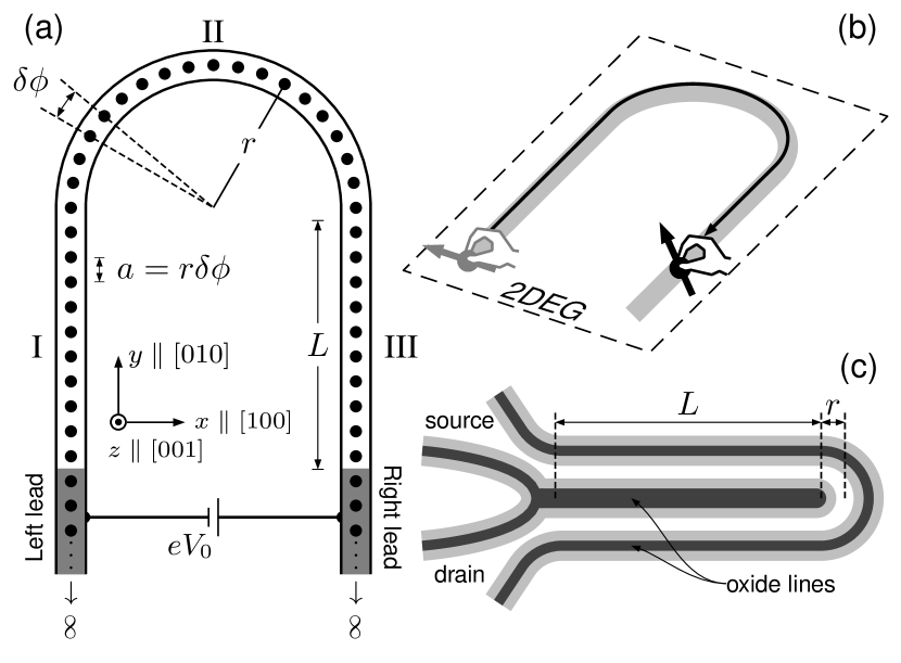
Figure 1: (a) Schematic sketch of the tight-binding model for the U-channel. Left and right arms are labeled as regions I and III, respectively, both with $N_{w}$ sites. Region II is the half-ring part with $N_{r}$ sites. (b) In quantum mechanical approaches, the electron spin propagates through the U-channel via either the translation operator or the spin propagator, which is virtually identical to dragging the spins by hand along a U-shaped path in two dimensions. (c) Schematic sketch of the U-channel realized by AFM lithography.

1D transport in QWs was previously focused on the charge properties.Ferry et al. (2009) A subsequent intensive investigation on spin-dependent transport was triggered ever since the proposal of the Datta–Das transistor,Datta and Das (1990) whose underlying mechanism is based on the Rashba spin-orbit coupling (SOC) due to structural inversion asymmetry.Bychkov1984 On the other hand, QRs provide a natural platform to study the Aharonov–Bohm effectAharonov and Bohm (1959) in solids. The idea of a “textured” magnetic field applied on the QRLoss et al. (1990) opened the study of the Berry phaseBerry (1984) in rings, in which the adiabatic transport plays a key role. The Berry phase acquired by the electron spin in rings was later discussed,Stern (1992) and investigation of the Rashba effect in QRs was subsequently initiated,Aronov and Lyanda-Geller (1993) although the employed Hamiltonian at that time was “incorrect.” After the “correct” ring version of the Rashba Hamiltonian was derived by Meijer et al. almost a decade later,Meijer et al. (2002) a series of theoretical discussion over the Rashba ring issue continued until recently.Splettstoesser et al. (2003); Frustaglia and Richter (2004); Molnár et al. (2004); Souma and Nikolić (2004); Földi et al. (2005); Wang and Vasilopoulos (2005); Földi et al. (2006)

So far we have been reviewing planar 1D systems where the curvature either vanishes (QWs) or globally exists (QRs), whereas a general 1D system may include a position dependent curvature. Quantum mechanical particle motion confined to a surface was first discussed by Jensen and KoppeJensen and Koppe (1971) and da Costa,da Costa (1981) regardless of spin, and was later generalized to include the SOC effect.Entin and Magarill (2001) When further restricted to a curved planar 1D wire, da Costa proposed a linear potential term due to curvature,da Costa (1981) which was later termed the geometric potential and has recently been observed in photonic crystals.Szameit et al. (2010)

Spin transport in a curved 1D wire in the presence of SOC was recently discussed.Trushin and Chudnovskiy (2006); Liu and Chang (2006); Zhang et al. (2007) In Ref. Trushin and Chudnovskiy, 2006, however, only the Rashba SOC was considered; in Ref. Liu and Chang, 2006, both Rashba SOC and the Dresselhaus (001) linear term (arising from the bulk inversion asymmetry of the underlying crystalDresselhaus (1955)) were taken into account, but both Refs. Trushin and Chudnovskiy, 2006 and Liu and Chang, 2006 did not consider the geometric potential. In Ref. Zhang et al., 2007, the geometric potential was considered but the SOC included only the Rashba term. Hence a more complete study of the spin transport in curved 1D wires, taking into account both Rashba and Dresselhaus terms, as well as the curvature-induced geometric potential, is essential.

Regardless of the geometric potential, spin precession due to SOCs along arbitrary paths was previously studied quantum mechanically, either through the conventional translation operatorLiu and Chang (2006) or a spin propagator obtained by a properly defined spin-orbit gauge.Chen and Chang (2008) Despite the fact that the electron spin is indeed forced to evolve through a 1D path, these spin precession studiesLiu and Chang (2006); Chen and Chang (2008) are built on a two-dimensional nature–there is no confinement. Thus how well this simple quantum mechanical picture can survive when a more realistic situation is considered, such as a lead-conductor system subject to electric bias, has for years been a question we would like to answer.

In this paper, spin precession patterns along a curved 1D wire based on the previous formalisms, namely, quantum mechanical space translation [and its approximating result spin vector formula (SVF)]Liu and Chang (2006) and spin-orbit gauge methodChen and Chang (2008) will be qualitatively and quantitatively compared with those obtained by the more sophisticated nonequilibrium Green’s function formalismDatta (1995) [or in ballistic systems free of particle-particle interaction, the Landauer–Keldysh formalism (LKF)Nikolić et al. (2005, 2006)]. Meanwhile, we will reinvestigate the influence of the geometric potential in curved 1D transport. These are regarded as our first goal. Whereas the SOCs in general depend on the momentum, electron spin traversing a curved 1D wire encounters a varying effective magnetic field. This resembles the textured magnetic fieldLoss et al. (1990) and is therefore closely related to the issue of adiabatic transport, which is our second goal in the present paper.

For these purposes we consider a U-shaped 1D channel, composed of two straight QWs and a half-QR in between, and theoretically inject electron spin from the source end and analyze the spin orientation along the U-channel down to the drain end. For computational concern, the U-channel is descretized into a finite number of lattice grid points, as sketched in Fig. 1(a). We label the left and right QWs of the U-channel as regions I and III, respectively, each containing $N_{w}$ sites, and the half-ring as region II, containing $N_{r}$ sites. In addition to the listed two goals, further investigation of the charge and spin transport properties based on the LKF will be the last goal. For the charge transport, the interplay between the Rashba and the linear Dresselhaus (001) SOCs leads to an additional modulation to the local charge density in the half-ring part of the U-channel and will be shown to originate from the emergence of the angle-dependent spin-orbit potential. For the spin transport, theoretically predicted eigenstates of the Rashba rings,Splettstoesser et al. (2003); Molnár et al. (2004); Frustaglia and Richter (2004); Földi et al. (2005); Wang and Vasilopoulos (2005) Dresselhaus rings,Wang and Vasilopoulos (2005) and the persistent spin-helix stateBernevig et al. (2006); Liu et al. (2006); Koralek et al. (2009) are numerically tested by the present quantum transport calculation.

This paper is organized as follows. In Sec. II we introduce the Hamiltonians and briefly the formalisms to be used in the transport calculations, which are reported next in Sec. III. Numerical results carrying out the above-listed three goals are reported, respectively, in Secs. III.1, III.2, and III.3. Experimental aspects regarding the fabrication of the U-channel are given in Sec. IV. We conclude in Sec. V.

II Theory

In this section we will introduce the Hamiltonians to be used in the LKF, and review the different theoretical approaches for the spin transport calculation.

II.1 Hamiltonians

In the following we first review and rederive the general form of the Hamiltonian for a continuous curved 1D system, and then apply it to the 1D ring case, which is the nontrivial part of our U-channel. We then write its corresponding tight-binding version of the Hamiltonian, to be used in the LKF calculation. Throughout we will not explicitly discuss the Hamiltonian for the straight parts of the U-channel since they are relatively trivial and well known.

II.1.1 Continuous curved 1D systems: General form

Consider the motion of electrons confined in a 1D planar curvilinear wire. Electrons originally in a two-dimensional plane are confined to a quasi-1D channel. We will derive the 1D effective Hamiltonian in the presence of SOCs. Under the effective-mass approximation in solids, the Hamiltonian for an electron in our model is

$$\mathcal{H}=\frac{\mathbf{p}^{2}}{2m}+\sum_{i=x,y}\sum_{j=x,y,z}S_{ij}p^{i}\sigma^{j}+V(\mathbf{r}),$$ (1)

where $\mathbf{p}=(p^{x},p^{y})$ is the momentum operator in two dimensions, $m$ is the effective mass, and $\sigma^{j}$’s with $j=x,y,z$ are the Pauli matrices. The second term is the general form of SOC in the Cartesian coordinate, where $S_{ij}$ is determined by SOCs linear in momentum such as Rashba or Dresselhaus (001) terms. Here $V(\mathbf{r})$ represents the potential confining electrons to the quasi-1D channel.

To obtain the effective Hamiltonian, we take the same approach as Refs. da Costa, 1981 and Zhang et al., 2007. Let $\mathbf{a}(q^{1})$ be the parametric equation of a planar curve where $q^{1}$ is the arc length of the curve. The position of an electron in the plane can be written as

$$\mathbf{r}(q^{1},q^{2})=\mathbf{a}(q^{1})+q^{2}\hat{n}(q^{1}),$$

where $\hat{n}(q^{1})$ is the unit normal vector of $\mathbf{a}(q^{1})$. $V(\mathbf{r})$ is of the form:

$$V({q^{2}})=\begin{cases}0,&q^{2}=0\\ \infty,&\text{else}\end{cases}.$$

We are going to obtain the effective 1D Hamiltonian only depending on $q^{1}$. The steps are (i) to write the Hamiltonian in the curvilinear coordinates $q^{1}$ and $q^{2}$, (ii) to write an adequate transform of wave functions and (iii) to take $q^{2}\rightarrow 0$. After these steps, the Hamiltonian will be separated into two independent parts regarding $q^{1}$ and $q^{2}$, respectively. Let $dl$ be an infinitesimal distance. We have

$$dl^{2}=g_{ij}dq^{i}dq^{j},$$

where $g_{ij}$, the metric tensor, is defined by the inner product, $(\partial\mathbf{r}/\partial q^{i})\cdot(\partial\mathbf{r}/\partial q^{j})$. We can use the coordinates $q$’s and the metric tensor $g^{ij}$ to express the Laplacian:

$$\nabla^{2}\psi=\frac{1}{\sqrt{g}}\frac{\partial}{\partial q^{i}}\left[\sqrt{g}g^{ij}\frac{\partial\psi}{\partial q^{j}}\right],$$ (2)

where $g$ is the determinant of $g_{ij}$. Once we have $S_{ij}p^{i}\sigma^{j}$ in the Cartesian coordinates, we can obtain the expression in the coordinates $q$’s via the transform’s laws of tensors:

$$\begin{split}p^{\prime i}&=\frac{\partial q^{\prime i}}{\partial q^{j}}p^{j},\\ \sigma^{\prime i}&=\frac{\partial q^{\prime i}}{\partial q^{j}}\sigma^{j},\\ S_{\mu\nu}^{{}^{\prime}}&=\frac{\partial q^{i}}{\partial q^{\prime\mu}}\frac{\partial q^{j}}{\partial q^{\prime\nu}}S_{ij},\end{split}$$ (3)

where the primed symbols denote those in the new coordinates. Using Eqs. (2) and (3), we can write the Hamiltonian of Eq. (1) in the coordinates $q$’s:

$$\mathcal{H} = -\frac{\hbar^{2}}{2m}\frac{1}{\sqrt{g}}\frac{\partial}{\partial q^{1}}\left(\sqrt{g}g^{11}\frac{\partial}{\partial q^{1}}\right)$$ (4)

$$-i\hbar\sum_{j=1}^{3}S_{1j}\sigma^{j}g^{11}\frac{\partial}{\partial q^{1}}$$

$$-\frac{\hbar^{2}}{2m}\left[\frac{\partial^{2}}{\partial{q^{2}}^{2}}+\frac{\partial}{\partial q^{2}}(\ln\sqrt{g})\frac{\partial}{\partial q^{2}}\right]$$

$$-i\hbar\sum_{j=1}^{3}S_{2j}\sigma^{j}g^{22}\frac{\partial}{\partial q^{2}}+V(q^{2}),$$

where for brevity the prime is neglected. We have used $g^{i2}=g^{2i}=\delta_{2i}$ in Eq. (4). The first two terms and latter two of Eq. (4) are not independent since $g$ is a function of $q^{1}$ and $q^{2}$. Given an eigenfunction $\Psi(q^{1},q^{2})$ of $\mathcal{H}$, we have $\mathcal{H}\Psi=E\Psi.$ Following Ref. da Costa, 1981, we make the transform $\chi(q^{1},q^{2})=f^{1/2}\Psi(q^{1},q^{2})$ with $f=\sqrt{g}=(1-\kappa q^{2})$, where $\kappa$ is the curvature of $\mathbf{a}(q^{1})$. After the transform, we obtain

$$\mathcal{H}\chi = \sqrt{f}\left[-\frac{\hbar^{2}}{2m}\frac{1}{\sqrt{g}}\frac{\partial}{\partial q^{1}}\left(\sqrt{g}g^{11}\frac{\partial}{\partial q^{1}}\frac{\chi}{\sqrt{f}}\right)\right]$$ (5)

$$-i\hbar\sum_{j=1}^{3}S_{1j}\sigma^{j}g^{11}\frac{\partial\chi}{\partial q^{1}}$$

$$-\frac{\hbar^{2}}{2m}\left\{\frac{\partial^{2}\chi}{\partial{q^{2}}^{2}}+\frac{1}{4f^{2}}\left[\left(\frac{\partial f}{\partial q^{2}}\right)^{2}\right]\chi\right\}$$

$$-i\hbar\sum_{j=1}^{3}S_{1j}\sigma^{j}g^{22}\left(\frac{\partial}{\partial q^{2}}+\frac{1}{2f}\kappa\right)\chi+V(q^{2})\chi.$$

Taking $q^{2}\rightarrow 0$ except that in $V(q^{2})$, Eq. (5) becomes

$$\mathcal{H}\chi =-\frac{\hbar^{2}}{2m}\frac{\partial^{2}\chi}{\partial{q^{1}}^{2}}-i\hbar\sum_{j=1}^{3}S_{1j}(q^{1},0)\sigma^{j}\frac{\partial\chi}{\partial q^{1}}$$

$$-\frac{\hbar^{2}}{2m}\left(\frac{\partial^{2}\chi}{\partial{q^{2}}^{2}}+\frac{\kappa^{2}\chi}{4}\right)$$

$$-i\hbar\sum_{j=1}^{3}S_{2j}(q^{1},0)\sigma^{j}\left(\frac{\partial\chi}{\partial q^{2}}+\frac{\kappa\chi}{2}\right)+V(q^{2})\chi.$$ (6)

Renaming $q^{1}$ as $s$ and deleting the terms dependent on $q^{2}$ in Eq. (6), we obtain the 1D effective Hamiltonian

$$\mathcal{H}_{1D} = -\frac{\hbar^{2}}{2m}\frac{\partial^{2}}{\partial s^{2}}-\frac{\hbar^{2}\kappa^{2}}{8m}$$ (7)

$$-i\hbar\mathbf{S}_{\parallel}(s)\cdot\vec{\sigma}\frac{\partial}{\partial s}-\frac{i\hbar\kappa}{2}\mathbf{S}_{\perp}(s)\cdot\vec{\sigma},$$

where $s$ denotes the arc length of the wire, and $\mathbf{S}_{\parallel}$ and $\mathbf{S}_{\perp}$ are defined by

$$\mathbf{S}_{\parallel}\cdot\vec{\sigma} =\sum_{j=1}^{3}S_{1j}(q^{1},0)\sigma^{j},$$ (8)

$$\mathbf{S}_{\perp}\cdot\vec{\sigma} =\sum_{j=1}^{3}S_{2j}(q^{1},0)\sigma^{j}.$$ (9)

The second term in Eq. (7) is the curvature-induced geometric potential, which was first introduced by da Costada Costa (1981) and was previously neglected in the literature of mesoscopic ring transport.Stern (1992); Aronov and Lyanda-Geller (1993); Meijer et al. (2002); Splettstoesser et al. (2003); Frustaglia and Richter (2004); Molnár et al. (2004); Souma and Nikolić (2004); Wang and Vasilopoulos (2005) We will later come back to investigate the role played by this geometric potential term.

II.1.2 1D arc with SOC: Continuous form

Below we consider the Rashba SOC in an arc. In a two-dimensional electron gas (2DEG), the intensively discussed Rashba SOCBychkov1984 reads

$$\mathcal{H}_{R}^{2D}=\frac{\alpha}{\hbar}(p^{y}\sigma^{x}-p^{x}\sigma^{y}),$$ (10)

where $\alpha$ is the Rashba coupling parameter. In this case, $S_{ij}$ are

$$\begin{split}S_{xx}&=0,\\ S_{xy}&=\frac{-\alpha}{\hbar},\\ S_{yx}&=\frac{\alpha}{\hbar},\\ S_{yy}&=0.\end{split}$$ (11)

The parametric equation for an arc can be written as $\mathbf{R}=r\hat{\rho},$ where $r$ is the radius of the ring. The position of an electron is written as $\mathbf{R}_{e}=(r-q^{2})\hat{\rho}.$ Here, $q^{1}$ is $r\phi$. Using the transform law of tensors, we obtain $S_{ij}^{\prime}$ in the $q^{i}$ coordinates from Eqs. (11), and thus

$$\begin{split}S_{11}&=0,\\ S_{12}&=\frac{-\alpha}{\hbar},\\ S_{21}&=\frac{\alpha}{\hbar},\\ S_{22}&=0.\end{split}$$ (12)

Using Eqs. (7), (8), (9), and (12), we obtain the confined $\mathcal{H}_{R}$ in the polar coordinates,

$$\mathcal{H}_{R}=-i\alpha\left(-\sigma^{2}\frac{\partial}{r\partial\phi}+\frac{\sigma^{1}}{2r}\right),$$

where $\sigma^{1}$ and $\sigma^{2}$ are defined by Eqs. (3), or in the Cartesian coordinates,

$$\mathcal{H}_{R} = -\frac{i\alpha}{r}\left(\cos\phi\sigma^{x}+\sin\phi\sigma^{y}\right)\frac{\partial}{\partial\phi}$$ (13)

$$-\frac{i\alpha}{2r}\left(\cos\phi\sigma^{y}-\sin\phi\sigma^{x}\right),$$

which is in agreement with the terms given by Meijer et al.Meijer et al. (2002)

The linear Dresselhaus (001) term, in a 2DEG expressed asDresselhaus (1955); D’yakonov and Perel (1971)

$$\mathcal{H}_{D}^{2D}=\frac{\beta}{\hbar}(p^{y}\sigma^{y}-p^{x}\sigma^{x}),$$ (14)

can be derived similarly for the arc, but can be written even more conveniently by replacing from $\mathcal{H}_{R}$ with $\alpha\rightarrow\beta,\sigma^{x}\rightarrow\sigma^{y},\sigma^{y}\rightarrow\sigma^{x}$:

$$\mathcal{H}_{D} = -\frac{i\beta}{r}\left(\cos\phi\sigma^{y}+\sin\phi\sigma^{x}\right)\frac{\partial}{\partial\phi}$$ (15)

$$-\frac{i\beta}{2r}\left(\cos\phi\sigma^{x}-\sin\phi\sigma^{y}\right).$$

Thus the 1D Hamiltonian in an arc in the presence of Rashba and linear Dresselhaus (001) SOCs reads

$$\mathcal{H}=-\frac{\hbar^{2}}{2m}\frac{\partial^{2}}{\partial s^{2}}-\frac{\hbar^{2}\kappa^{2}}{8m}+\mathcal{H}_{so},$$ (16)

where $\mathcal{H}_{so}$ is given in Eqs. (13) and (15).

II.1.3 1D arc with SOC: Tight-binding form

Previously Souma and Nikolić derived the tight-binding Hamiltonian for two-dimensional rings in the presence of Rashba SOC.Souma and Nikolić (2004) Following their construction, here we take the 1D limit, add the previously absent geometric potential term [second term in Eq. (7) or (16)] and the linear Dresselhaus (001) term, to obtain

$$H = \left(U+2t_{0}+U_{g}\right)\sigma^{0}\sum_{n}c_{n}^{{\dagger}}c_{n}$$ (17)

$$+\sum_{n}\left(\mathbf{t}_{n\leftarrow n+1}c_{n}^{{\dagger}}c_{n+1}+\text{H.c.}\right),$$

with the hopping matrix

$$\mathbf{t}_{n\leftarrow n+1} = -t_{0}\sigma^{0}+i[\cos\phi_{n,n+1}\left(t_{R}\sigma^{x}+t_{D}\sigma^{y}\right)$$ (18)

$$+\sin\phi_{n,n+1}\left(t_{R}\sigma^{y}+t_{D}\sigma^{x}\right)].$$

Here $t_{0}=\hbar^{2}/2ma^{2},$ $a$ being the lattice grid spacing, is the kinetic hopping parameter, $\sigma^{0}$ is the $2\times 2$ identity matrix, $t_{R}=\alpha/2a,t_{D}=\beta/2a$ are the Rashba and Dresselhaus hopping parameters, respectively, and $\phi_{n,n+1}=\left(\phi_{n}+\phi_{n+1}\right)/2$ is the average azimuthal angle between site $n$ and site $n+1$ ($\phi_{n+1}>\phi_{n}$; see Ref. Souma and Nikolić, 2004). In the on-site potential term in Eq. (17), $U+2t_{0}$ responsible for energy band offset corresponds to the atomic orbital energy in the language of empirical tight-binding band calculation. In general $U$ can also take into account other local potentials, but here for convenience we will put $U$ to zero. The additional term $U_{g}$ is the geometric potential and can be reexpressed in terms of $t_{0}$ as

$$U_{g}=-\frac{\hbar^{2}\kappa^{2}}{8m}=-\left(\frac{\pi}{2N_{r}}\right)^{2}t_{0},$$ (19)

where relations $\kappa=1/r$ and $N_{r}a=\pi r$ are used. Note that the $U_{g}$ term will be later considered only in the LKF, but not other quantum mechanical approaches.

II.2 Spin transport formalisms

Below we briefly review a set of different formalisms to be used to study the charge and spin transport in the U-channel. We will first introduce the tight-binding-based LKF (Sec. II.2.1), for which the U-channel is precisely described by Fig. 1(a). That is, a ferromagnetic lead is attached to the left end of the U-channel, while the right lead is made of normal metal; a bias potential difference is applied between the leads so that electrical spin injections from the left lead are theoretically simulated. Contrary to the sophisticated LKF, the quantum-mechanics-based translation (Sec. II.2.2), as well as its approximating form the SVF (Sec. II.2.3), and the spin-orbit gauge method (Sec. II.2.4) are schematically described by Fig. 1(b). That is, we simply assume an ideal spin injected at the left end of the channel, drag the spin through a U-shaped path using either a space translation operator or a more elegant spin-orbit gauge operator, and then see how the spin direction changes along the path.

II.2.1 Landauer–Keldysh formalism

The key role in the LKF is played by the lesser Green’s function, which requires (i) a tight-binding Hamiltonian and (ii) lead self-energy. For (i), the Hamiltonian matrix for the half-ring part has been introduced in Sec. II.1.3. That for the arm parts (regions I and III) can be straightforwardly constructed from the first-quantized Hamiltonians of Eqs. (10) and (14) and will not be repeated here. The size of the full Hamiltonian matrix $\left[H\right]$ amounts to $N\times N$, where $N=2N_{w}+N_{r}$ is the total number of sites. Each matrix element is a $2\times 2$ matrix because we are considering spin–$\frac{1}{2}$ systems. For (ii), we consider semi-infinite discrete leads and summarize the self-energy expression as follows.

Consider a ferromagnetic semi-infinite chain with uniform magnetization pointing along $\mathbf{e}_{M}=(\sin\theta_{M}\cos\phi_{M},\sin\theta_{M}$ $\sin\phi_{M},\cos\theta_{M})$. Extending the nonmagnetic and continuous case from Ref. Datta, 1995 to a ferromagnetic and discrete one, we obtain

$$\begin{split}\Sigma_{M}\left(E\right)&=t_{c}^{2}g_{M}^{R}\left(E\right),\\ g_{M}^{R}\left(E\right)&=\sum_{\sigma=\pm}g^{R}\left(E-\sigma t_{M}\right)|\sigma;\mathbf{e}_{M}\rangle\langle\sigma;\mathbf{e}_{M}|,\end{split}$$ (20)

where $t_{c}$ is the coupling strength between the lead and the central transport channel (and will be set equal to $t_{0}$), $t_{M}$ is the Zeeman splitting energy, the eigenkets areSakurai (1994)

$$|\sigma =+;\mathbf{e}_{M}\rangle=\left(\begin{array}[]{c}e^{-i\phi_{M}}\cos\dfrac{\theta_{M}}{2}\\ \sin\dfrac{\theta_{M}}{2}\end{array}\right),$$

$$|\sigma =-;\mathbf{e}_{M}\rangle=\left(\begin{array}[]{c}e^{-i\phi_{M}}\sin\dfrac{\theta_{M}}{2}\\ -\cos\dfrac{\theta_{M}}{2}\end{array}\right),$$

and the retarded surface Green’s function reads

$$g^{R}\left(E\right) =\frac{1}{2t_{d}}\begin{cases}\Delta-i\sqrt{4-\Delta^{2}},&\left|\Delta\right|\leq 2\\ \Delta-\mathop{\mathrm{s}gn}\Delta\sqrt{\Delta^{2}-4},&\left|\Delta\right|>2\end{cases},$$

$$\Delta =\frac{E-\left(V+2t_{d}\right)}{t_{d}},$$

where $t_{d}$ is the kinetic hopping parameter in the lead and will be again set equal to $t_{0}$ in the later computation. The self-energy function, Eq. (20), is the only nonvanishing matrix element of the full self-energy matrices: $\left[\Sigma_{L}(E)\right]_{11}$ and $\left[\Sigma_{R}(E)\right]_{NN}$. For our U-channel here, we will consider for the left lead $t_{M}=0.1t_{0}$ to inject spins while for the right lead $t_{M}=0$ to let the spins outflow freely.

With both the tight-binding Hamiltonian and lead self-energy matrix constructed, one can construct the space-resolved retarded Green’s function matrix

$$\left[G^{R}\left(E\right)\right]=\left\{E\left[I\right]-\left[H\right]-\left[\Sigma_{L}\left(E\right)\right]-\left[\Sigma_{R}\left(E\right)\right]\right\}^{-1},$$

where $\left[I\right]$ is the $2N\times 2N$ identity matrix, $\left[H\right]$ is the space-resolved tight-binding Hamiltonian matrix for the U-channel, and $\left[\Sigma_{L/R}\left(E\right)\right]$ is the self-energy matrix of the left/right lead. The lesser Green’s function matrix is then obtained via the kinetic equation

$$\left[G^{<}\left(E\right)\right]=\left[G^{R}\left(E\right)\right]\left[\Sigma^{<}\left(E\right)\right]\left[G^{A}\left(E\right)\right],$$ (21)

where $\left[G^{A}\left(E\right)\right]$ is the advanced Green’s function matrix obtained by the Hermitian conjugate of $\left[G^{R}\left(E\right)\right]$ and the lesser self-energy matrix is given by

$$\left[\Sigma^{<}\left(E\right)\right] = -\sum_{p=L,R}\left\{\left[\Sigma_{p}\left(E-eV_{p}\right)\right]-\left[\Sigma_{p}\left(E-eV_{p}\right)\right]^{{\dagger}}\right\}$$

$$\times f_{0}\left(E-eV_{p}\right),$$

where $f_{0}$ is the Fermi function and $eV_{p}$ is the electric potential energy applied on lead $p$. In our numerical computation we will put $eV_{L}=+eV_{0}/2$ and $eV_{R}=-eV_{0}/2$ for a potential energy difference of $eV_{0}$, a bias parameter that is taken as positive (while the electron charge $e=-\left|e\right|$ is negative), so that the electrons are injected from the left lead. In addition, we will consider a zero-temperature limit so that the Fermi function becomes step-like and will strictly cut the energy integration range [see Eqs. (22) and (23) below].

Desired physical quantities can then be extracted from the lesser Green’s function, Eq. (21), through properly defined expressions.Nikolić et al. (2006) In this paper our main interest lies in the local charge density,

$$e\langle N_{n}\rangle=\frac{e}{2\pi i}\int_{E_{F}-eV_{0}/2}^{E_{F}+eV_{0}/2}dE\mathop{\mathrm{T}r}_{s}\left[G^{<}\left(E\right)\right]_{nn},$$ (22)

and the local spin density,

$$\begin{split}\langle S_{n}^{i}\rangle=&\frac{\hbar/2}{2\pi i}\int_{E_{F}-eV_{0}/2}^{E_{F}+eV_{0}/2}dE\mathop{\mathrm{T}r}_{s}\left\{\sigma^{i}\left[G^{<}\left(E\right)\right]_{nn}\right\},\\ i=&x,y,z\end{split}$$ (23)

where $E_{F}$ is the Fermi level that will be set to $0.2t_{0}$ above the band bottom, $\left[G^{<}\left(E\right)\right]_{nn}$ is the $n$th diagonal matrix element of the entire $\left[G^{<}\left(E\right)\right]$ matrix and is a $2\times 2$ matrix, and $\mathop{\mathrm{T}r}_{s}$ is the trace done with respect to spin. The subscript on the left-hand sides of both Eqs. (22) and (23) stand for the $n$th site of the U-channel.

II.2.2 Quantum mechanical translation method

In the following we briefly review an earlier work done by some of us,Liu and Chang (2006) a theoretical method based on quantum mechanics to analyze spin precession along an arbitrary path.

An electron spin injected at $\mathbf{r}_{0}$ is described by a state ket $|\mathbf{s}_{0};\mathbf{r}_{0}\rangle,$ where $\mathbf{s}_{0}$ labels the spin orientation, and is later evolved to another state ket $|\mathbf{s};\mathbf{r}\rangle$ at position $\mathbf{r}$, through the translation operator $\mathcal{T}\left(\mathbf{p}\right)=\exp\left[i\mathbf{p}/\hbar\cdot\left(\mathbf{r}-\mathbf{r}_{0}\right)\right]$, i.e., $|\mathbf{s};\mathbf{r}\rangle=\mathcal{T}\left(\mathbf{p}\right)|\mathbf{s}_{0};\mathbf{r}_{0}\rangle$. In two-dimensional boundless systems with Rashba and linear Dresselhaus (001) SOCs [Eqs. (10) and (14)], the eigenstates $|\pm;\phi_{k}\rangle$ are well known (see, for example, also Ref. Liu and Chang, 2006) and can serve as a convenient basis to expand the spin state ket; $\phi_{k}$ is the propagation angle of wave vectors $\mathbf{k}_{\pm}$. Hence, expanding $|\mathbf{s}_{0};\mathbf{r}_{0}\rangle$ in terms of $|\pm;\phi_{k}\rangle$, we can proceed by using $f\left(\mathbf{p}\right)|\pm;\phi_{k}\rangle=f\left(\hbar\mathbf{k}_{\pm}\right)|\pm;\phi_{k}\rangle$:

$$|\mathbf{s};\mathbf{r}\rangle = \mathcal{T}\left(\mathbf{p}\right)|\mathbf{s}_{0};\mathbf{r}_{0}\rangle$$ (24)

$$= e^{i\mathbf{k}_{\pm}\cdot\left(\mathbf{r}-\mathbf{r}_{0}\right)}\sum_{\sigma=\pm}|\sigma;\phi_{k}\rangle\langle\sigma;\phi_{k}|\mathbf{s}_{0};\mathbf{r}_{0}\rangle$$

$$= e^{i\bar{k}\Delta r}\sum_{\sigma=\pm}e^{i\sigma\Delta\theta/2}|\sigma;\phi_{k}\rangle\langle\sigma;\phi_{k}|\mathbf{s}_{0};\mathbf{r}_{0}\rangle,$$

with $\bar{k}=(k_{+}+k_{-})/2,\Delta\theta=\Delta k\Delta r=(k_{+}-k_{-})\Delta r,$ and $\Delta r=\left|\mathbf{r}-\mathbf{r}_{0}\right|$. The global phase involving $\bar{k}$ will be canceled in calculating the expectation value while the phase difference involving $\Delta k=-2m\zeta/\hbar^{2}$ with $\zeta$ given later in Eq. (29) plays a key role in spin precession. For successive nearest-neighbor hoppings in Fig. 1(a), we simply apply Eq. (24) for every step and then calculate the expectation value for Pauli matrices to obtain the spin direction on each site, $\langle\mathbf{S}\rangle=(\hbar/2)\langle\vec{\sigma}\rangle=(\hbar/2)\langle\mathbf{s};\mathbf{r}|(\sigma_{x},\sigma_{y},\sigma_{z})|\mathbf{s};\mathbf{r}\rangle,$ starting with the assumed injected spin at the first site in contact with the left lead.

II.2.3 Spin vector formula

A further approximating step done in Ref. Liu and Chang, 2006 (see the Appendix therein) was to take the continuous limit, so that each section approaches to infinitesimal. After successive infinitesimal translations from injection point $\mathbf{r}_{0}$ to a certain desired position $\mathbf{r}$, the spinor overlaps carried by the final state ket were approximated as

$$\langle\sigma_{1}|\sigma_{0}\rangle\langle\sigma_{2}|\sigma_{1}\rangle\cdots\langle\sigma_{j+1}|\sigma_{j}\rangle\cdots\langle\sigma_{N}|\sigma_{N-1}\rangle$$ (25)

$$\approx \langle\sigma_{1}|\sigma_{0}\rangle\delta_{\sigma_{2}\sigma_{1}}\cdots\delta_{\sigma_{j+1}\sigma_{j}}\cdots\delta_{\sigma_{N}\sigma_{N-1}},$$

where $|\sigma_{0}\rangle=|\mathbf{s}_{0};\mathbf{r}_{0}\rangle$ is the input, $|\sigma_{j}\rangle$ is the shorthand for $|\sigma_{j};\phi_{k}^{j}\rangle$, $\phi_{k}^{j}$ being the propagation angle of the $j$th section, and $N\rightarrow\infty$ is the number of infinitesimal straight translations from $\mathbf{r}_{0}$ to $\mathbf{r}$. A closed form of the state ket generalized from Eq. (24) can thus be obtained. Using the generalized state ket one obtains the SVF,

$$\langle\mathbf{S}\rangle=\frac{\hbar}{2}\left(\begin{array}[]{c}-\cos\theta_{M}\cos\varphi_{k}\sin\Delta\Theta+\sin\theta_{M}\left[\cos\left(\varphi_{k}-\varphi_{k}^{0}+\phi_{M}\right)\cos^{2}\dfrac{\Delta\Theta}{2}-\cos\left(\varphi_{k}+\varphi_{k}^{0}-\phi_{M}\right)\sin^{2}\dfrac{\Delta\Theta}{2}\right]\\ -\cos\theta_{M}\sin\varphi_{k}\sin\Delta\Theta+\sin\theta_{M}\left[\sin\left(\varphi_{k}-\varphi_{k}^{0}+\phi_{M}\right)\cos^{2}\dfrac{\Delta\Theta}{2}-\sin\left(\varphi_{k}+\varphi_{k}^{0}-\phi_{M}\right)\sin^{2}\dfrac{\Delta\Theta}{2}\right]\\ \cos\theta_{M}\cos\Delta\Theta+\sin\theta_{M}\cos\left(\varphi_{k}^{0}-\phi_{M}\right)\sin\Delta\Theta\end{array}\right),$$ (26)

with

$$\varphi_{k}=\arg[(\alpha\cos\phi_{k}-\beta\sin\phi_{k})+i(\alpha\sin\phi_{k}-\beta\cos\phi_{k})],$$ (27)

$$\Delta\Theta=\frac{2m^{\star}}{\hbar^{2}}\int_{C}\zeta ds,$$ (28)

$$\zeta=\sqrt{\alpha^{2}+\beta^{2}-2\alpha\beta\sin 2\phi_{k}\left(s\right)}.$$ (29)

The angle $\varphi_{k}^{0}$ in Eq. (26) stands for $\varphi_{k}\left(\phi_{k}^{0}\right),$ where $\phi_{k}^{0}$ is the propagation direction of the input $|\mathbf{s}_{0};\mathbf{r}_{0}\rangle$.

For the present U-channel, the transport direction as a function of position coordinate $s$ can be written as

$$\phi_{k}\left(s\right)=\begin{cases}\pi/2,&s\in\left[0,L\right]\\ \pi/2-\pi\frac{s-L}{\pi r},&s\in\left[L,L+\pi r\right]\\ -\pi/2,&s\in[L+\pi r,2L+\pi r]\end{cases},$$ (30)

$L$ being the length of each arm; $s$ runs from $0$ to $2L+\pi r$. In the following we give two concrete examples to show the convenience of Eq. (26), one for the pure Rashba case and the other for the pure Dresselhaus, both with $S^{x}$ spin injection: $(\theta_{M},\phi_{M})=(\pi/2,0)$.

In the presence of only the Rashba SOC, we have from Eq. (27) $\varphi_{k}^{0}=\phi_{k}\left(s=0\right)=\pi/2,$ $\varphi_{k}=\phi_{k}\left(s\right)$ and from Eqs. (28) and (29) $\Delta\Theta=2(t_{R}/t_{0})(s/a)$. Putting these together with $(\theta_{M},\phi_{M})=(\pi/2,0)$ into Eq. (26) we have

$$\left.\langle\mathbf{S}\rangle\right|_{R,S^{x}\text{ inj}}=\frac{\hbar}{2}\left(\begin{array}[]{c}\sin\phi_{k}\\ -\cos\phi_{k}\\ 0\end{array}\right).$$ (31)

In the presence of only the linear Dresselhaus (001) SOC, we have $\varphi_{k}^{0}=-\pi,\varphi_{k}=-\phi_{k}(s)-\pi/2,$ and $\Delta\Theta=2(t_{D}/t_{0})(s/a)$. Equation (26) then reduces to

$$\left.\langle\mathbf{S}\rangle\right|_{D,S^{x}\text{ inj}}=\frac{\hbar}{2}\left(\begin{array}[]{c}\cos\Delta\Theta\sin\phi_{k}\\ \cos\Delta\Theta\cos\phi_{k}\\ -\sin\Delta\Theta\end{array}\right).$$ (32)

Despite the elegant description of these SVFs, a crucial approximation of the spinor overlaps that has been made in Eq. (25) deserves a further discussion before we move on. Take one pair of the overlap, say, between $j$th and $(j+1)$th. Recall the eigenspinors in the presence of both Rashba and linear Dresselhaus (001) SOCs,Liu and Chang (2006)

$$|\sigma_{j}\rangle=\frac{1}{\sqrt{2}}\left(\begin{array}[]{c}ie^{-i\varphi_{k}^{j}}\\ \sigma_{j}\end{array}\right),$$ (33)

where $\varphi_{k}^{j}=\varphi_{k}(\phi_{k}^{j})$ is given in Eq. (27). When the two sections point along the same direction, i.e., $\phi_{k}^{j}=\phi_{k}^{j+1}$, the orthogonality becomes exact: $\langle\sigma_{j+1}|\sigma_{j}\rangle=\delta_{\sigma_{j+1}\sigma_{j}}$, regardless of the type of the SOCs in the straight 1D structure. Otherwise, the orthogonal approximation always contains an error. For the pure Rashba case, the overlap using Eq. (33) up to first order in $\Delta\phi_{k}$ reads $\langle\sigma_{j+1}|\sigma_{j}\rangle=(e^{i(\phi_{k}^{j+1}-\phi_{k}^{j})}+\sigma_{j+1}\sigma_{j})/2=\delta_{\sigma_{j+1}\sigma_{j}}+i\Delta\phi_{k}/2+\cdots,$ which indicates that the major error term accumulating upon “turning” along the curved 1D structure is proportional to the change of the angle $\Delta\phi_{k}=\phi_{k}^{j+1}-\phi_{k}^{j}$ and is therefore still moderate. In the presence of only the linear Dresselhaus term, the situation is similar. In the presence of both SOC terms, however, the error accumulated becomes drastic, which we will show numerically later.

II.2.4 Spin-orbit gauge method

The spin propagator can be obtained with the help of a spin-orbit gauge.Chen and Chang (2008) Noting that the highest order in momentum $\mathbf{P}=\mathbf{p}\sigma^{0}$ in the Hamiltonian of a 2DEG with Rashba and Dresselhaus SOCs (both linear in $\mathbf{p}$) is quadratic, one can define the spin-orbit gauge,

$$\mathbf{A}^{\text{SO}}=\left(A_{x},A_{y}\right)\equiv\frac{mc}{e\hbar}\left(\alpha\sigma_{y}+\beta\sigma_{x},-\alpha\sigma_{x}-\beta\sigma_{y}\right),$$ (34)

to express the 2DEG Hamiltonian,

$$\mathcal{H}^{RD} = \frac{\mathbf{P}^{2}}{2m}+\mathcal{H}_{R}^{2D}+\mathcal{H}_{D}^{2D}$$ (35)

$$= \frac{1}{2m}\left(\mathbf{P-}\frac{e}{c}\mathbf{A}^{\text{SO}}\right)^{2}-V_{b}\sigma^{0}$$

with the constant background potential $V_{b}=(m/\hbar^{2})\left(\alpha^{2}+\beta^{2}\right)$; recall that $\sigma^{0}$ is the $2\times 2$ identity matrix. Consider now the transformation operator,

$$\mathcal{U}^{\text{SO}}\left(\mathbf{r}\right)=\exp\left[\frac{ie}{\hbar c}\left(\mathbf{A}^{\text{SO}}\cdot\mathbf{r}\right)\right],$$ (36)

with the unitary property $\mathcal{U}^{\text{SO}}\left(\mathbf{r}\right)\mathcal{U}^{\text{SO}}\left(\mathbf{r}\right)^{{\dagger}}=\sigma^{0}$ ensured by the Hermitian $\mathbf{A}^{\text{SO}}=\mathbf{A}^{\text{SO}{\dagger}}$ from definition (34) and $\mathbf{r}$ being the position vector of the electron displacement. Since the spin-orbit-interacting Hamiltonian of Eq.  (35) differs from the Hamiltonian of the free electron gas (with a background potential $V_{b}$),

$$\mathcal{H}^{\text{free}}=\frac{\mathbf{P}^{2}}{2m}-V_{b}\sigma^{0}\text{,}$$ (37)

only by the gauge term $(e/c)\mathbf{A}^{\text{SO}}$ in $\mathbf{P}$, the following transformation is therefore suggested:

$$\mathcal{U}^{\text{SO}}\left(\mathbf{r}\right)\mathbf{P}\mathcal{U}^{\text{SO}}\left(\mathbf{r}\right)^{{\dagger}}=\mathbf{P+}\frac{ie}{\hbar c}\left[\mathbf{A}^{\text{SO}}\cdot\mathbf{r,P}\right]$$

$$+\frac{1}{2}\left(\frac{ie}{\hbar c}\right)^{2}\left[\mathbf{A}^{\text{SO}}\cdot\mathbf{r,}\left[\mathbf{A}^{\text{SO}}\cdot\mathbf{r,P}\right]\right]+\cdots,$$ (38)

with $[\mathbf{A}^{\text{SO}}\cdot\mathbf{r},\mathbf{P]}=i\hbar\mathbf{A}^{\text{SO}}$. Due to the noncommutability $[A_{x}^{\text{SO}},A_{y}^{\text{SO}}]\neq 0$, the terms containing higher orders of $\left|\mathbf{r}\right|$, in general, do not vanish, while in the small-displacement limit $\left|\mathbf{r}\right|\approx 0$ in which one has $e\left(c\hbar\right)^{-1}\mathbf{A}^{\text{SO}}\cdot\mathbf{r}\ll 1$, Eq. (38) reduces to $\mathcal{U}^{\text{SO}}\left(\mathbf{r}\right)\mathbf{P}\mathcal{U}^{\text{SO}}\left(\mathbf{r}\right)^{{\dagger}}=\mathbf{P-}e/c\mathbf{A}^{\text{SO}}$, rendering the following transformation,

$$\mathcal{U}^{\text{SO}}\left(\mathbf{r}\right)\mathcal{H}^{\text{free}}\mathcal{U}^{\text{SO}}\left(\mathbf{r}\right)^{{\dagger}}=\mathcal{H}^{RD}\text{,}$$ (39)

between the two systems, $\mathcal{H}^{RD}$ and $\mathcal{H}^{\text{free}}$. Accordingly, when $\left|\mathbf{r}\right|\approx 0$ or $e\left(c\hbar\right)^{-1}\mathbf{A}^{\text{SO}}\cdot\mathbf{r}\ll 1$ is satisfied, the free electron gas $\mathcal{H}^{\text{free}}$, Eq. (37), and the spin-orbit-interacting electron gas $\mathcal{H}^{RD}$, Eq. (35), share the same eigenenergies $E_{\mathbf{k}}$. Their corresponding eigenfunctions, denoted by $\psi_{E_{\mathbf{k}}}(\mathbf{r)}\chi_{s}^{\text{free}}$ and $\Psi_{E_{\mathbf{k}}}(\mathbf{r)}\chi_{s}^{\text{SO}}$, respectively, differ from each other only by a phase factor, the $2\times 2$ matrix $\mathcal{U}^{\text{SO}}\left(\mathbf{r}\right)$, namely, $\Psi_{E_{\mathbf{k}}}(\mathbf{r)}\chi_{s}^{\text{SO}}=$ $\psi_{E_{\mathbf{k}}}(\mathbf{r)}\mathcal{U}^{\text{SO}}\left(\mathbf{r}\right)\chi_{s}^{\text{free}}$. Here $\chi_{s}$ is the spin part of the wave function. Moreover, any wave function is constructed by a superposition of the eigenfunctions, so for any given wave function $\psi(\mathbf{r)}\chi_{s}^{\text{free}}$ in $\mathcal{H}^{\text{free}}$, the corresponding wave function in $\mathcal{H}^{RD}$ is $\psi(\mathbf{r)}\mathcal{U}^{\text{SO}}\left(\mathbf{r}\right)\chi_{s}^{\text{free}}$.

The correspondence, which originated from gauge transformation (39), between $\mathcal{H}^{\text{free}}$ and $\mathcal{H}^{RD}$ systems, allows one to construct the spin propagator for $\mathcal{H}^{RD}$; to elaborate on this, consider an injected electron in system $\mathcal{H}^{\text{free}}$ described by $\psi_{\text{inj}}(\mathbf{r)}\chi_{\text{inj}}=[\sum_{{}_{\mathbf{k}}}C_{\mathbf{k}}\psi_{E_{\mathbf{k}}}(\mathbf{r)]}\chi_{\text{inj}}$ with the initial spin state $\chi_{\text{inj}}$ and the weighting factor $C_{\mathbf{k}}$. Without any spin-dependent mechanisms, this electron remains at spin state $\chi_{\text{inj}}$, while importing $\mathbf{A}^{\text{SO}}$ turns on $\mathcal{U}^{\text{SO}}\left(\mathbf{r}\right)$ so that the electron wave function in the spin-orbit-interacting system $\mathcal{H}^{RD}$ can be expressed by the gauge transformation in the form,

$$\mathcal{U}^{\text{SO}}\left(\mathbf{r}\right)\psi_{\text{inj}}\left(\mathbf{r}\right)\chi_{\text{inj}}=\sum_{\mathbf{k}}C_{\mathbf{k}}\psi_{E_{\mathbf{k}}}\left(\mathbf{r}\right)\mathcal{U}^{\text{SO}}\left(\mathbf{r}\right)\chi_{\text{inj}}\text{.}$$ (40)

As a result, the spin polarization of the electron in system $\mathcal{H}^{RD}$ varies spatially according to $\mathcal{U}^{\text{SO}}\left(\mathbf{r}\right)\chi_{\text{inj}}$, and thus $\mathcal{U}^{\text{SO}}\left(\mathbf{r}\right)$ can be viewed as a spin propagator.

For general applications based on the gauge transformation, assume an electron moving along an arbitrarily curved trajectory denoted as path $c$ starting from one spatial point to the other. Divide this path into $N$ pieces. Label the divided pieces (paths) by path $1$, path $2$, $\ldots$, path $N$, sequentially (i.e., path $i+1$ follows path $i$), and let $\mathbf{r}_{i}$ denote the position vector of the displacement for the $i$th path. One can always choose large-enough $N$ to have $e\left(c\hbar\right)^{-1}\mathbf{A}^{\text{SO}}\cdot\mathbf{r}_{i}\ll 1$ such that Eq. (36) can be approximately interpreted as a propagator for each $\mathbf{r}_{i}$. The spin propagator along an arbitrary path $c$ then reads

$$\mathcal{U}_{c}^{\text{SO}}\left(\mathbf{r}\right)=\mathcal{U}^{\text{SO}}\left(\mathbf{r}_{N}\right)\mathcal{U}^{\text{SO}}\left(\mathbf{r}_{N-1}\right)\cdots\mathcal{U}^{\text{SO}}\left(\mathbf{r}_{2}\right)\mathcal{U}^{\text{SO}}\left(\mathbf{r}_{1}\right)\text{,}$$ (41)

which can be concisely written as

$$\mathcal{U}_{c}^{\text{SO}}\left(\mathbf{r}\right)=\mathcal{P}\exp\left(\frac{ie}{\hbar c}\int_{c}\mathbf{A}^{\text{SO}}\cdot d\mathbf{r}\right)\text{,}$$ (42)

where $\mathcal{P}$ is the path-ordering operator that orders the operator $\mathcal{U}^{\text{SO}}\left(\mathbf{r}_{i}\right)$ with earlier passing path $\mathbf{r}_{i}$ to the right of the later $\mathcal{U}^{\text{SO}}\left(\mathbf{r}_{i+1}\right)$ such that $\mathcal{P}\exp[(ie/\hbar c)\int_{\text{path }i+1\leftarrow\text{path }i}\mathbf{A}^{\text{SO}}\cdot d\mathbf{r}]=\mathcal{U}^{\text{SO}}\left(\mathbf{r}_{i+1}\right)\mathcal{U}^{\text{SO}}\left(\mathbf{r}_{i}\right)$.

Obviously, if both the $i$th and $(i+1)$th paths form a straight line, then one has

$$\mathcal{U}^{\text{SO}}\left(\mathbf{r}_{i+1}+\mathbf{r}_{i}\right)=\mathcal{U}^{\text{SO}}\left(\mathbf{r}_{i+1}\right)\mathcal{U}^{\text{SO}}\left(\mathbf{r}_{i}\right)$$ (43)

simply because only one dimension (component) of $\mathbf{A}^{\text{SO}}$ will be used, and thus the commutators that appeared in the higher-order terms of Eq. (38) vanish. In other words, if the electron moves along a straight line, i.e., path $c$ is not curved, we have $\mathcal{U}_{c}^{\text{SO}}\left(\mathbf{r}\right)=\mathcal{U}^{\text{SO}}\left(\mathbf{r}\right)$, namely, Eq. (42) reduces to Eq. (36).

To study the spin evolution through the U-channel in the continuous limit, one can use $\mathcal{U}^{\text{SO}}\left(\mathbf{r}\right)$ for parts I and III and Eq. (41) for part II. To be consistent with the discrete tight-binding model shown in Fig. 1(a) adopted in the LKF, however, we will successively apply $\mathcal{U}^{\text{SO}}\left(\mathbf{r}\right)$ for each nearest-neighbor hopping.

III Transport analysis

Having reviewed the theoretical formalisms, we are now in a position to carry out our three goals of this paper. In Sec. III.1, we compare the spin precession patterns calculated by quantum mechanical approaches with those by the LKF, or nowadays generally termed quantum transport. Meanwhile, we will examine the role played by the curvature-induced geometric potential based on the LKF. We proceed in Sec. III.2 with a detailed discussion for adiabatic and nonadiabatic transport regimes and connect the present paper with previous ones. In Sec. III.3 we discuss the anisotropic charge transport due to the interplay between the Rashba and Dresselhaus SOCs, and spin precession in special cases, which is equivalent to numerically testing the eigenstates of Rashba rings, Dresselhaus rings, and the persistent spin-helix state.

III.1 Quantum mechanical approaches vs quantum transport

III.1.1 Weak geometric potential

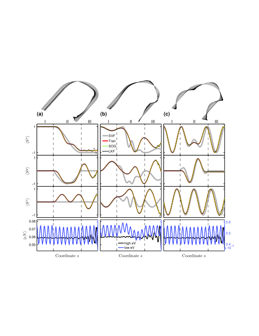
Figure 2: (Color online) Spatially resolved spin components (in units of $\hbar/2$) calculated by the LKF, translation method (Tran), spin-orbit gauge (SOG) method, and SVF in a U-channel with $(N_{w},N_{r})=(30,50)$ under a strong bias of $eV_{0}=0.4t_{0}$ and SOC strengths of (a) $(t_{R},t_{D})=(0.1,0)t_{0}$, (b) $(t_{R},t_{D})=(0.1,0.03)t_{0}$, and (c) $(t_{R},t_{D})=(0,0.1)t_{0}.$ The local charge densities obtained by the LKF for a high bias of $eV_{0}=0.4t_{0}$ and low bias of $eV_{0}=10^{-3}t_{0}$ are shown in the bottom panels. Spin vectors in the top subplots are based on the high-bias LKF results.

Recall the geometric potential $U_{g}$ expressed in terms of $t_{0}$ in Eq. (19). From the tight-binding Hamiltonian of Eq.  (17), one can see that whether $U_{g}$ is sensible by the electrons depends on its competition with the energy band width $2t_{0}$. Here we begin with a U-channel with $N_{r}=50,$ yielding $\left|U_{g}\right|\approx 2.47\times 10^{-4}t_{0},$ which is hardly competitive with $2t_{0}$, and $N_{w}=30$.

In Fig. 2 we report the local spin densities calculated by the LKF under a high bias of $eV_{0}=0.4t_{0}$, spin components by the SVF, translation method, and spin-orbit gauge method, for the pure Rashba case with $t_{R}=0.1t_{0}$ in column (a), pure Dresselhaus case with $t_{D}=0.1t_{0}$ in column (c), and a mixed case with $(t_{R},t_{D})=(0.1,0.03)t_{0}$ in column (b). At the bottom of each column, the local charge density obtained by the LKF with both a high bias of $eV_{0}=0.4t_{0}$ and a low bias of $eV_{0}=10^{-3}t_{0}$ is also reported. At the top of each column, the spatially imaged spin vectors are from the LKF results. Note that the LKF-based spin densities $\langle S_{n}^{i}\rangle$ given by Eq. (23) have been normalized by requiring $\left|\langle\mathbf{S}_{n=1}\rangle\right|=\hbar/2$, while the spin components obtained by the quantum mechanical methods are inherently of unit norm due to the normalized state kets.

Clearly in Fig. 2 all the spin curves obtained by translation and by spin-orbit gauge methods are identical to each other. These curves further fit with those obtained by the LKF all quite well, except the oscillating tails that appear in the LKF results. These oscillations result from the nonequilibrium accumulation of the electron number that cannot be taken into account in the quantum mechanical approaches. With low bias the electrons behave like waves (as shown in the charge density curves in the bottom panels of Fig. 2), which is the assumption in the quantum mechanical approaches. The spin density curves obtained by translation or spin-orbit gauge method match those obtained by the LKF with low bias perfectly (not shown).

For the curves from SVFs, we use Eq. (31) for the Rashba case of Fig. 2(a), Eq. (32) for the Dresselhaus case of Fig. 2(c), and Eq. (26) for the mixed case of Fig. 2(b). In region I of all three cases, the SVF curves match all the others perfectly since in that region the orthogonality approximation Eq. (25) is in fact exact. Once the electron enters region II, the error contained in Eq. (25) for the SVF curves starts to accumulate. The error is still moderate in Figs. 2(a) and 2(c), but becomes drastic in the mixed case of Fig. 2(b), as we have remarked previously in Sec. II.2.3.

Comparing the low-bias charge densities in all three cases, one can see that an additional modulation appears in region II when both SOCs are present [bottom panel of Fig.  2(b)]. This charge density modulation stems from the angle-dependent spin-orbit potential, and will be explained in detail later in Sec. III.3.1.

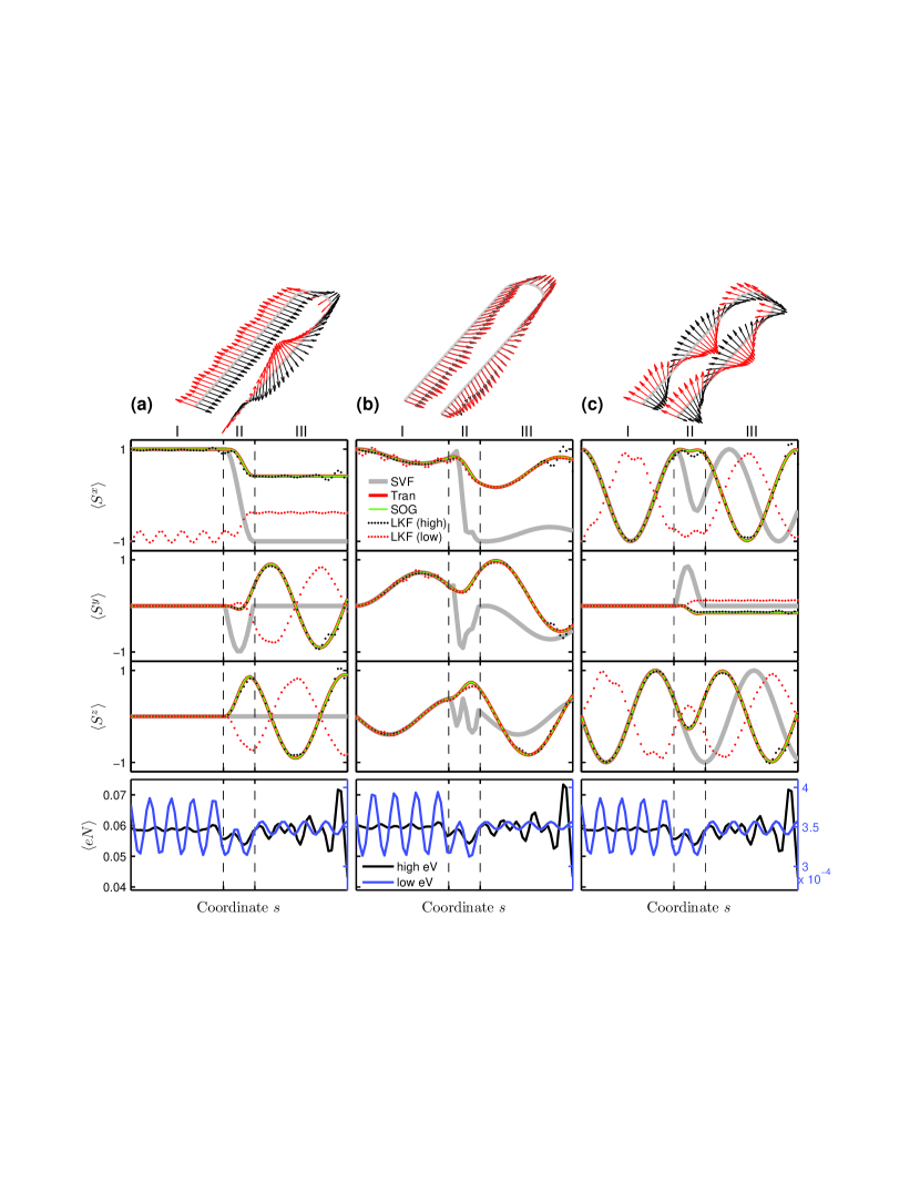
Figure 3: (Color online) Similar to Fig. 2 but $N_{r}=10$. Spin densities obtained by the LKF are shown for both low and high bias. In the top subplots, black or red (gray) vectors correspond to high- or low-bias LKF calculations.

Before leaving for the stronger geometric potential case, we give a further discussion over the Rashba channel: Fig. 2(a). Since $S^{x}$ is one of the Rashba eigenstates in region I, the injected spin perfectly retains its spin direction until the half-ring section is reached. Then nonvanishing $\langle S^{z}\rangle$ component is induced in the curves from the LKF, and translation or spin-orbit gauge method since the eigenstates of the Rashba ring are no longer in-plane.Splettstoesser et al. (2003); Molnár et al. (2004); Frustaglia and Richter (2004) The spin direction described by the SVF, on the other hand, remains in-plane and perpendicular to the transport, since after the orthogonal approximation [Eq. (25)] the coplanar normal of a continuous 1D channel is still concluded as the eigenstate. Hence the “generalized precessionless” transport in the curved 1D Rashba channel predicted in Ref. Liu and Chang, 2006 may not work well. The $S^{x}$ spin entering the half-ring region, in fact, starts to precess about the tilted eigenstate of the Rashba ring with spin precession length $L_{so}$ [given later in Eq. (45)], which matches exactly the period shown in $\langle S^{z}\rangle$ of Fig. 2(a). We will come back to this tilted eigenstate later in Sec. III.3.2.

III.1.2 Strong geometric potential

Next we consider a U-channel with $N_{r}=10$ and the same $N_{w}$. The geometric potential for such a $N_{r}$ is $\left|U_{g}\right|=0.025t_{0},$ which is no longer negligible for the electrons. We keep the same figure orientation as Fig. 2. The only information added in Fig. 3 is the spin components computed by the LKF with low bias.

The spin curves by translation and spin-orbit gauge methods are again identical to each other and match the LKF curves with high bias well. SVF curves this time become rather poor after entering the half-ring region since there the change in the direction $\Delta\phi_{k}$ upon every hopping is no longer small and the spinor overlap approximation (25) hardly applies.

For the spin curves obtained by the LKF with low bias, the effect of the geometric potential $U_{g}$ can now be seen. The injected spin previously parallel to the internal magnetic field direction $\mathbf{e}_{M}$ is here reversed due to the reflection off the $U_{g}$ potential well and a certain matching condition between the Fermi wavelength and the arm length $L$ within region I. Shifting the Fermi energy $E_{F}$, changing the length $L$, or putting different SOC energies [such as Fig. 3(b)] will make the reversal of the spin direction disappear. This is also why, in the strong-bias regime, where a larger range of contributing states are integrated, the reversal does not show.

The huge difference due to the stronger $U_{g}$ shown in Fig. 3 is hence only a special case: The reflection off the $U_{g}$ well and the length matching happen to make the opposite spin state favored upon injection. Here we conclude that the role played by the geometric potential is merely a rather weak potential well that can be possibly sensed by the electrons when the bending of the 1D structure is severe, and that even if $U_{g}$ is sensed, it serves simply as a potential well, which becomes crucial only in the linear transport regime with a certain particular matching condition between the Fermi wavelength and the channel size.

Apart from the spin behavior, the potential well nature of the $U_{g}$ can be clearly identified by comparing the low-bias charge density curves shown in the bottom panels of Figs. 2 and 3. In the previous weak $U_{g}$ case, the electron density distributes like a standing wave from the source to the drain ends, while in the present strong $U_{g}$ case the electron wave is disturbed by the central geometric potential well in the half-ring part.

III.2 Adiabatic and nonadiabatic transport regimes

Comparing further the previous two U-channels, one can see from the Rashba cases that the spin initially injected at one of the Rashba wire eigenstates may or may not follow the local eigenstate throughout the U-channel; see Fig. 4(a). Certainly the key lies on the half-ring part, where the larger the number $N_{r}$ is, the easier the spin can follow the eigenstate, but the strength of the SOC is also an important factor.Frustaglia and Richter (2004)

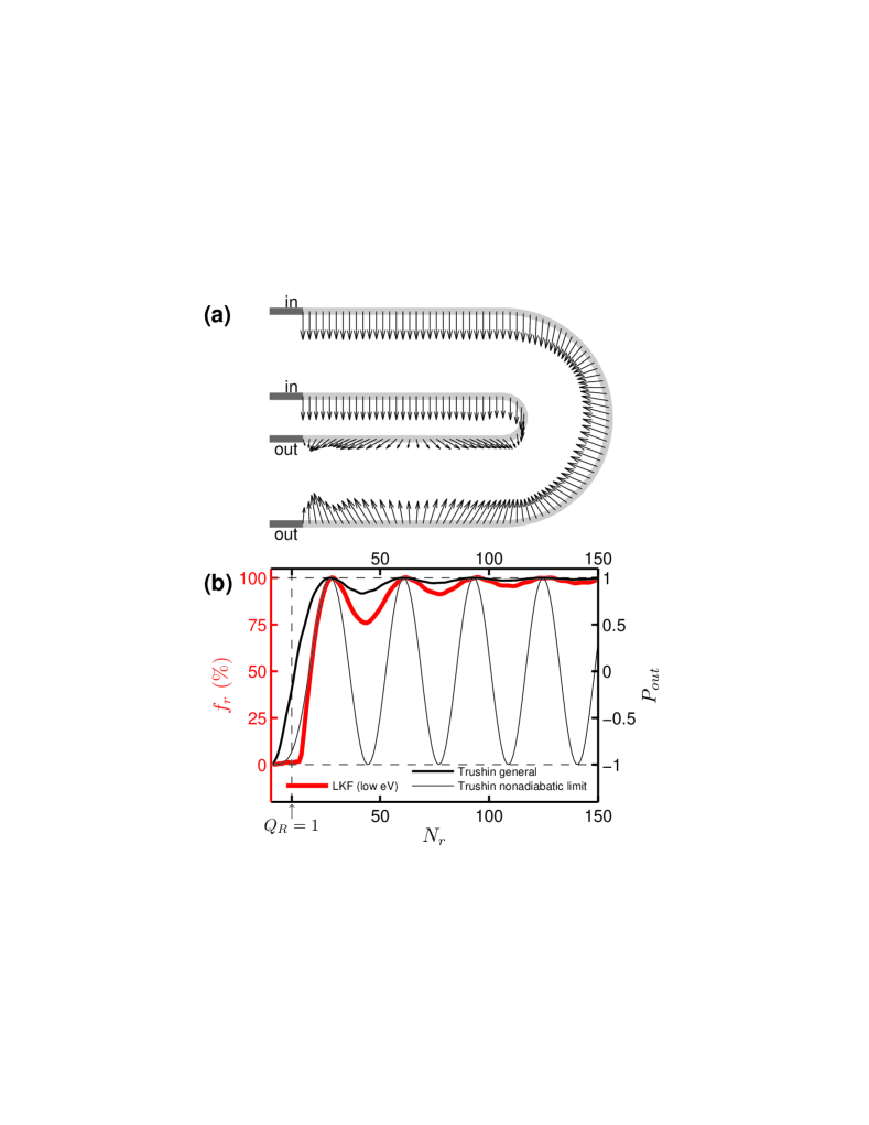
Figure 4: (Color online) (a) Top view of the spin density vectors shown in Figs. 2(a) and 3(a) with high bias. (b) Spin flip ratio $f_{r}$ as a function of $N_{r}$ with $(t_{R},t_{D})=(0.1,0)t_{0}$ and the output spin polarization based on Ref. Trushin and Chudnovskiy, 2006; the nonadiabatic curve is given by Eq. (47).

To make a quantitative investigation, we first define the following spin-flip ratio,

$$f_{r}\equiv\frac{1}{\pi}\cos^{-1}\left(\frac{\mathbf{S}_{L}\cdot\mathbf{S}_{R}}{\left|\mathbf{S}_{L}\right|\left|\mathbf{S}_{R}\right|}\right)\frac{\left|\mathbf{S}_{R}\right|}{\left|\mathbf{S}_{L}\right|}\times 100\%,$$ (44)

where $\mathbf{S}_{L}$ and $\mathbf{S}_{R}$ are the average spin direction of the left and right arms, respectively, computed by the LKF. In the case of the Rashba U-channel with $S^{x}$ injection, the spin is flipped from $+S^{x}$ to $-S^{x}$ when reaching the right arm, if the local eigenstate is strictly followed. Thus the definition of Eq. (44) helps us quantify how well the local eigenstate is followed: whether a change in direction or a shrink in the magnitude reduces the spin-flip ratio. Note that Eq. (44) is also valid for pure Dresselhaus U-channels, provided that the injected spin has to be oriented along $\pm y$, due to the $180{{}^{\circ}}$ turn of the U-channel. That is, as long as the spin transport is sufficiently adiabatic, the injected spin is able to follow the local eigenstate so that the spin is flipped after passing through the half-ring region.

Let us first fix the Rashba SOC strength as $t_{R}=0.1t_{0}$ but change the half-ring from small radius to larger ones, as shown in Fig. 4(b), where a clear jump at about $N_{r}=16$ is observed. Within $N_{r}\lesssim 16$ the spin-flip ratio is nearly zero, showing that the spin can hardly follow the local spin eigenstate when entering the half-ring region. At right side of the jump, $f_{r}$ increases to 100% and then exhibits a resonance-like oscillation below the maximum value, in close analogy to Ref. Trushin and Chudnovskiy, 2006 and similar to some of the results reported in Ref. Zhang et al., 2007. The oscillation period of about $32$ corresponds to a distance for the spin to complete a $2\pi$ of precession angle under the Rashba SOC, i.e., two times the spin precession length,Nikolić et al. (2005)

$$L_{so}/a=\frac{\pi}{2}\frac{t_{0}}{t_{R}}.$$ (45)

Here we have $2L_{so}/a=10\pi$. This oscillation period can be well described by Ref. Trushin and Chudnovskiy, 2006, which we will discuss later.

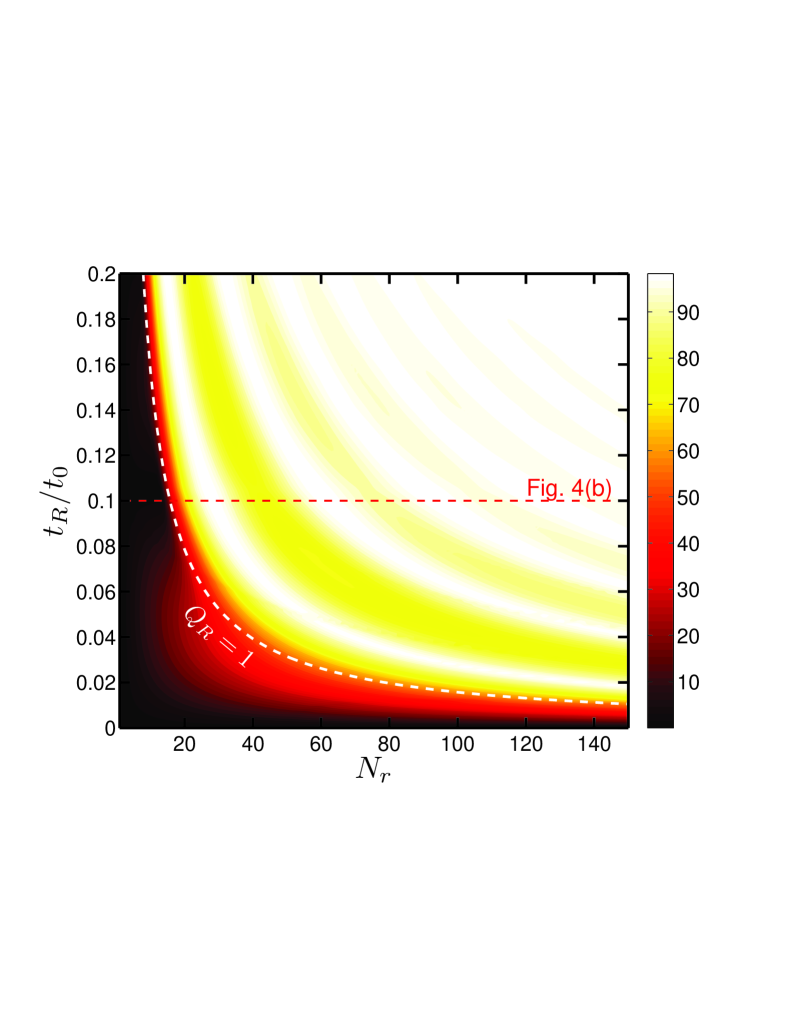
Figure 5: (Color online) Spin-flip ratio $f_{r}$ defined in Eq. (44) as a function of $t_{R}$ and $N_{r}$, free of $t_{D}$. The white dashed line given by $Q_{R}=1$ divides the transport into nonadiabatic (left-bottom) and adiabatic (right-top) regimes. Horizontal dashed line corresponds to Fig. 4(b).

The jump of $f_{r}$ and the wavelength of the resonance-like oscillation depends on the SOC strength. Hence we next vary both Rashba strength and the site number of the half-ring, and make the plot for $f_{r}$ as a function of $t_{R}$ and $N_{r}$ in Fig. 5. The $f_{r}$ pattern is clearly divided into two regimes that can be perfectly described by the $Q_{R}=1$ curve, which was inspired by Ref. Frustaglia and Richter, 2004. The adiabatic condition was previously argued asStern (1992); Aronov and Lyanda-Geller (1993) $Q\gg 1$, where $Q=Q_{B}+Q_{R}$ includes the contribution from external magnetic field and the Rashba field. In our analysis no external magnetic field is applied, and the adiabatic condition reads $Q_{R}\gg 1$. The definition of $Q_{R}$ from Ref. Frustaglia and Richter, 2004 is here reexpressed in terms of our tight-binding parameters,

$$Q_{R}=\frac{2}{\pi}\frac{t_{R}}{t_{0}}N_{r},$$ (46)

which implies that the increase of either $N_{r}$ or $t_{R}$ brings the transport regime to adiabatic. Therefore the criterion that $Q_{R}\gg 1$ preserves the transport in the adiabatic regime is well agreed. Furthermore, by a comparison with Eq. (45), the meaning of $Q_{R}$ given by Eq. (46) is transparent: $Q_{R}=N_{r}/\left(L_{so}/a\right),$ i.e., the number of precession half-periods that the spin can complete within the half-ring. Hence the condition $Q_{R}=1$ from our notation corresponds exactly to the arc length of the half-ring that matches one spin precession length $L_{so}$. The mathematical criterion for adiabatic transport, within which the electron spins are able to follow the local field, means that the electron spins have to be able to complete at least an angle of $\pi$ of precession within the half-ring. One might attempt to extend this interpretation to an arbitrary expanding angle of an arc, such as the curvilinear QW considered in Ref. Zhang et al., 2007, but further examination is left here as a possible extending work.

Finally, we compare our result with that of Ref. Trushin and Chudnovskiy, 2006, which is shortly reviewed in the following. Trushin and Chudnovskiy previously considered also a U-shaped 1D channel with Rashba SOC and solved the transmission problem by matching the boundary conditions.Trushin and Chudnovskiy (2006) A spin polarization was defined as $P=(j^{+}-j^{-})/(j^{+}+j^{-})$, where $j^{\pm}$ is the probability current of the $\pm$ eigenspin components. The polarized wave occupying the $+$ Rashba eigenstate was assumed as the incoming state so that $P_{in}=1$ and the spin polarization for the outgoing wave $P_{out}$ is the main quantity of interest. If the injected spin remains at its local eigenstate, $P_{out}=1$ is expected, which is the adiabatic limit. Oppositely, a strong nonadiabatic limit leads to a simplified expression,Trushin and Chudnovskiy (2006)

$$P_{out}=\cos\left(\pi Q_{R}\sqrt{1+Q_{R}^{-2}}\right),$$ (47)

which has been translated to our tight-binding language. As shown in Fig. 4(b), the oscillation matches our result; the curves in the low $N_{r}$ region ($Q_{R}$ small) match particularly well. For larger $Q_{R}$, Eq. (47) approaches $\cos(\pi Q_{R})$ with the oscillation period $\Delta Q_{R}=2=\Delta N_{r}/(L_{so}/a)$, which well describes the period of $\Delta N_{r}=2L_{so}/a$ in Fig. 4(b), in agreement with our previous discussion. For general $Q_{R}$, $P_{out}$ can be computed following their results and is plotted also in Fig. 4(b) (with $t_{R}=0.1t_{0}$ and $E_{F}=0.2t_{0}$). Overall, the oscillation behavior in both the nonadiabatic and general cases from Ref. Trushin and Chudnovskiy, 2006 agrees with our result.

In the above discussion, we have injected an $S^{x}$ spin, which is the eigenstate of the Rashba wire. The fact that the eigenstates in the ring differ from those in the wire by a tilt angle is the origin that a spin starting with $S^{x}$ in the U-channel can never perfectly follow the local eigenstate in the half-ring part. In principle, when the spin direction happens to match the ring eigenstate when the electron is just about to enter the ring, the local ring eigenstate can then be well followed. In the following section, we will show that these special cases do exist, provided that the length $L$ and the orientation angle of the injected spin are precisely designed.

III.3 More on charge and spin transport

The last goal to be carried out here is to reveal some of the interesting transport properties, regarding both charge and spin, based on quantum transport calculations.

III.3.1 Charge density modulation: Emergence of spin-orbit potential

As previously remarked in Sec. III.1.1 [or specifically the bottom panel of Fig. 2(b)], an additional modulation to the low-bias charge density in the half-ring region appears when both terms of SOCs are present. In Fig. 6(a), we show the formation of this charge density modulation in a $\left(N_{w},N_{r}\right)=\left(50,100\right)$ U-channel by fixing $t_{D}=0.02t_{0}$ and varying from $t_{R}=0$ to $t_{R}=t_{D}$, with $eV_{0}=10^{-3}t_{0}$ and $E_{F}=0.2t_{0}$. Clearly, the modulation appears only when $t_{R}t_{D}\neq 0$ and reaches its maximum when both SOCs are of the same strength. This modulation was similarly obtained in a recent study of the anisotropic spin transport in mesoscopic rings,Wang and Chang (2008) but the origin there was not clear. In the following we provide a simple quantum mechanical picture to account for this modulation.

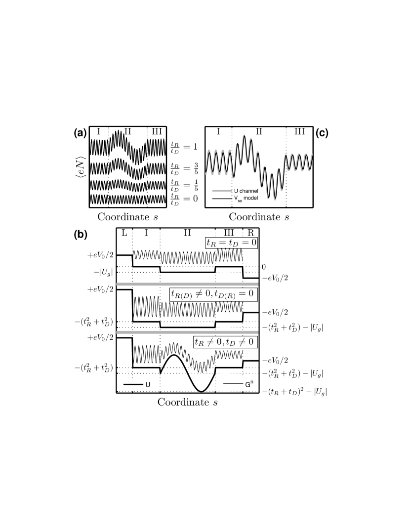
Figure 6: (a) Formation of the charge density modulation in a $\left(N_{w},N_{r}\right)=\left(50,100\right)$ U-channel with $eV_{0}=10^{-3}t_{0}$, $t_{D}$ fixed at $0.02t_{0}$, and $t_{R}$ varied from $0$ to $t_{D}$. (b) 1D Schrödinger problem for a 1D linear chain subject to the spin-orbit potential model. The top, middle, and bottom panels account for the zero SOC, single type of SOC, and mixed type of SOCs, respectively. Parameters used here are identical to the U-channel shown in (a). In addition to regions I, II, and III that correspond to those in the U-channel, the left (L) and right (R) leads are also labeled. (c) Local charge density $\langle eN\rangle$ for the U-channel and the electron correlation function $G^{n}\propto\left|\psi\left(s\right)\right|^{2}$ for the linear chain, both considering $t_{R}=t_{D}=0.02t_{0}$. Calculations here are all with $E_{F}=0.2t_{0}$.

Recall the anisotropic spin splitting, Eq. (29). By solving for $k_{\pm}$ from $E_{F}=\hbar^{2}k_{\pm}^{2}/2m\pm\zeta k_{\pm}$ and defining the Fermi wave vector as $k_{F}=\left(k_{+}+k_{-}\right)/2$, we have

$$k_{F}a=\sqrt{\frac{E_{F}}{t_{0}}+\left(\frac{t_{so}}{t_{0}}\right)^{2}},$$ (48)

where

$$t_{so}\left(\phi_{k}\right)=\frac{\zeta}{2a}=\sqrt{t_{R}^{2}+t_{D}^{2}-2t_{R}t_{D}\sin 2\phi_{k}}.$$ (49)

The fact that the Fermi wavelength $\lambda_{F}=2\pi/k_{F}$ is forced (when $t_{R}t_{D}\neq 0$) to be modulated upon changing propagation angle $\phi_{k}$ can be mapped to a linear 1D chain with a position-dependent local potential. Defining

$$\frac{V_{so}}{t_{0}}=-\left(\frac{t_{so}}{t_{0}}\right)^{2},$$ (50)

Eq. (48) then reads $k_{F}a=\sqrt{\left(E_{F}-V_{so}\right)/t_{0}}$, as if the electron were propagating in a 1D linear system subject to a potential $V_{so}$, i.e., the electron is governed by $\left(p^{2}/2m+V_{so}\right)\psi=E\psi$. This interpretation is exact when $V_{so}$ is a constant potential; when $V_{so}$ is position dependent but weak compared with $E_{F}$, the argument is still a good approximation.

We therefore consider a 1D linear chain subject to, together with the geometric potential, the full local potential,

$$U\left(s\right)=\begin{cases}V_{so}\left(+\pi/2\right),&s\in\left[0,L\right]\\ V_{so}\left(\phi_{k}\right)+U_{g},&s\in\left[L,L+\pi r\right]\\ V_{so}\left(-\pi/2\right),&s\in[L+\pi r,2L+\pi r]\end{cases},$$ (51)

where $\phi_{k}$ as a function of $s$ is taken identical to Eq. (30). The 1D Schrödinger problem subject to the potential $U(s)$ given by Eq. (51), $\left[-\hbar^{2}\partial^{2}/2m\partial s^{2}+U(s)\right]\psi(s)=E\psi(s)$, can be analytically cumbersome due to the irregular shape of $U(s)$, but can be easily solved by the quantum transport formalism introduced in Sec. II.2.1 at an even lower cost. The lead self-energy, Eq. (20), with $t_{M}=0$ is taken for both left and right leads (with potentials $+eV_{0}/2$ and $-eV_{0}/2$, respectively) to simulate the incoming and outgoing waves. The squared norm of the wave function in such an equilibrium problem corresponds to the electron correlation function $G^{n}\left(E\right)$ (equivalent to $-iG^{<}$) that can be obtained from $f_{0}\left(E\right)A\left(E\right)$.Datta (1995) The Fermi function $f_{0}$ will be taken as unity, concerning the currently assumed zero temperature, and the spectral function $A$ can be obtained from $A=G^{R}\Gamma G^{A}$, where $G^{R}$ and $G^{A}$ are the retarded and advanced Green’s function of the linear chain, respectively; the broadening function is given by $\Gamma=i(\Sigma_{L}-\Sigma_{L}^{{\dagger}})$. Note that we have turned off the contribution of the right lead to the broadening function to suppress the inflow of the particles from the right leads. This is equivalent to setting the wave function in the outgoing region as $\left.\psi\left(s\right)\right|_{s\geq L+\pi r}\propto e^{+iks}$, which is a usual assumption taken in most quantum physics textbooks.

The potential profile $U\left(s\right)$ together with $G^{n}\propto\left|\psi\left(s\right)\right|^{2}$ is plotted in Fig. 6(b) for three situations: zero SOC, single type of SOC, and mixed type of two SOCs. The last case clearly resembles the charge density modulation in the U-channel with $t_{R}t_{D}\neq 0$, and the present spin-orbit potential model seems to work well. Thus the modulation of the electron density profile simply reflects the position-dependent spin-orbit potential, Eq. (50), that is usually small compared with $E_{F}$. Indeed, in Fig. 6(c) we further compare the local charge density $\langle eN\rangle$ in the U-channel with the electron correlation function $G^{n}$ in the linear chain. The difference between them is only up to a tiny phase shift. Detailed parameters used here in Fig. 6 are given in the caption thereof.

When $\left|V_{so}\right|$ is close to $E_{F}$, either by strengthening the SOC parameters or lowering the Fermi energy, the phase shift grows, but the $G^{n}$ calculated for the linear chain and the $\langle eN\rangle$ calculated for the U-channel still are similar in their shapes (not shown). The present model hence works equally well to explain the charge density modulation, which we conclude as originating from the emergence of the angle-dependent spin-orbit potential when $t_{R}t_{D}\neq 0$.

III.3.2 Spin precession in special cases

In this subsection we discuss spin precessions in three special cases. In the first two cases, only one type of SOC is considered, and we inject the spin oriented as the theoretically predicted eigenstate for the ring (which is different from that for the wire), and adjust $t_{R}$ or $t_{D}$ such that the length $L$ equals exactly two times the spin precession length $L_{so}$. The injected spin arriving at the half-ring returns exactly to the eigenspin direction, such that the previously derived tilted eigenstate, e.g., the eigenspinor for clockwise-propagating $\downarrow$ eigenspinor in the Rashba ring from Ref. Frustaglia and Richter, 2004,

$$\chi_{R-}^{\downarrow}\left(\phi\right)=\left(\begin{array}[]{c}\sin\left(\gamma_{R}/2\right)\\ e^{i\phi}\cos\left(\gamma_{R}/2\right)\end{array}\right)=\left(\begin{array}[]{c}\cos[(\pi-\gamma_{R})/2]\\ e^{i\phi}\sin[(\pi-\gamma_{R})/2]\end{array}\right),$$ (52)

with the tilt angle $\gamma_{R}=\tan^{-1}Q_{R}$, can be numerically examined. Note that here $\phi$ is the azimuthal angle in the polar coordinate ($\phi=0$ defined along $+x$ axis), rather than the propagation angle $\phi_{k}$.

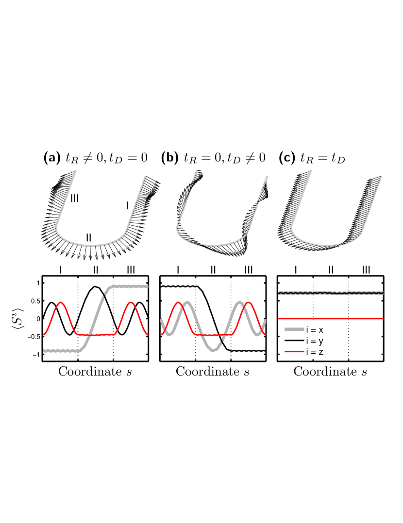
Figure 7: (Color online) Spin precession in a $\left(N_{w},N_{r}\right)=\left(50,50\right)$ U-channel with (a) $\left(t_{R},t_{D}\right)=\left(\pi/N_{w},0\right)t_{0}$, (b) $\left(t_{R},t_{D}\right)=\left(0,\pi/N_{w}\right)t_{0}$, and (c) $t_{R}=t_{D}=\left(\pi/\sqrt{2}N_{w}\right)t_{0}$. The injected spin is oriented in (a) as the Rashba ring eigenstate Eq. (52), in (b) as the Dresselhaus ring eigenstate Eq. (56), and in (c) as the persistent spin helix eigenstate Eq. (57). Note that in the imaging of the space-resolved spin vectors, only half of the vectors are drawn in order for clarity.

To account for the two extreme cases of pure Rashba and pure Dresselhaus using one single formula, we write the clockwise-propagating $\downarrow$ eigenspinor as

$$\chi_{-}^{\downarrow}\left(\phi\right)=\left(\begin{array}[]{c}\cos[(\pi-\gamma)/2]\\ e^{i\varphi}\sin[(\pi-\gamma)/2]\end{array}\right),$$ (53)

where $\varphi$ is given, similar to Eq. (27), as

$$\varphi=\arg\left[t_{R}\cos\phi-t_{D}\sin\phi+i\left(t_{R}\sin\phi-t_{D}\cos\phi\right)\right].$$ (54)

The tilt angle in Eq. (53) is given by

$$\gamma=\tan^{-1}\left(\sqrt{Q_{R}^{2}+Q_{D}^{2}}\right),$$ (55)

where $Q_{D}$ is defined similar to Eq. (46) as $Q_{D}=(2/\pi)(t_{D}/t_{0})N_{r}.$ Equation (53) clearly recovers the Rashba ring case of Eq. (52) since $\left.\varphi\right|_{t_{D}=0}=\phi$ from Eq. (54) and $\left.\gamma\right|_{t_{D}=0}=\gamma_{R}$ from Eq. (55), can cover the $t_{R}=0$ Dresselhaus ring case,

$$\chi_{D-}^{\downarrow}=\left(\begin{array}[]{c}\cos[(\pi-\gamma_{D})/2]\\ e^{-i(\pi/2+\phi)}\sin[(\pi-\gamma_{D})/2]\end{array}\right),$$ (56)

where $\gamma_{D}=\tan^{-1}Q_{D}$, but does not apply for general $t_{R}t_{D}\neq 0$ cases.

The last case is $t_{R}=t_{D}$, corresponding to the persistent spin-helix in 2DEG,Bernevig et al. (2006); Liu et al. (2006); Koralek et al. (2009) the main feature of which is the fixed eigenspin directions. In the present case, the $\downarrow$ eigenspinor is

$$\chi_{R=D}^{\downarrow}=\frac{1}{\sqrt{2}}\left(\begin{array}[]{c}e^{-i\pi/4}\\ 1\end{array}\right),$$ (57)

corresponding to $E_{k}=\hbar^{2}k^{2}/2m-\zeta k$. Whether this eigenstate, valid for 2DEG, still works in the curved 1D system, is what we are about to answer.

(a) Rashba ring eigenstate. We begin with $t_{D}=0$ and inject $\chi_{R-}^{\downarrow}\left(\phi=\pi\right)$ as given by Eq. (52) in a U-channel with $\left(N_{w},N_{r}\right)=\left(50,50\right)$. We tune $t_{R}/t_{0}=\pi/N_{w}\approx 0.063$ such that $N_{w}=\pi t_{0}/t_{R}=2L_{so}/a$ [see Eq. (45)] ensures the return of the injected spin to its initial spin direction, which is the eigenstate of the ring at $\phi=\pi$, after going through region I. As shown in Fig. 7(a), the spin entering the half-ring region remains perfectly in the eigenstate. (Note that we have chosen another view angle to focus on the half-ring part; injection conditions remain the same as in previous discussions.) The curves of $\langle S^{i}\rangle$ within region II can be well described by $\langle\chi_{R-}^{\downarrow}\left(\phi\right)|\vec{\sigma}|\chi_{R-}^{\downarrow}\left(\phi\right)\rangle$ [given below in Eq. (58)] with $\phi$ running from $\pi$ to $0$. The validity of the previously derived tilted eigenstate in Rashba rings is hence numerically verified.

Note the subtle difference between the special spin injection here and in Sec. III.2, where we injected an inplane $S^{x}$: an eigenstate of the wire. The precise design of the length $L$ and the orientation of the injected spin allows the spin to stay perfectly in the tilted ring-eigenstate. The $x$-component of spin with such a precise design can always be flipped, but should be regarded as a special situation.

(b) Dresselhaus ring eigenstate. We continue with $t_{R}=0$ and inject $\chi_{D-}^{\downarrow}\left(\phi=\pi\right)$ given by Eq. (56). In this case we similarly have $t_{D}/t_{0}=\pi/N_{w}$. Again the spin arriving at the half-ring enters its eigenstate and remains so until leaving the ring, as shown in Fig. 7(b). The spin components $\langle S^{i}\rangle$ within region II can be well described by $\langle\chi_{D-}^{\downarrow}\left(\phi\right)|\vec{\sigma}|\chi_{D-}^{\downarrow}\left(\phi\right)\rangle$, and the validity of the Dresselhaus ring eigenstate is also numerically verified. For both Figs. 7(a) and 7(b), spin components from Eq. (53),

$$\langle\chi_{-}^{\downarrow}\left(\phi\right)|\vec{\sigma}|\chi_{-}^{\downarrow}\left(\phi\right)\rangle=\left(\begin{array}[]{c}\sin\left(\pi-\gamma\right)\cos\varphi\\ \sin\left(\pi-\gamma\right)\sin\varphi\\ \cos\left(\pi-\gamma\right)\end{array}\right),$$ (58)

describes the $\langle S^{i}\rangle$ curves in region II well.

We remind the reader here that the eigenstate given by Eq. (53) is intended only for the two extreme cases of $t_{R(D)}\neq 0,t_{D(R)}=0$ discussed above, although a solution given in Ref. Wang and Vasilopoulos, 2005, similar to our Eq. (53), was claimed to be valid for rings in the presence of both Rashba and Dresselhaus terms. The simple reason why the form of Eq. (53) does not apply for general cases of $t_{R}t_{D}\neq 0$ is that the tilt angle $\gamma$ [Eq. (55)] does not recover $\pi/2$ when the $t_{R}=t_{D}\neq 0$ persistent spin helix state is reached, which is true as we will next numerically show.

(c) Persistent spin-helix eigenstate. We proceed by considering $t_{R}=t_{D}=(\pi/\sqrt{2}N_{w})t_{0}\approx 0.044t_{0}$, keeping the size of the U-channel unchanged. The injected spin state is oriented as $\chi_{R=D}^{\downarrow}$, given in Eq. (57). As expected, the injected spin stays at this eigenstate in region I, as shown in Fig. 7(c). Somewhat surprisingly, however, the injected spin remains precessionless throughout the whole U-channel, even in the half-ring region. Therefore, the persistent spin-helix eigenstate, originally derived for a 2DEG, is equally valid in straight wires and curved rings. This is in sharp contrast to the pure Rashba and pure Dresselhaus cases, for which the eigenstates in wires and in rings are different.

IV Experimental aspects

The U-shaped 1D channel theoretically discussed in the present paper can be experimentally prepared by using AFM lithography,Ihn (2010) i.e., local oxidationFuhrer et al. (2002) written by an AFM tip on the sample. The oxide lines turn out to completely deplete the 2DEG underneath, and can hence confine the electron gas in the desired nanostructure. A schematic sketch of the U-channel based on this technique is suggested in Fig. 1(c). According to the present fabrication ability (see, for example, Ref. Fuhrer et al., 2001), however, the ring radius is of the order of $100\unit{nm}$, and the induced geometric potential is rather weak: $10^{-2}$ $\mathop{\mathrm{m}eV}$ for GaAs-based quantum wells. To focus on the effect of the geometric potential, a single turn as in our U-channel is not enough; a series of geometric potential wells such as a sinelike waveguide similar to the design reported in a recent experiment on photonic crystalSzameit et al. (2010) may give rise to a resonance that could potentially be measured.

The spin injection assumed here may be realized either electrically or optically. The former requires a ferromagnetic source contact and may further complicate the sample fabrication and even the transport properties. The latter, optical spin injection, has been mature in generating spin packets that can be electrically manipulated.Flatté and Ţifrea (2007) Regarding the U-channel sketched in Fig. 1(c), the adiabatic-nonadiabatic spin transport discussed here may be experimentally tested by optically pumping at the source a spin packet that can be electrically dragged to the drain end by applying a bias voltage between the source and the drain contacts. Optical spin detection of the spin packet at the drain end shows whether the spin is reversed (adiabatic), is decayed (spin relaxed), or remains (nonadiabatic), compared with the injected spin direction. The laser spot size for the optical spin injection or detection, typically of a few hundreds of microns, may impose a corresponding limit on the design but could be possibly overcome by hard masks. A top gate covering the U-channel may control the Rashba SOC strengthNitta et al. (1997); Grundler (2000); Bergsten et al. (2006) and switch the transport regimes between adiabatic and nonadiabatic, provided that the effect of the Dresselhaus term is well treated.

Experimental proof of the interesting charge and spin transport properties discussed in Sec. III.3 are also expected. In particular, the charge density modulation in the presence of both Rashba and linear Dresselhaus (001) SOCs discussed in Sec. III.3.1 requires measurement on the local charge densities only and should be possible. The profile of the charge density modulation simply reflects the angle-dependent spin-orbit potential and hence determines the type of the SOCs: flat for the single type of SOC and sinelike for the mixed type of SOC. Note that in our discussion of the U-channel, the nature of $\sin 2\phi$ dependence of the spin-orbit potential provides the modulation in the half-ring with one period of the sine function. In the case of a full ring, we expect two periods then.

An alternative to preparing a 1D channel is the V-groove QW based on electron beam lithography,Ihn (2010) but so far application of this technique to curved 1D QWs has not been seen.

V Conclusion

In conclusion, we have rederived the Hamiltonian for a curved 1D structure in the presence of SOC. Applied to the 1D ring, the Hamiltonian is not only consistent with the previously proposed proper Hamiltonian for a Rashba ring,Meijer et al. (2002) but also contains a curvature-induced geometric potential, which was first derived in Ref. da Costa, 1981, but less discussed in the literature of ring issues. The U-shaped 1D channel is further taken to be a specific example to investigate the role of this geometric potential, as well as to compare the spin densities obtained by the LKF with the previous quantum mechanical approaches. Both translationLiu and Chang (2006) and spin-orbit gaugeChen and Chang (2008) methods mostly agree with the LKF results, even though the underlying assumption is rather simplified: to assume an ideally injected spin at the initial position, and the technique is rather artificial: to drag the injected spin by operating quantum operators. Whether the SVF,Liu and Chang (2006) a further approximating result from the translation method, may work well or not depends on whether the orthogonality approximation [Eq. (25)] is valid enough: exact for a straight 1D structure, of moderate error for a ring with a single type of SOC, and poor for a ring with a mixed type of SOCs.

The influence of the geometric potential taken into account in the LKF calculation is shown to be sensible only when the turn of the channel is sharp and the transport is under low bias. Overall the role played by the geometric potential is moderate, just like a local potential well, and can be drastic [such as the reversal of the injected spin state shown in Fig. 3(a) or 3(c)] only when a certain resonance condition is reached.

We have also discussed the spin transport in adiabatic and nonadiabatic regimes. In addition to the increase of the geometric potential when making the turn sharper by reducing the number of site $N_{r}$ in the turning part, the transport becomes nonadiabatic since the change of the local eigenstate becomes rapid. The spin transport shows adiabatic behavior when the turn is smooth and the SOC is strong enough, which agrees with the previously stated adiabatic condition.Stern (1992); Aronov and Lyanda-Geller (1993); Frustaglia and Richter (2004) We have also compared our results with a recent similar work by Trushin and Chudnovskiy,Trushin and Chudnovskiy (2006) which showed good agreement.

The last part of the numerical results revealed interesting charge and spin transport properties. For charge transport, the interplay between the Rashba and linear Dresselhaus (001) SOCs leads to anisotropic spin splitting, and hence an angle-dependent Fermi wavelength. Charge transport in a curved 1D chain subject to a modulated Fermi wavelength is therefore mapped to transport in a 1D linear chain subject to a position-dependent potential. We have shown that the charge density modulation that appears only when $t_{R}t_{D}\neq 0$ in the half-ring part of the U-channel can be well explained by the spin-orbit potential model. For spin transport, we have shown spin precession patterns in three special cases, which are equivalent to numerically testing the validity of the previously predicted tilted eigenstates of the Rashba rings and Dresselhaus rings, as well as that of the persistent spin-helix state.