TomograPy: A Fast, Instrument-Independent, Solar Tomography Software.

Abstract

Solar tomography has progressed rapidly in recent years thanks to the development of robust algorithms and the availability of more powerful computers. It can today provide crucial insights in solving issues related to the line-of-sight integration present in the data of solar imagers and coronagraphs. However, there remain challenges such as the increase of the available volume of data, the handling of the temporal evolution of the observed structures, and the heterogeneity of the data in multi-spacecraft studies. We present a generic software package that can perform fast tomographic inversions that scales linearly with the number of measurements, linearly with the length of the reconstruction cube (and not the number of voxels) and linearly with the number of cores and can use data from different sources and with a variety of physical models: TomograPy (http://nbarbey.github.com/TomograPy/), an open-source software freely available on the Python Package Index. For performance, TomograPy uses a parallelized-projection algorithm. It relies on the World Coordinate System standard to manage various data sources. A variety of inversion algorithms are provided to perform the tomographic-map estimation. A test suite is provided along with the code to ensure software quality. Since it makes use of the Siddon algorithm it is restricted to rectangular parallelepiped voxels but the spherical geometry of the corona can be handled through proper use of priors. We describe the main features of the code and show three practical examples of multi-spacecraft tomographic inversions using STEREO/EUVI and STEREO/COR1 data. Static and smoothly varying temporal evolution models are presented.

iint iiint

1 Introduction

sec:introduction

1.1 Motivation

Except for the rare case when in-situ exploration is practicable, the properties of astronomical objects are deduced from the analysis of the properties of light only. Most astrophysical measurements are therefore affected by the problem of line-of-sight (LOS) integration, i.e. the modification of the signal of interest by background and foreground emission and absorption. This problem is one of the major sources of uncertainties in the diagnostics of the solar plasma.

Integration along the LOS tends to confuse structures to the point that measurements crucial to the understanding of coronal physics are difficult to interpret. The controversy about the nature of polar plumes is one example. Polar plumes are observed at visible and UV wavelengths extending quasi-radially over the solar poles. Their appearance in photographic records led to the classical view of plumes as being pseudo-cylindrical structures denser than the surrounding corona. However such linear features in the images can also result from chance alignments of fainter structures distributed along a network pattern and integrated along the LOS. Both types of plumes have been supported by different authors, and it is possible that the two types coexist. See, e.g., gabriel2009 for a detailed discussion. Since the two proposed types of plumes have nearly identical properties in remote-sensing data, the true nature of these objects remains a subject of controversy.

One can also cite the problem of background estimation in the coronal-loop debate. As building blocks of the solar corona, loops have been extensively studied. However, we still cannot answer fundamental questions such as what processes are responsible for their formation or for their heating. One of the factors explaining this state of facts is that the determination of physical parameters such as density and temperature within the loops is rendered difficult by LOS superimposition. For example, terzo2010 have shown that different estimations of the loop-background radiation lead to different temperature profiles and different conclusions regarding the loop cooling.

Different strategies have been devised over the years to overcome the limitations imposed upon remote-sensing data by LOS integration. One obvious approach is to select an observation time when the solar corona presents a simple geometry for which it is possible to estimate the contribution of the various regions of the LOS. When observing polar plumes, for example, data are acquired preferentially at solar minimum when the polar holes are well developed so that the contribution of streamers to the foreground and background is minimum. However, even if these conditions are met, it is likely that several plumes or plumes and inter-plumes are superimposed along the LOS, thus confusing the interpretation. Therefore, favorable observing conditions are generally not sufficient to exclude possible LOS ambiguity.

If a simple coronal configuration cannot be assumed, or more generally if superimpositions cannot be ruled out, one has to devise means of analyzing the LOS content. Spectroscopic techniques such as the Differential Emission Measure (DEM) can be used to estimate the quantity of emitting plasma along the LOS as a function of temperature. If this approach is able to detect the presence of regions of different temperatures along the LOS, it does not say how the temperatures are distributed spatially. A single multithermal volume can have the same DEM signature as the superimposition of several large-scale isothermal structures.

Line-of-sight ambiguities can be alleviated, at least partially, if one can make several simultaneous observations from different locations. The twin spacecraft of the STEREO mission [Kaiser et al. (2008)] were designed to achieve this. The two vantage points that they offer provide precious information on the LOS content. In some cases, especially with a high-contrast object having well-defined boundaries such as coronal loops, direct stereoscopic reconstructions can be performed. Such reconstructions can, for example, be used to assess the quality of the background estimation used in loop studies (e.g. aschwanden2008). However for more diffuse objects not presenting sharp boundaries, or for which the visible boundaries can be LOS-integration artifacts, such as streamers, plumes, etc., direct, stereoscopic reconstruction is not reliable. However, if two viewpoints or more are available, tomography is a possible approach to inverting the LOS integration.

1.2 Solar Tomography

The term tomography encompasses a wide range of techniques aimed at imaging the internal structure of objects. Tomographic techniques are used in many areas of scientific research such as medicine, geophysics, materials science, and astrophysics. In the particular case of solar tomography, images recording the line-of-sight integration of coronal emission and taken from different viewpoints are used to estimate local physical quantities such as the electron number density or temperature. This is achieved using computed tomographic reconstruction techniques identical to the ones used in medical computer tomography. Mathematically, it is an inversion of the line-of-sight integration. This method is sometimes called Solar Rotational Tomography (SRT) as it generally relies upon the solar rotation to simulate data acquisition from different viewpoints.

However, there is significant differences between SRT and medical computer tomography that renders the problem more difficult to solve in the case of SRT. First, medical imaging scenarios benefit from high signal to noise ratio (SNR) measurements and have much higher measurement density than what is currently available with solar observatories. But more importantly, medical imaging has much less restriction on the number of point-of-view. Indeed, most of the time, SRT is restricted to one instantaneous point-of-view, the only exception being the STEREO twin spacecrafts. Another important difference with medical imaging is the presence of an opaque sphere in the middle of the region of interest: the photosphere. A similar issue is the presence of occulter in coronograph instruments, which restricts spatial information available in the data. This renders the problem much more ill-posed in SRT than in medical imaging tomography.

Progress in solar tomography comes from the availability of new data, new physical models, new inversion algorithms, and more powerful computers. Solar tomography can be traced back to van1950electron who presented a one-dimensional inversion of white-light data by fitting an analytic corona model.

Another seminal paper of SRT is altschuler1972determining. It introduced computer aided numerical estimation of the three-dimensional electron density of the corona using data from the K-coronameter of the High Altitude Observatory. The method reduces to a least-square estimation of the coefficients of Legendre polynomials.

Later, davila1994solar investigated, through simulations, the possibility of performing full three-dimensional (3D) solar tomography of the corona. That article assumed that more than one spacecraft would take data (up to nine actually) and thus did not require data to be taken at different times. Emission-map estimation was performed using the algebraic reconstruction technique (ART) which is an iterative gradient method used to invert the linear tomographic model. Estimated maps where reduced to $20\times 20$ grids.

With the availability of the Solar and Heliospheric Observatory (SOHO) data came the first three-dimensional maps of the corona both in white light (e.g. frazin2002tomography) with the Large Angle Spectrometric Coronagraph (LASCO: brueckner1995lasco) and in the ultraviolet (e.g. panasyuk1999three) using the UltraViolet Coronagraph Spectrometer (UVCS: kohl1995). An algorithm-oriented article by frazin2000tomography introduced a penalized likelihood approach minimized using an iterative solver (conjugate-gradient) to allow noise mitigation through proper regularization and modeling of the outliers.

Several generalizations were then developed. For example, wiegelmann2003magnetic introduced a method for the joint estimation of the electron density and the magnetic field while frazin2009 proposed a reconstruction of the local DEM from EUV images.

The temporal evolution of coronal structures during data acquisition is one of the main issues in coronal tomography. Two different directions have been investigated to address this issue: either assume slow evolution (e.g. butala2010dynamic) or further restricting the possible evolution to specific structures (e.g. barbey2008time).

1.3 Outline

In this article we describe TomograPy, an open-source software package implementing the main desirable features in a generic solar tomography code (see, e.g., frazin2005rotational for a review): capability to use both EUV and white-light data to estimate the local electron density and temperature, modeling the temporal evolution of structures during data acquisition, and performing rotational tomography with multiple spacecraft, i.e. with STEREO data.

In Section sec:tomographic_inversion we formulate mathematically the tomographic inversion problem and introduce the notations used in the description of the code given in Section sec:features. Section sec:performances gives an overview of the numerical performance of the code while Section sec:exemples describes three practical examples of tomographic reconstructions.

2 Tomographic Inversion

2.1 Linear Inverse Problem

sec:tomographic_inversion The problem to invert can be expressed by Equation (eq:linear) where ${\mathb{y}}$ is the data, ${\mathb{A}}$ is called the physical model, ${\mathb{x}}$ is the object map to estimate, and ${\mathb{n}}$ is an additive noise (which we will assume Gaussian, independent and identically-distributed (iid))

$${\mathb{y}}={\mathb{A}}{\mathb{x}}+{\mathb{n}}\ilabel{eq:linear}$$ (1)

The physical model represents all of the transformations that link the quantity to estimate (e.g. the local emissivity, electron temperature, electron density, etc.) to the data. It always includes the line-of-sight integration and the model of temporal evolution, even if this later is implicitly static. The physical model may also include the formation process of the observed lines if one wants to estimate a physical quantity such as the local electron density or temperature instead of the local emissivity. We restrict ourselves to cases where the data are a linear function of the unknown quantities to determine. It is worth noting, however, that tomographic inversion can be done even if the physical model is non-linear, although accompanied by an important increase in complexity. An exemple of non-linear tomography application is electrical capacitance tomography soleimani2005nonlinear which is intrinsically non linear. Using Monte Carlo Markov Chain (MCMC) methods, it would be feasible to fit non-linear models of Coronal Mass Ejections as the one provided in thernisien2009forward.

2.2 Bayesian View on Linear Inversion

In the Bayesian paradigm, a probability density function (PDF) is associated with each variable. To invert the class of problems described by Equation (eq:linear), one needs to know the statistical properties of the noise [${\mathb{n}}$], which gives the likelihood. One also needs to define a prior on the unknowns [${\mathb{x}}$]: it gives the PDF of ${\mathb{x}}$ knowing the data [${\mathb{y}}$], which is called the posterior on ${\mathb{x}}$. This is done through Bayes’ rule given in Equation (eq:bayes)

$$f({\mathb{x}}|{\mathb{y}},\mathcal{M})=\frac{f({\mathb{y}}|{\mathb{x}},\mathcal{M})f({\mathb{x}}|\mathcal{M})}{f({\mathb{y}}|\mathcal{M})}\ilabel{eq:bayes}$$ (2)

where $\mathcal{M}$ regroups all of the assumptions on the model. In this article, the PDF of ${\mathb{x}}$ given ${\mathb{y}}$ is noted $f({\mathb{x}}|{\mathb{y}})$.

In the case of a Gaussian multivariate likelihood and prior, the posterior is also Gaussian, and thus fully determined by its mean and covariance matrix. This is summed up in Equation (eq:gaussian_bayes)

eq:gaussian_bayes$$f({\mathb{x}}|\mathcal{M}) \sim \mathcal{N}({\mathbf{0}},\sigma_{\mathb{x}}^{2}({\mathb{B}}^{T}{\mathb{B}})^{-1})$$

$$f({\mathb{y}}|{\mathb{x}},\mathcal{M}) \sim \mathcal{N}({\mathb{A}}{\mathb{x}},\sigma_{\mathb{n}}^{2}{\mathb{I}})$$

$$f({\mathb{x}}|{\mathb{y}},\mathcal{M}) \sim \mathcal{N}(\hat{{\mathb{x}}},\hat{{\boldsymbol{\Sigma}}})$$

$$\hat{{\mathb{x}}} = \hat{{\boldsymbol{\Sigma}}}{\mathb{A}}^{T}{\mathb{y}}$$ (3)

$$\hat{{\boldsymbol{\Sigma}}} = \left({\mathb{A}}^{T}{\mathb{A}}+\lambda{\mathb{B}}^{T}{\mathb{B}}\right)^{-1}$$

$$\lambda = \frac{\sigma_{\mathb{x}}^{2}}{\sigma_{\mathb{n}}^{2}}$$

where $\mathcal{N}({\boldsymbol{\mu}},{\boldsymbol{\Sigma}})$ is a multivariate Gaussian of mean ${\boldsymbol{\mu}}$ and covariance ${\boldsymbol{\Sigma}}$. In Equation (eq:gaussian_bayes) we assumed an independent Gaussian noise of variance $\sigma_{n}^{2}$, so that the covariance of the likelihood is $\sigma_{n}^{2}{\mathb{I}}$ where ${\mathb{I}}$ is the identity matrix. We defined a zero-mean prior [$f({\mathb{x}}|\mathcal{M})$] with ${\mathb{B}}$ being a prior model. ${\mathb{B}}$ can be, for instance, a finite-difference operator. A zero-mean prior combined with a finite-difference operator means that the finite difference of the map tends to be close to zero. In other words, this prior would favor smoother solutions over non-smooth solutions close to the data. This is a sensible choice for electron density at the scales considered. $\sigma_{n}$ and consequently $\lambda$ are free parameters. It is possible to assign a PDF to $\lambda$ in order to estimate this parameter in an unsupervised way but it results generally in very resource-consuming algorithms. In this article, we will restrict ourselves to a fixed $\lambda$ in a supervised way.

Characterizing the solution in a Bayesian way requires the estimation of both $\hat{{\boldsymbol{\Sigma}}}$ and $\hat{{\mathb{x}}}$. $\hat{{\mathb{x}}}$ gives the most probable solution and $\hat{{\boldsymbol{\Sigma}}}$ gives information about the uncertainties in the unknowns. However, in most practical cases, the covariance matrix [$\hat{{\boldsymbol{\Sigma}}}$] is too large to be stored in memory, and one only keeps $\hat{{\mathb{x}}}$. In this case, a full matrix inversion is not required, and one can estimate ${\mathb{x}}$ much faster using iterative schemes such as the conjugate gradient method.

Since ${\mathb{x}}$ is the maximum a posteriori (MAP) of the problem, it is also the minimum of the co-log–likelihood as written in Equation (eq:criterion)

eq:criterion$$\hat{{\mathb{x}}} = \displaystyle\mathop{\mathrm{arg\,min}}_{{\mathb{x}}}\left\{{J({\mathb{x}})}\right\}$$

$$= \displaystyle\mathop{\mathrm{arg\,min}}_{{\mathb{x}}}\left\{{-\log\left[f({\mathb{x}}|{\mathb{y}},\mathcal{M})\right]}\right\}$$

$$= \displaystyle\mathop{\mathrm{arg\,min}}_{{\mathb{x}}}\left\{{-\log\left[f({\mathb{y}}|{\mathb{x}},\mathcal{M})f({\mathb{x}}|\mathcal{(}M))\right]}\right\}$$

$$= \displaystyle\mathop{\mathrm{arg\,min}}_{{\mathb{x}}}\left\{{\left\|{\mathb{y}}-{\mathb{A}}{\mathb{x}}\right\|^{2}+\lambda\left\|{\mathb{B}}{\mathb{x}}\right\|^{2}}\right\}$$

$$= \left({\mathb{A}}^{T}{\mathb{A}}+\lambda{\mathb{B}}^{T}{\mathb{B}}\right)^{-1}{\mathb{A}}^{T}{\mathb{y}}$$

The term $\|{\mathb{y}}-{\mathb{A}}{\mathb{x}}\|^{2}$ is a simple least-squares term. It defines the closeness to the data. The second term [$\|{\mathb{B}}{\mathb{x}}\|$] is a regularization term that prevents the estimate from being noisy. In terms of matrix inversion, ${\mathb{A}}^{T}{\mathb{A}}$ is ill-conditioned and ${\mathb{B}}^{T}{\mathb{B}}$ is added in order to have a better-conditioned matrix. To find $\hat{{\mathb{x}}}$, iterative-gradient methods need only the definition of the criterion $J({\mathb{x}})$ and its gradient $\nabla_{\mathb{x}}J$. Gradient methods can be order of magnitudes faster than the full inversion of the matrix, especially when A and B are sparse or when the problem has been properly preconditioned.

3 Main Features of TomograPy

sec:features

3.1 Fast Parallelized Projector

subsec:projector TomograPy is a Python [Van Rossum and Centrum voor Wiskunde en Informatica (1995)] package build around a C implementation of the Siddon algorithm [Siddon (1985)] of line-of-sight integration, and is thus restricted to rectangular parallelepiped voxels. This C projector has been parallelized using OpenMP [Dagum and Menon (2002)]. Numpy [Oliphant (2006)] is a requirement as well as PyFITS [Barrett and Bridgman (1999)] to handle FITS data files. Optionally, one can use SciPy [Jones, Oliphant, and Peterson (2001–)] sparse matrix optimization routines to perform fast linear inversions. The algorithm has been carefully optimized using meta-programming techniques to avoid if statements and function pointers in the inner loop. This has been done using templates of C code, and replacing key values in the source template to generate variations in the C sources for various application (e.g.: float and double values, projection and backprojection, presence of an obstacle or not). Here the word template is not to be confused with C++ templates but is more closy related to the notion of web template. The same idea is used in Numpy itself and allow more flexibility to pure C code.

The projection algorithm provided with TomograPy can be used with a variety of estimation methods as long as they rely on the linear-operator interface. It allows for fast testing of various optimization strategies. Results presented in this article will exclusively use conjugate gradient schemes, but TomograPy provides other options. The key requirement is for the algorithm to rely on matrix–vector operations.

See Section sec:performances for an analysis of the performance and scaling of this implementation. The TomograPy projector is well tested and provided with a test suite, which fully covers this part of the code.

3.2 Instrument Independence

TomograPy takes as input FITS files (Flexible Image Transport System: wells81) containing fully calibrated images expressed in units consistent with the physical model chosen by the user. TomograPy internally uses the World Coordinate System (WCS) [Calabretta and Greisen (2002), Greisen and Calabretta (2002)] standard keywords to determine the position of the observer and to define the projector from the data and the desired format of the object map. TomograPy will therefore accept any data compliant with the WCS standard. As the data of most current instruments are already provided as WCS-compliant FITS files, all that is required is to store a set of calibrated files in a directory that TomograPy will be pointed to. For data that does not conform to WCS, it is straightforward to write a small wrapper that will handle the instrument-specific metadata and convert them into the corresponding WCS keywords.

TomograPy allows inversions using data from multiple spacecraft, for example with STEREO-A and B and SOHO. The data from the different instruments nonetheless need to be consistent, i.e. to record the same physical quantity.

3.3 Physical models

As stated in section sec:tomographic_inversion, any linear model can be inverted using the same framework. TomograPy provides with the possibility to perform inversions with the several models described in this section. The TomograPy projector already discussed in Section subsec:projector is a building block for all of the models described here. We will first describe models of temporal evolution and then models of line emission. It is possible to combine these models to perform, for example, multi-spacecraft, smooth, temporal rotational tomography. In the future, it will be possible to combine the models presented here with models not yet available in TomograPy such as the Differential Emission Measure model [Frazin, Vásquez, and Kamalabadi (2009)] or magnetic-field models [Wiegelmann and Inhester (2003)].

3.3.1 Single Spacecraft Static Tomography

subsec:substatic This is the simplest case. In the next two sections we will consider only the line-of-sight inversion without assumptions on the line formation process. In this case, static rotational tomography of the solar corona can easily be formulated as in Equation (eq:linear) once discretized. In this article, we will assume that the object-map cube has been discretized using contiguous rectangular parallelepiped voxels of identical shape; it is a requirement of the Siddon algorithm. Since the intensity on one detector results from the integration along the line of sight of the emission in the observed object, it can be expressed as in Equation (eq:lo):

$$y_{j}=\sum_{i}P_{i,j}e_{i}+n_{j}\ilabel{eq:lo}$$ (5)

where $y_{j}$ is the intensity of the detector $j$, $e_{i}$ is the emission in the voxel $j$, and $P_{i,j}$ is the length of the segment of the line of sight $i$ that corresponds to the voxel $j$, and $n_{j}$ is the noise observed on detector $j$. Reformulating Equation (eq:lo) in terms of vectors and matrices, we obtain Equation (eq:lo_t) where the $t$ index refers to the time at which the data have been taken.

$${\mathb{y}}_{t}={\mathb{P}}_{t}{\mathb{e}}_{t}+{\mathb{n}}_{t}\ilabel{eq:lo_{t}}$$ (6)

where ${\mathb{P}}$, the TomograPy projector, is the most basic block for building physical models. Note that we indexed both axes of the detector using one index as well as the voxels of the object map. We can do the same on a time index, since we assume that there is no temporal evolution (${\mathb{e}}$ does not vary with $t$). Regrouping all of the data at all considered instants [$t$], results in Equation (eq:srt) which is similar to Equation (eq:linear).

$${\mathb{y}}=\left(\begin{array}[]{c}{\mathb{y}}_{1}\\ \vdots\\ {\mathb{y}}_{T}\end{array}\right)=\left(\begin{array}[]{c}{\mathb{P}}_{1}\\ \vdots\\ {\mathb{P}}_{T}\end{array}\right){\mathb{e}}+\left(\begin{array}[]{c}{\mathb{n}}_{1}\\ \vdots\\ {\mathb{n}}_{T}\end{array}\right)={\mathb{P}}{\mathb{e}}+{\mathb{n}}\ilabel{eq:srt}$$ (7)

This model can be used to estimate emission maps from EUV data using formula (eq:criterion). We can use a smoothness prior to avoid having too much noise in the maps. This is done using a finite-difference operator along each axis of the maps for the ${\mathb{B}}$ matrix. If we want to account for the lower signal-to-noise ratio that we typically have in solar rotational tomography, we can have finite-difference operators weighted by the altitude of the considered voxels. Finally, we have the following equation

$$\ilabel{eq:srt_{i}nversion}\hat{{\mathb{e}}}_{SRT}=\displaystyle\mathop{\mathrm{arg\,min}}_{{\mathb{e}}}\left\{{\left\|{\mathb{y}}-{\mathb{P}}{\mathb{e}}\right\|^{2}+\lambda\left\|{\mathb{D}}{\mathb{R}}{\mathb{e}}\right\|^{2}}\right\}$$ (8)

where ${\mathb{D}}$ is the finite-difference operator and ${\mathb{R}}$ is a diagonal operator with the height of the voxels on the diagonal. The use of a smoothness prior increasing linearly with height, allows for the maps not to be affected by the difference between spherical grids and Cartesian grids. Spherical grids have bigger voxels at high altitudes increasing the SNR per voxel with height. This is not the case for Cartesian grids but it is compensated by the use of a height-dependent prior.

3.3.2 Multiple-Spacecraft Static Tomography

subsec:multistatic If now we want to use data from multiple spacecraft, with the static assumption we can use Equation (eq:two_spacecraft) (assuming two spacecraft A and B without loss of generality).

$${\mathb{y}}_{A} = g_{A}{\mathb{P}}_{A}{\mathb{e}}+{\mathb{n}}_{A}$$

$${\mathb{y}}_{B} = g_{B}{\mathb{P}}_{B}{\mathb{e}}+{\mathb{n}}_{B}$$ (9)

Each of Equations (eq:two_spacecraft) are derived from (eq:srt) but both spacecraft can have different gains ($g_{A}$ and $g_{B}$) at the wavelength considered. In this model, it is not possible to assume a different behavior of the filters as a function of the wavelength since ${\mathb{e}}$ needs to correspond to emission integrated in one filter. Fortunately, this assumption is valid to a good approximation for several existing instruments. The passbands of the two Extreme UltraViolet Imagers (EUVI: wuelser2004euvi) on STEREO and those of the Extreme ultraviolet Imaging Telescope (EIT: delaboudiniere1995eit) have for example been designed to be identical.

Equation (eq:two_spacecraft) can be reformulated as Equation (eq:linear) by a simple concatenation as shown in Equation (eq:lin2space).

$${\mathb{y}}_{A,B}=\left(\begin{array}[]{c}{\mathb{y}}_{A}\\ {\mathb{y}}_{B}\end{array}\right)=\left(\begin{array}[]{c}g_{A}{\mathb{P}}_{A}\\ g_{b}{\mathb{P}}_{B}\end{array}\right){\mathb{e}}+\left(\begin{array}[]{c}{\mathb{n}}_{A}\\ {\mathb{n}}_{B}\end{array}\right)={\mathb{P}}_{A,B}{\mathb{e}}+{\mathb{n}}_{A,B}\ilabel{eq:lin2space}$$ (10)

Finally, multiple-spacecraft tomography in the static case can be formulated as single-spacecraft tomography as long as all of the instruments have the same spectral bandwidth. The only modification is the multiplication by gains, which vary from one instrument to the other. We can then write the estimated map using Equation (eq:criterion) as in Equation (eq:srt_multiple_inv).

$$\ilabel{eq:srt_{m}ultiple_{i}nv}\hat{{\mathb{e}}}_{SRT,A,B}=\displaystyle\mathop{\mathrm{arg\,min}}_{{\mathb{e}}}\left\{{\left\|{\mathb{y}}_{A,B}-{\mathb{P}}_{A,B}{\mathb{e}}\right\|^{2}+\lambda\left\|{\mathb{D}}{\mathb{R}}{\mathb{e}}\right\|^{2}}\right\}$$ (11)

Using a DEM model, it is possible to extend multiple-spacecraft tomography to cases in which the spacecraft have different bandpasses since the spectral response is then integrated into the model. This is the approach followed by [Frazin, Vásquez, and Kamalabadi (2009)].

3.3.3 Smooth temporal tomography

subsec:smooth Because the corona is not static, dynamic models are desirable. In this case however, it is no longer possible to simplify Equation (eq:lo_t) as in Equation (eq:srt). When temporal evolution is present, the recording of data taken at different times can be expressed as

$${\mathb{y}}=\left(\begin{array}[]{c}{\mathb{y}}_{1}\\ \vdots\\ {\mathb{y}}_{T}\end{array}\right)=\left(\begin{array}[]{ccc}{\mathb{P}}_{1}&&{\mathbf{0}}\\ &\ddots&\\ {\mathbf{0}}&&{\mathb{P}}_{T}\end{array}\right)\left(\begin{array}[]{c}{\mathb{e}}_{1}\\ \vdots\\ {\mathb{e}}_{T}\end{array}\right)+\left(\begin{array}[]{c}{\mathb{n}}_{1}\\ \vdots\\ {\mathb{n}}_{T}\end{array}\right)={\mathb{P}}_{\mathcal{T}}{\mathb{e}}_{\mathcal{T}}+{\mathb{n}}\ilabel{eq:srt_{t}}$$ (12)

This results in a highly underdetermined inverse problem since there are $T$ times more unknowns than in Equation (eq:srt). This underdetermination can be mitigated using either priors, such as a temporal smoothness prior, or a parameterization of the temporal evolution. Thus a classic, smooth, temporal solar-rotational tomography (STSRT) would perform conjugate gradient estimation using the criterion given in Equation (eq:stsrt), where ${\mathb{D}}_{r}$ and ${\mathb{D}}_{t}$ are the finite-difference operators in space and time. Typically, due to strong underdetermination, the hyperparameter $\lambda_{t}$ would be greater than $\lambda_{r}$, favoring solutions with small temporal changes.

$$\hat{{\mathb{e}}}_{STSRT}=\left\|{\mathb{y}}-{\mathb{P}}_{\mathcal{T}}{\mathb{e}}_{\mathcal{T}}\right\|^{2}+\lambda_{r}\left\|{\mathb{D}}_{r}{\mathb{e}}_{\mathcal{T}}\right\|^{2}+\lambda_{t}\left\|{\mathb{D}}_{t}{\mathb{e}}_{\mathcal{T}}\right\|^{2}\ilabel{eq:stsrt}$$ (13)

This kind of approach using spatio-temporal regularization has been explored before [Zhang, Ghodrati, and Brooks (2005), Khalsa and Fessler (2007)].

Following the same approach as in Section subsec:multistatic, it is possible to generalize this expression to the case of multiple spacecraft.

3.4 EUV Lines

In the case of EUV lines or EUV bands, the dominant formation process of the observed radiation is excitation by collisions between ions and electrons. The local emissivity can thus be supposed to be isotropic in which case the quantity inverted in Sections subsec:substatic to subsec:smooth is directly the local emissivity of the plasma summed over the spectral response of the instrument. Resonant scattering may contribute significantly to EUV bands such as the 17.1 nm and 19.5 nm bands used in, e.g., TRACE, EIT, EUVI, and AIA [Schrijver and McMullen (2000)]. If this is confirmed, then the local emissivity is not isotropic and one needs to apply a correction factor to the inverted quantities to deduce plasma emissivities.

3.5 White Light: Thomson Scattering

In the case of white-light detectors, the measured intensity is largely dominated by Thomson scattering of the photospheric radiation by free coronal electrons. Figure fig:thomson_corona shows the geometry of Thomson scattering in the corona. Following billings66, the equations of Thomson scattering in the corona are

Figure 1.: Geometry of Thomson scattering in the corona. $M$ is the location of the scattering electron, $O$ is Sun center, $S$ is an emission point on the solar surface, $D$ is the observer, and $T$ is the tangent to the solar surface. $\rho$ is the impact parameter of $(DM)$, $r$ is the distance of the scattering point to Sun center, $R_{\odot}$ is the solar radius. $\Omega$ is the angle between the line of sight and the tangent to the solar surface passing through the scattering point.fig:thomson_corona

$$\begin{array}[]{rcl}I_{t}&=&\frac{\pi\sigma}{2}\frac{I_{0}}{r^{2}}n_{e}\left[(1-u)C_{3}+uC_{4}\right]\\ I_{t}-I_{r}&=&\frac{\pi\sigma}{2}\frac{I_{0}}{r^{2}}n_{e}\frac{\rho^{2}}{r^{2}}\left[(1-u)C_{1}+uC_{2}\right]\\ \end{array}\ilabel{eq:thomson_{c}orona}$$ (14)

$$\begin{array}[]{rcl}C_{1}&=&\cos\Omega\sin^{2}\Omega\\ C_{2}&=&-\frac{1}{8}\left[1-3\sin^{2}\Omega-\frac{\cos^{2}\Omega}{\sin\Omega}(1+3\sin^{2}\Omega)\ln\left(\frac{1+\sin\Omega}{\cos\Omega}\right)\right]\\ C_{3}&=&\frac{4}{3}-\cos\Omega-\frac{\cos^{3}\Omega}{3}\\ C_{4}&=&-\frac{1}{8}\left[5+\sin^{2}\Omega-\frac{\cos^{2}\Omega}{\sin\Omega}(5-\sin^{2}\Omega)\ln\left(\frac{1+\sin\Omega}{\cos\Omega}\right)\right]\end{array}\ilabel{eq:4C}$$ (15)

where $u$ accounts for the center-to-limb variation and is a function of wavelength, $I_{t}$ and $I_{r}$ are intensities in the radial and transverse directions, $n_{e}$ is the electron density, $r$ is the distance of the scattering point to the center of the Sun, $\rho$ is the impact parameter of the line of sight, $\Omega$ is the angle between the line of sight and the tangent to the solar surface passing through the scattering point, $\sigma$ is the Thomson-scattering cross-section and $I_{0}$ is the incident intensity.

The important point in these equations is that the intensity is a linear function of the electron density. It is thus possible to directly estimate the electron density using solar tomography on white-light data. Note also that the Thomson-scattering equations can be separated into coefficients that depend on the position [$M$] in the corona (through $r$ and $\Omega$) and the line of sight (through the impact parameter [$\rho$]). These coefficients are given in Equation (eq:thomson_lo).

$$\begin{array}[]{ccc}o_{k}&=&\rho^{2}_{k}\\ m_{j}&=&\frac{(1-u)C_{1}(r_{j})+C_{2}(r_{j})}{r_{j}^{4}}\\ m^{\prime}_{j}&=&\frac{(1-u)C_{3}(r_{j})+C_{4}(r_{j})}{r_{j}^{2}}\\ \end{array}\ilabel{eq:thomson_{l}o}$$ (16)

Measurements are generally decomposed into a polarized brightness [pB] component and a total brightness [B] component. Equation (eq:brightness) gives the equations for those quantities.

$$pB_{k} = \frac{\pi\sigma}{2}I_{0}\frac{\rho_{k}^{2}}{r_{j}^{4}}\left[(1-u)C_{1}(r_{j})+uC_{2}(r_{j})\right]n_{e,j}$$

$$B_{k} = \frac{\pi\sigma}{2}I_{0}\left\{-\frac{\rho_{k}^{2}}{r_{j}^{4}}\left[(1-u)C_{1}(r_{j})+uC_{2}(r_{j})\right]\right.$$ (17)

$$\left.+2\frac{1}{r_{j}^{2}}\left[(1-u)C_{3}(r_{j})+uC_{4}(r_{j})\right]\right\}n_{e,j}$$

From Equations (eq:thomson_lo) and (eq:brightness) one can build linear direct models for pB and B images as in Equation (eq:thomson_direct), where ${\mathb{n}}_{e}$ is the discretized electron-density map and ${\mathb{i}}_{pB}$ and ${\mathb{i}}_{B}$ are the pB and B images respectively. ${\mathb{O}}$, ${\mathb{M}}$, and ${\mathb{M}}^{\prime}$ are diagonal matrices with $o_{k}$, $m_{j}$, and $m^{\prime}_{j}$ on their diagonals.

$${\mathb{i}}_{pB} = {\mathb{T}}_{pB}{\mathb{n}}_{e}+{\mathb{n}}$$

$$= {\mathb{O}}{\mathb{P}}{\mathb{M}}{\mathb{n}}_{e}+{\mathb{n}}$$

$${\mathb{i}}_{B} = {\mathb{T}}_{B}{\mathb{n}}_{e}+{\mathb{n}}$$ (23)

$$= \left(\begin{array}[]{cc}-{\mathb{O}}&{\mathb{I}}\end{array}\right)\left(\begin{array}[]{cc}{\mathb{P}}&{\mathbf{0}}\\ {\mathbf{0}}&{\mathb{P}}\end{array}\right)\left(\begin{array}[]{c}{\mathb{M}}\\ {\mathb{M}}^{\prime}\end{array}\right){\mathb{n}}_{e}+{\mathb{n}}$$

Note that almost twice as much computation is required for simulation or inversion of total brightness data than for polarized brightness data. A recent application of this model can be found in frazin2010three.

4 Performance

sec:performances

We performed tests on a set of 64 images of 256 $\times$ 256 pixels, and a reconstruction cube of 128 $\times$ 128 $\times$ 128 voxels. We always use these parameters unless specified otherwise. For these tests there is no obstacle, meaning that the ray tracing is not interrupted as it would have been with the use of a model with an opaque photosphere. There is no mask applied to the data or the map. Tests have been done on a PC with two Quad-Core AMD Opteron^TM Processor 2380 and 32 Gigabytes of RAM.

In a more realistic use of TomograPy for solar tomography, the projections would be faster than presented here since masked pixels are not projected and LOS integration is stopped when the ray reaches the photosphere, reducing the number of computations.

Performance as a function of the number of threads used by OpenMP are shown in Table tab:ncores. It shows that the time to compute a projection and a back-projection is not exactly linear with the number of threads. It takes seven times less time to compute a projection with eight threads than with one thread and 6.1 times less to compute a back-projection. Back-projection does not scale as well as projection (the speed-up with multiple cores is better with the projection). This is due to the fact that extra care must be taken while updating the map of voxel values as opposed to the detector values in order to avoid race conditions. Race conditions are situation in which the outcome of a computation varies unexpectedly due to the timing of events in different threads. In TomograPy, race conditions occur mainly when two LOS need to update the same voxel at the same time. In the case of the projection, voxel values are only read, so this not an issue. Race conditions are avoided with the OpenMP atomic pragma directive which instruct each thread to update voxels sequentially, resulting in a slow-down of computations, but only for this part of the algorithm. Note however that the projections and back-projections scale better when the ratio between the number of data samples and the number of voxels decreases. Indeed, in this case, the number of lines of sight intersecting a single voxel decreases so that it is less probable that several threads try to update the same voxel at the same time.

Cores	1	2	3	4	5	6	7	8
Projection time [s]	97.5	48.6	36.3	26.4	21.2	18.2	16.8	13.9
back-projection time [s]	145.3	76.8	56.5	41.0	37.0	32.7	30.1	23.9

Table 1.: Performances of the projector as a function of threads.tab:ncores

Performance as a function of the image format is shown in Table tab:image_shape. As expected, the projection and back-projection duration scales linearly with the image size.

Image size	128 $\times$ 128	256 $\times$ 256	512 $\times$ 512	1024 $\times$ 1024
Projection time [s]	0.95	3.64	14.53	58.75
back-projection time [s]	1.61	6.17	24.69	99.54

Table 2.: Performance of the projector as a function of image shape.tab:image_shape

Performance as a function of the reconstruction cube size is shown in Table tab:cube_shape. We can see that the projection and back-projection duration scales linearly with the cube root of the number of voxels. This is expected as the number of voxels along a single LOS is roughly proportional to the number of voxels along one axis of the map and the number of operations is proportional with the number of intersections between LOS and voxels.

Cube size	1283	2563	5123	10243
Projection time [s]	13.84	44.56	195.69	587.56
back-projection time [s]	24.71	56.64	214.55	610.75

Table 3.: Performance of the projector as a function of the size of the reconstruction cube.tab:cube_shape

5 Examples

sec:exemples

5.1 Static Reconstruction using STEREO/EUVI A and B

We performed a conjugate gradient inversion using data from both EUVI A and B. To avoid issues due to differences in filters, we rescaled the EUVI B data to EUVI A levels by dividing by the empirically deduced values provided in Table tab:cross_cal_ab

bandwidth	171	195	284	304
B/A ratio	0.90	0.97	0.95	1.05

Table 4.: Ratio of sensitivity between EUVI A and EUVI B as a function of wavelength.tab:cross_cal_ab

This operation is justified since the passbands of the twin instruments were designed and were measured to be nearly identical. To first order, the difference in spectral response between EUVI A and B is a scaling factor. The image pairs where chosen to be simultaneous with a small lossy-compression factor. Because of the photosphere opacity, we need a full rotation (four weeks) to have data isotropic coverage of all parts of the reconstruction cube. If we focus only on the poles, this is no longer an issue and we can use only two weeks of data. We can also use the diversity of points of view provided by STEREO to reduce this duration. At the time of observation, the STEREO spacecraft were separated by 86^∘, reducing the acquisition time needed for a complete coverage of the corona to three weeks instead of a full solar rotation. For polar regions, the required acquisition time is further reduced to 11 days. We chose pairs of images regularly spaced from 1 to 15 December 2008, with four pairs of images per day and per observatory, resulting in 118 images. The estimated 3D map is a cube of $256\times 256\times 256$ voxels centered on the Sun with a width of three solar radii along each axis. In order to save computation time while remaining consistent with the resolution of the reconstruction cube, the images were binned $2\times 2$. The Carrington rotation rate is assumed.

Figure (fig:srt) shows the local emissivity in the reconstructed cube at a constant altitude of 1.05 solar radii. An equi-rectangular projection is used.

Figure 2.: Reconstruction of the 17.1 nm local emissivity at 1.05 solar radii using STEREO/EUVI A and B data and assuming a static corona. Input data are 59 pairs of images equally spaced in time from 1 to 15 December 2008. The STEREO separation angle was 86^∘.fig:srt

As can be seen, part of the projection around 300^∘ of longitude is smoother than the remainder of the projection. This is due to the fact that we used two weeks of data instead of the three weeks required to sample all voxels isotropically with lines of sight. To obtain a better estimate at these locations would have required the use of one more week’s data, which would have in turned worsened artifacts due to temporal evolution. Conversely, the polar regions are slightly oversampled because, considering the separation of the STEREO spacecraft, the minimum integration time was 11 days. Figure fig:srt_gnomo shows a gnomonic projection of the north polar region at 1.05 solar radii. The coronal hole is clearly visible as the darker central area. Structures in the hole are arranged according to a network pattern. One can identify bright nodules that could be attributed to the classical beam plumes but also elongated structures that could correspond to curtain plumes. This would confirm the proposition by gabriel2009 that both types of plumes coexist.

As can be seen, some of the voxels have negative values. This is usually explained as resulting from temporal evolution. Indeed, if temporal evolution has occurred during the acquisition of the data, it cannot be correctly modeled with the static assumption made in this inversion. Negative values are thus required to account for a variation of intensity in the data unexplainable by a simple change of viewpoint. This could also be explained by mismodeling of the measurement process, noise or even bias in the data (which could be due to some instrumental artifcat).

To show that convergence has indeed been reached with the conjugate gradient algorithm we present the criterion as a function of iteration number in Figure fig:criterion_exemple.

Figure 3.: Example of convergence criterion as a function of the iteration index.fig:criterion_exemple

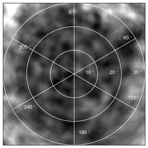
Figure 4.: Gonomic projection of the north pole at 1.05 solar radii. The reconstruction cube is the same as that of Figure fig:srt. This image can be compared with the dynamic reconstructions of Figure fig:stsrt.fig:srt_gnomo

5.2 Smooth Temporal Evolution with STEREO/EUVI A and B

The second example is a 3D map estimation using the smooth temporal evolution model. In other words, we minimize Equation (eq:stsrt) using the hyper-parameters stated in Table tab:hypers. We used the same set of EUVI images used for the static estimation. For each pair of EUVI images there is a corresponding instantaneous map of dimensions $128\times 128\times 128$, resulting in the estimation of approximately 132 millions of parameters. The estimation took less than eight hours.

Figure fig:stsrt shows gnomonic projections at 1.05 solar radii of the estimated map at different instants separated by 40 hours. It is interesting to compare these images with the static reconstruction of the same area shown in Figure fig:srt_gnomo. Here, the disappearance of an elongated structure at the south edge of the coronal hole is very clear, and one can also follow the appearance and disappearance of beam plumes.

model	$\lambda_{x}$	$\lambda_{y}$	$\lambda_{z}$	$\lambda_{t}$
SRT	$1e^{-1}$	$1e^{-1}$	$1e^{-1}$
Thomson	$1e^{-1}$	$1e^{-1}$	$1e^{-1}$
STSRT	$1e^{-1}$	$1e^{-1}$	$1e^{-1}$	$1e^{2}$

Table 5.: Hyper-parameters used for the inversion of the different models.tab:hypers

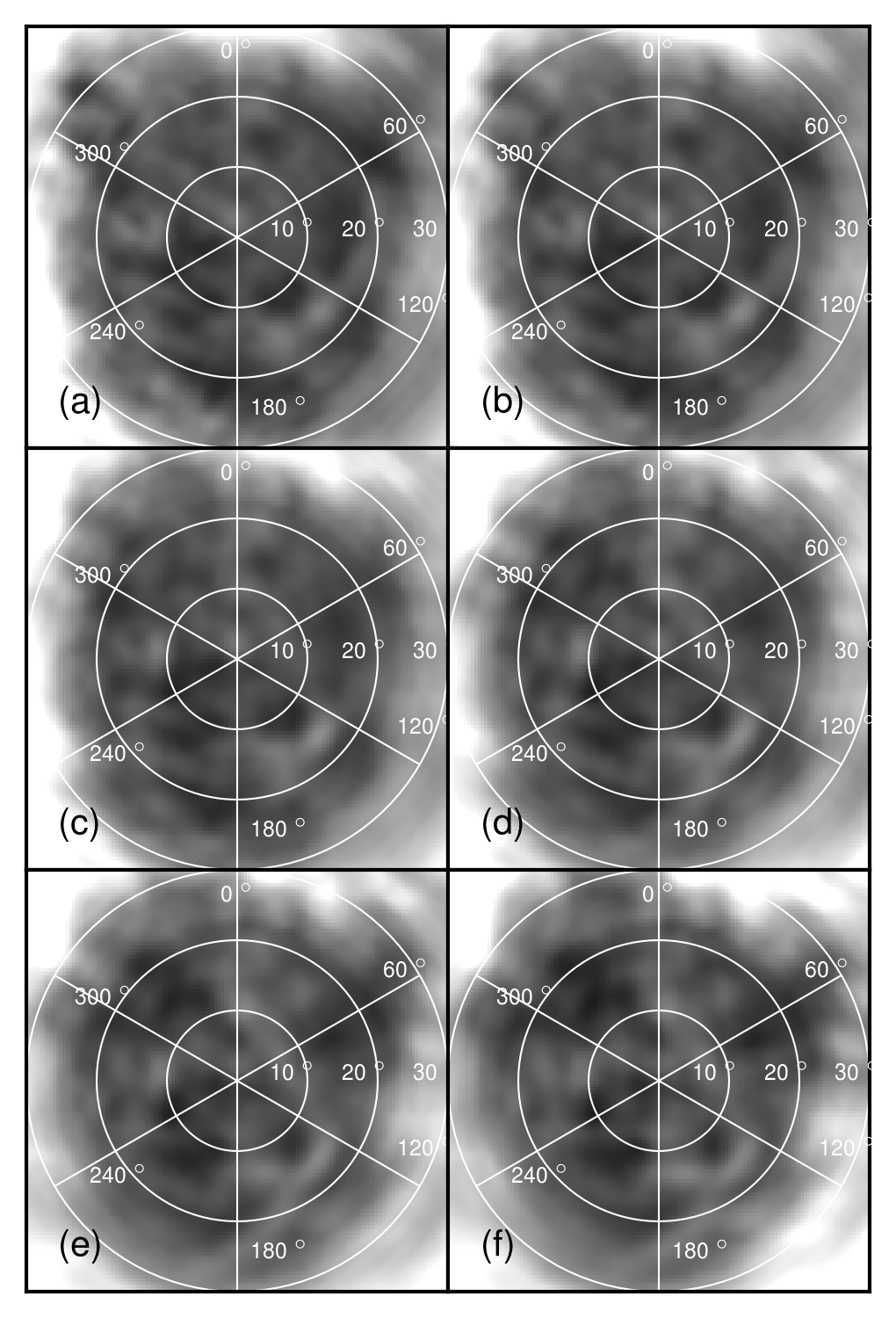
Figure 5.: Polar view of the emissivity at 1.05 solar radii from a temporally evolving 3D map estimation using STEREO/EUVI A and B data in the 17.1 nm passband. North pole gnomonic projection with a resolution of 1^∘ in square is used. There is 40 hours between each projection. These images can be compared with the static reconstruction of Figure fig:srt_gnomo.fig:stsrt

The static reconstruction is sharper than the temporally evolving one. This could be due to slower convergence in the smooth temporal-rotational tomography model. Indeed, since the temporal prior is much higher than the spatial prior, numerous very small steps in the conjugate-gradient algorithm could be required to reach the minimum. This could be missed by our stopping criterion on the norm of the gradient and even on convergence diagonstic such as the one in Figure fig:criterion_exemple. This could be solved through the use of preconditioning but has not been tried for now. However, one can clearly identify the sames structures in both reconstructions. One can picture the static reconstruction as a kind of average over time, although this is not strictly true as temporal effects and changes of viewpoints can have the same kind of effects on data.

5.3 Thomson scattering with COR1 A and B data

We estimated the coronal electron density using COR1 A and B data acquired during February 2008 as done by kramar2009tomographic. Since the inversion codes are different, the comparison gives an estimate of the robustness of both techniques. Our results are shown in Figure fig:thomson_inv and can be compared to Figure 2 of kramar2009tomographic. The comparison shows that very large scale structures are very similar in both maps, but fainter and smaller scales structures differ. This can be explained by the use of different prior models and hyper-parameters. Data can also differ in the way that they are prepared before the tomographic inversion. Note that we used a smoothness prior increasing with height for this reconstruction.

Figure 6.: Equi-rectangular projection of a static 3D map estimation using pB COR1 A and B data during February 2008 at 1.6 $R_{\odot}$ (a), 2.0 $R_{\odot}$ (b), and 2.4 $R_{\odot}$ (c). Pixels of the projections are 1^∘ square. fig:thomson_inv

6 Conclusions

sec:conclusions

We developed a tested, fast, and flexible program to perform rotational tomography of the solar corona. Its respect of WCS standards allows its use with virtually any data set available.

We demonstrated how this software can be used to perform multi-spacecraft estimations of emission maps in the corona using STEREO/EUVI data and STEREO/COR1 data. Estimations were performed using static, temporally-evolving, and Thomson-scattering models.

This new software suite can naturally be used to perform tomographic inversion of the corona using SDO/AIA images. TomograPy will allow tomographic estimation using AIA data at full resolution, providing unprecedented resolution as well as additional spectral information. Supplemented with spectral-inversion methods, this will allow for electron-density and temperature estimates in large data sets, close to the photosphere, at very high resolution.

Because of its modular architecture, TomograPy also provides a convenient way to test different estimation algorithms saving the need to rewrite anything other than the algorithm. This allows easy comparison of the performances of different algorithms for the solar tomography application.

References

- Altschuler and Perry (1972) Altschuler, M.D., Perry, R.M.: 1972, On determining the electron density distribution of the solar corona from K-coronameter data. Sol. Phys. 23(2), 410 – 428.
- Aschwanden et al. (2008) Aschwanden, M.J., Nitta, N.V., Wuelser, J.-P., Lemen, J.R.: 2008, First 3D Reconstructions of Coronal Loops with the STEREO A+B Spacecraft. II. Electron Density and Temperature Measurements. ApJ 680(2), 1477.
- Barbey et al. (2008) Barbey, N., Auchère, F., Rodet, T., Vial, J.C.: 2008, A Time-Evolving 3D Method Dedicated to the Reconstruction of Solar Plumes and Results Using Extreme Ultraviolet Data. Sol. Phys. 248(2), 409.
- Barrett and Bridgman (1999) Barrett, P., Bridgman, W.: 1999, PyFITS, a FITS module for Python. In: D. M. Mehringer, R. L. Plante, & D. A. Roberts (ed.) Astronomical Data Analysis Software and Systems VIII, Astronomical Society of the Pacific Conference Series 172, 483.
- Billings (1966) Billings, D.E.: 1966, A guide to the solar corona, Academic Press, New York.
- Brueckner et al. (1995) Brueckner, G.E., Howard, R.A., Koomen, M.J., Korendyke, C.M., Michels, D.J., Moses, J.D., Socker, D.G., Dere, K.P., Lamy, P.L., Llebaria, A., Bout, M.V., Schwenn, R., Simnett, G.M., Bedford, D.K., Eyles, C.J.: 1995, The Large Angle Spectroscopic Coronagraph (LASCO). Sol. Phys. 162, 357.
- Butala et al. (2010) Butala, M., Hewett, R., Frazin, R., Kamalabadi, F.: 2010, Dynamic Three-Dimensional Tomography of the Solar Corona. Sol. Phys. 262(2), 495.
- Calabretta and Greisen (2002) Calabretta, M.R., Greisen, E.W.: 2002, Representations of celestial coordinates in FITS. A&A 395, 1077.
- Dagum and Menon (2002) Dagum, L., Menon, R.: 2002, OpenMP: an industry standard API for shared-memory programming. Comput. Science Eng., IEEE 5(1), 46.
- Davila (1994) Davila, J.M.: 1994, Solar tomography. ApJ 423, 871.
- Delaboudinière et al. (1995) Delaboudinière, J.P., Artzner, G., Brunaud, J., Gabriel, A.H., Hochedez, J.F., Millier, F., Song, X.Y., Au, B., Dere, K.P., Howard, R.A., et al.: 1995, EIT: extreme-ultraviolet imaging telescope for the SOHO mission. Sol. Phys. 162(1), 291.
- Frazin, Vásquez, and Kamalabadi (2009) Frazin, R.A., Vásquez, A.M., Kamalabadi, F.: 2009, Quantitative, Three-dimensional Analysis of the Global Corona with Multi-spacecraft Differential Emission Measure Tomography. ApJ 701, 547.
- Frazin (2000) Frazin, R.A.: 2000, Tomography of the solar corona. I. A robust, regularized, positive estimation method. ApJ 530, 1026.
- Frazin and Janzen (2002) Frazin, R.A., Janzen, P.: 2002, Tomography of the solar corona. II. Robust, regularized, positive estimation of the three-dimensional electron density distribution from LASCO-C2 polarized white-light images. ApJ 570, 408.
- Frazin and Kamalabadi (2005) Frazin, R.A., Kamalabadi, F.: 2005, Rotational tomography for 3D reconstruction of the white-light and EUV corona in the post-SOHO era. Sol. Phys. 228(1), 219.
- Frazin et al. (2010) Frazin, R.A., Lamy, P., Llebaria, A., Vásquez, A.M.: 2010, Three-Dimensional Electron Density from Tomographic Analysis of LASCO-C2 Images of the K-Corona Total Brightness. Solar Physics, 1 – 12.
- Gabriel et al. (2009) Gabriel, A.H., Bely-Dubau, F., Tison, E., Wilhelm, K.: 2009, The structure and origin of solar plumes: network plumes. ApJ 700, 551.
- Greisen and Calabretta (2002) Greisen, E.W., Calabretta, M.R.: 2002, Representations of world coordinates in FITS. A&A 395, 1061.
- Jones, Oliphant, and Peterson (2001–) Jones, E., Oliphant, T., Peterson, P.: 2001–, SciPy: Open source scientific tools for Python. http://www.scipy.org/.
- Kaiser et al. (2008) Kaiser, M., Kucera, T., Davila, J., St. Cyr, O., Guhathakurta, M., Christian, E.: 2008, The STEREO mission: An introduction. Space Sci. Rev. 136(1), 5.
- Khalsa and Fessler (2007) Khalsa, K.A., Fessler, J.A.: 2007, Resolution properties in regularized dynamic MRI reconstruction. In: Biomedical Imaging: From Nano to Macro, 2007. ISBI 2007. 4th IEEE International Symposium on, 456 – 459. IEEE. ISBN 1424406722.
- Kohl et al. (1995) Kohl, J.L., Esser, R., Gardner, L.D., Habbal, S., Daigneau, P.S., Dennis, E.F., Nystrom, G.U., Panasyuk, A., Raymond, J.C., Smith, P.L., Strachan, L., van Ballegooijen, A.A., Noci, G., Fineschi, S., Romoli, M., Ciaravella, A., Modigliani, A., Huber, M.C.E., Antonucci, E., Benna, C., Giordano, S., Tondello, G., Nicolosi, P., Naletto, G., Pernechele, C., Spadaro, D., Poletto, G., Livi, S., von der Lühe, O., Geiss, J., Timothy, J.G., Gloeckler, G., Allegra, A., Basile, G., Brusa, R., Wood, B., Siegmund, O.H.W., Fowler, W., Fisher, R., Jhabvala, M.: 1995, The Ultraviolet Coronagraph Spectrometer for the Solar and Heliospheric Observatory. Sol. Phys. 162, 313.
- Kramar et al. (2009) Kramar, M., Jones, S., Davila, J., Inhester, B., Mierla, M.: 2009, On the Tomographic Reconstruction of the 3D Electron Density for the Solar Corona from STEREO COR1 Data. Sol. Phys. 259(1), 109.
- Oliphant (2006) Oliphant, T.E.: 2006, A Guide to NumPy 1, Trelgol Publishing, USA.
- Panasyuk (1999) Panasyuk, A.V.: 1999, Three-dimensional reconstruction of UV emissivities in the solar corona using Ultraviolet Coronagraph Spectrometer data from the Whole Sun Month. J. Geophys. Res. 104(A5), 9721.
- Schrijver and McMullen (2000) Schrijver, C.J., McMullen, R.A.: 2000, A Case for Resonant Scattering in the Quiet Solar Corona in Extreme-Ultraviolet Lines with High Oscillator Strengths. ApJ 531, 1121.
- Siddon (1985) Siddon, R.L.: 1985, Fast calculation of the exact radiological path for a three-dimensional CT array. Medical Phys. 12, 252 – 255.
- Soleimani and Lionheart (2005) Soleimani, M., Lionheart, W.R.B.: 2005, Nonlinear image reconstruction for electrical capacitance tomography using experimental data. Measurement Science and Technology 16, 1987.
- Terzo and Reale (2010) Terzo, S., Reale, F.: 2010, On the importance of background subtraction in the analysis of coronal loops observed with TRACE. A&A 515, A7.
- Thernisien, Vourlidas, and Howard (2009) Thernisien, A., Vourlidas, A., Howard, R.: 2009, Forward modeling of coronal mass ejections using STEREO/SECCHI data. Solar Physics 256(1), 111 – 130.
- Van de Hulst (1950) Van de Hulst, H.: 1950, The electron density of the solar corona. Bull. Astronom. Inst. Netherlands 11, 135.
- Van Rossum and Centrum voor Wiskunde en Informatica (1995) Van Rossum, G., Centrum voor Wiskunde en Informatica: 1995, Python reference manual, Centrum voor Wiskunde en Informatica, Amsterdam.
- Wells, Greisen, and Harten (1981) Wells, D.C., Greisen, E.W., Harten, R.H.: 1981, FITS - a Flexible Image Transport System. Astron. and Astrophys. Supp. Ser. 44, 363.
- Wiegelmann and Inhester (2003) Wiegelmann, T., Inhester, B.: 2003, Magnetic modeling and tomography: First steps towards a consistent reconstruction of the solar corona. Sol. Phys. 214(2), 287.
- Wuelser et al. (2004) Wuelser, J.P., Lemen, J.R., Tarbell, T.D., Wolfson, C., Cannon, J.C., Carpenter, B.A., Duncan, D.W., Gradwohl, G.S., Meyer, S.B., Moore, A.S., et al.: 2004, EUVI: the STEREO-SECCHI extreme ultraviolet imager. In: Proceedings of SPIE 5171, 111.
- Zhang, Ghodrati, and Brooks (2005) Zhang, Y., Ghodrati, A., Brooks, D.H.: 2005, An analytical comparison of three spatio-temporal regularization methods for dynamic linear inverse problems in a common statistical framework. Inverse Problems 21, 357.