Evidence of a spin liquid phase in the frustrated honeycomb lattice

Abstract

In the present paper we present some new data supporting the existence of a spin-disordered phase in the Heisenberg model on the honeycomb lattice with antiferromagnetic interactions up to third neighbors along the line $J_{2}=J_{3}$, predicted in nos . We use the Schwinger boson technique followed by a mean field decoupling and exact diagonalization for small systems to show the existence of an intermediate phase with a spin gap and short range Néel correlations in the strong quantum limit $(S=\frac{1}{2})$.

I Introduction

Geometrical frustration in two-dimensional (2D) antiferromagnets is expected to enhance the effect of quantum spin fluctuations and hence suppress magnetic order giving rise to a spin liquid Anderson and this idea has motivated many researchers to look for its realization Sachdev1 ; Sachdev2 ; Sandvik ; Moessner ; Poilblanc .

One candidate to test these ideas is the honeycomb lattice, which is bipartite and has a classical Néel ground state, but due to the small coordination number $(z=3)$, quantum fluctuations could be expected to be stronger than those in the square lattice and may destroy the antiferromagnetic long-range order (LRO) Mattsson ; more .

The study of frustrated quantum magnets on the honeycomb lattice has also experimental motivations ESR ; libro_experimental ; exp_hex2 ; expnew1 ; expnew2 .

The analysis of the hexagonal lattice from a more general point of view has gained lately a lot of interest both coming from graphene-related issues and from the possible spin-liquid phase found in the Hubbard model in such geometry HubbardNature ; recent ; newer .

Motivated by the previous results, in this paper we show the study of the Heisenberg model on the honeycomb lattice with first ($J_{1}$), second ($J_{2}$) and third ($J_{3}$) neighbors couplings Fouet , along the special line $J_{2}=J_{3}$. Using Schwinger boson mean field theory (SBMFT) and exact diagonalization we find strong evidence for the existence of an intermediate disordered region where a spin gap opens and spin-spin correlations decay exponentially. Using exact diagonalization of small clusters we also have calculated the dimer-dimer correlation function that indicates short range dimer-dimer order. Although our results correspond to a specific line, we conjecture that the quantum disordered phase that we have found in the vicinity of the tricritical point extends within a finite region around it. Previous evidence of massive behaviour in the hexagonal lattice Heisenberg model has been found in other regions of the phase space by means of exact diagonalization in ref. Fouet .

The Heisenberg model on the $J_{1}-J_{2}-J_{3}$ honeycomb lattice is given by

$$H=J_{1}\sum_{\langle\mathbf{x}\mathbf{y}\rangle_{1}}\hat{\bf{S}}_{\mathbf{x}}\cdot\hat{\bf{S}}_{\mathbf{y}}+J_{2}\sum_{\langle\mathbf{x}\mathbf{y}\rangle_{2}}\hat{\bf{S}}_{\mathbf{x}}\cdot\hat{\bf{S}}_{\mathbf{y}}+J_{3}\sum_{\langle\mathbf{x}\mathbf{y}\rangle_{3}}\hat{\bf{S}}_{\mathbf{x}}\cdot\hat{\bf{S}}_{\mathbf{y}},$$ (1)

where $\hat{\bf{S}}_{\mathbf{x}}$ is the spin operator on site $\mathbf{x}$ and $\langle\mathbf{x}\mathbf{y}\rangle_{n}$ indicates sum over the $n$-th neighbors (see Fig. 1).

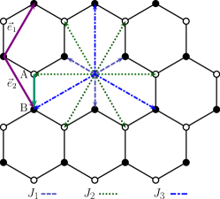
Figure 1: (Color online) Honeycomb lattice with sublattices A and B. The vectors $\vec{e}_{1}=(\frac{\sqrt{3}}{2},\frac{3}{2})$ and $\vec{e}_{2}=(\frac{\sqrt{3}}{2},-\frac{3}{2})$ are the primitive traslation vectors of the direct lattice.

In the classical limit, $S\to\infty$, the model displays different zero temperature phases with a tricritical point at $J_{2}=J_{3}=\frac{1}{2}J_{1}$. At this particular point the classical ground state has a large GS degeneracy Rastelli ; Fouet . The Heisenberg model on the honeycomb lattice was studied using SBMFT by Mattsson et al Mattsson for antiferromagnetic interactions at first and second neighbors. Here we study the Hamiltonian (1) using a rotationally invariant version of this technique, which has proven successful in incorporating quantum fluctuations Trumper1 ; Trumper2 ; Coleman .

II Schwinger bosons mean-field theory.

In this section we describe in detail the Schwinger boson mean field theory used in the present work. The $SU(2)$ Heisenberg Hamiltonian on a general lattice can be written as

$$\hat{H}=\frac{1}{2}\sum_{\mathbf{x}\mathbf{y}\alpha\beta}J_{\alpha\beta}(\mathbf{x}-\mathbf{y})\hat{\mathbf{S}}_{\mathbf{x}+\mathbf{r}_{\alpha}}\cdot\hat{\mathbf{S}}_{\mathbf{y}+\mathbf{r}_{\beta}},$$ (2)

where $\mathbf{x}$ and $\mathbf{y}$ are the positions of the unit cells and vectors $\mathbf{r}_{\alpha}$ correspond to the positions of each atom within the unit cell. $J_{\alpha\beta}(\mathbf{x}-\mathbf{y})$ is the exchange interaction between the spins located in $\mathbf{x}+\mathbf{r}_{\alpha}$ e $\mathbf{y}+\mathbf{r}_{\beta}$.

In what follows we assume that the classical order can be parameterized as

$$\hat{S}^{x}_{\mathbf{x}+\mathbf{r}_{\alpha}} = S\sin\varphi_{\alpha}(\mathbf{x})$$ (3)

$$\hat{S}^{y}_{\mathbf{x}+\mathbf{r}_{\alpha}} = 0$$ (4)

$$\hat{S}^{z}_{\mathbf{x}+\mathbf{r}_{\alpha}} = S\cos\varphi_{\alpha}(\mathbf{x}),$$ (5)

with $\varphi_{\alpha}(\mathbf{x})={\bf Q}\cdot\mathbf{x}+\theta_{\alpha}$, where ${\bf Q}$ is the ordering vector and $\theta_{\alpha}$ are the relative angles between the classical spins inside each unit cell.

The spin operators $\hat{\mathbf{S}}_{\mathbf{x}}$ on site $\mathbf{x}$ are represented by two bosons $\hat{b}_{\mathbf{x}\sigma}$ ($\sigma=\uparrow,\downarrow$)

$$\hat{\mathbf{S}}_{\mathbf{r}}=\frac{1}{2}\;\hat{\mathbf{b}}_{\mathbf{r}}^{{\dagger}}\cdot\vec{\sigma}\cdot\hat{\mathbf{b}}_{\mathbf{r}}\,,\quad\hat{\mathbf{b}}_{\mathbf{r}}=\left(\begin{array}[]{c}\hat{b}_{\mathbf{r}\uparrow}\\ \hat{b}_{\mathbf{r}\downarrow}\end{array}\right),$$ (8)

where $\vec{\sigma}=(\sigma_{x},\sigma_{y},\sigma_{z})$ are the Pauli matrices. This is a faithful representation of the algebra SU(2) if we take into account the following local constraint

$$2S = \hat{b}^{{\dagger}}_{{\bf x}\,\uparrow}\hat{b}_{{\bf x}\,\uparrow}+\hat{b}^{{\dagger}}_{{\bf x}\,\downarrow}\hat{b}_{{\bf x}\,\downarrow}.$$ (9)

In this representation, the exchange term can be expressed as

$$\hat{\mathbf{S}}_{\mathbf{x}+\mathbf{r}_{\alpha}}\cdot\hat{\mathbf{S}}_{\mathbf{y}+\mathbf{r}_{\beta}} = :\hat{B}^{{\dagger}}_{\alpha\beta}(\mathbf{x},\mathbf{y})\hat{B}_{\alpha\beta}(\mathbf{x},\mathbf{y}):-\hat{A}^{{\dagger}}_{\alpha\beta}(\mathbf{x},\mathbf{y})\hat{A}_{\alpha\beta}(\mathbf{x},\mathbf{y}),$$

where $\hat{A}_{\alpha,\beta}(\mathbf{x},\mathbf{y})$ and $\hat{B}_{\alpha,\beta}(\mathbf{x},\mathbf{y})$ are the $SU(2)$ invariants defined as

$$\hat{A}_{\alpha,\beta}(\mathbf{x},\mathbf{y}) = \frac{1}{2}\sum_{\sigma}\sigma\hat{b}^{(\alpha)}_{\mathbf{x},\sigma}\hat{b}^{(\beta)}_{\mathbf{y},-\sigma}$$ (11)

$$\hat{B}_{\alpha,\beta}(\mathbf{x},\mathbf{y}) = \frac{1}{2}\sum_{\sigma}\hat{b}^{{\dagger}(\alpha)}_{\mathbf{x},\sigma}\hat{b}^{(\beta)}_{\mathbf{y},\sigma},$$ (12)

with $\sigma=\uparrow,\downarrow$ and double dots ($:\hat{O}:$) indicate normal ordering of operator $\hat{O}$. This decoupling is particularly useful to the description of magnetic systems near disordered states, because it allows to treat antiferromagnetism and ferromagnetism in equal footing.

To construct a mean field theory we perform a Hartree-Fock decoupling

$$(\hat{\mathbf{S}}_{\mathbf{x}+\mathbf{r}_{\alpha}}\cdot\hat{\mathbf{S}}_{\mathbf{y}+\mathbf{r}_{\beta}})_{MF} = [B_{\alpha\beta}^{*}(\mathbf{x}-\mathbf{y})\hat{B}_{\alpha\beta}(\mathbf{x},\mathbf{y})$$ (13)

$$- A_{\alpha\beta}^{*}(\mathbf{x}-\mathbf{y})\hat{A}_{\alpha\beta}(\mathbf{x},\mathbf{y})+H.c]$$

$$- \langle(\hat{\mathbf{S}}_{\mathbf{x}+\mathbf{r}_{\alpha}}\cdot\hat{\mathbf{S}}_{\mathbf{y}+\mathbf{r}_{\beta}})_{MF}\rangle,$$

with

$$A_{\alpha\beta}^{*}(\mathbf{x}-\mathbf{y}) = \langle\hat{A}_{\alpha\beta}^{{\dagger}}(\mathbf{x},\mathbf{y})\rangle$$ (14)

$$B_{\alpha\beta}^{*}(\mathbf{x}-\mathbf{y}) = \langle\hat{B}_{\alpha\beta}^{{\dagger}}(\mathbf{x},\mathbf{y})\rangle$$ (15)

$$\langle(\hat{\mathbf{S}}_{\vec{x}+\vec{r}_{\alpha}}\!\!\cdot\!\!\hat{\mathbf{S}}_{\vec{y}+\vec{r}_{\beta}})_{MF}\rangle\! = \!|B_{\alpha\beta}(\vec{x}-\vec{y})|^{2}-|A_{\alpha\beta}(\vec{x}-\vec{y})|^{2},$$

and where $\langle\;\rangle$ denotes the expectation value in the ground state at $T=0$. Because several functions involved in the Hamiltonian depend on the difference $\mathbf{x}-\mathbf{y}$ we change variables to $\mathbf{R}=\mathbf{x}-\mathbf{y}$ and eliminating $\mathbf{x}$ in the sums we obtain

$$\hat{H}_{MF}=\frac{1}{2}\sum_{\mathbf{R}\mathbf{y}\alpha\beta}J_{\alpha\beta}(\mathbf{R})\left\{\frac{1}{2}\sum_{\sigma}\left[B_{\alpha,\beta}(\mathbf{R})\;\hat{b}^{{\dagger}(\alpha)}_{\mathbf{R}+\mathbf{y},\sigma}\hat{b}^{(\beta)}_{\mathbf{y},\sigma}-\sigma A_{\alpha,\beta}(\mathbf{R})\;\hat{b}^{{\dagger}(\alpha)}_{\mathbf{R}+\mathbf{y},\sigma}\hat{b}^{{\dagger}(\beta)}_{\mathbf{y},-\sigma}+H.C.\right]-\left(\;|B_{\alpha,\beta}(\mathbf{R})|^{2}-|A_{\alpha,\beta}(\mathbf{R})|^{2}\right)\right\}.$$ (16)

The mean field Hamiltonian is quadratic in the boson operators and can be diagonalized in real space. However, as we look for translational invariant solutions, it is convenient to transform the operators to momentum space

$$\hat{b}^{(\alpha)}_{\mathbf{x},\sigma}=\frac{1}{\sqrt{N_{c}}}\sum_{\mathbf{k}}\hat{b}^{(\alpha)}_{\mathbf{k},\sigma}e^{i\mathbf{k}\cdot(\mathbf{x}+\mathbf{r}_{\alpha})}.$$ (17)

After some algebra and using the symmetry properties:

$$J_{\alpha\beta}(\mathbf{R}) = J_{\beta\alpha}(-\mathbf{R})$$

$$A_{\alpha\beta}(\mathbf{R}) = -A_{\beta\alpha}(-\mathbf{R})$$ (18)

$$B_{\alpha\beta}(\mathbf{R}) = B^{*}_{\beta\alpha}(-\mathbf{R}),$$

we obtain the following form for the Hamiltonian

$$\hat{H}_{MF} = \frac{1}{2}\sum_{\mathbf{k}\alpha\beta}\sum_{\sigma}\left\{\gamma^{B}_{\alpha\beta}(\mathbf{k})\hat{b}^{{\dagger}(\alpha)}_{\mathbf{k}\sigma}\hat{b}^{(\beta)}_{\mathbf{k}\sigma}+\gamma^{B}_{\alpha\beta}(-\mathbf{k})\hat{b}^{{\dagger}(\alpha)}_{-\mathbf{k}-\sigma}\hat{b}^{(\beta)}_{-\mathbf{k}-\sigma}-\sigma\gamma^{A}_{\alpha\beta}(\mathbf{k})\hat{b}^{{\dagger}(\alpha)}_{\mathbf{k}\sigma}\hat{b}^{{\dagger}(\beta)}_{-\mathbf{k}-\sigma}-\sigma\bar{\gamma}^{A}_{\alpha\beta}(\mathbf{k})\hat{b}^{(\alpha)}_{\mathbf{k}\sigma}\hat{b}^{(\beta)}_{-\mathbf{k}-\sigma}\right\}$$ (19)

$$-\frac{N_{c}}{2}\sum_{\mathbf{R}\alpha\beta}J_{\alpha\beta}(\mathbf{R})\left[|B_{\alpha\beta}(\mathbf{R})|^{2}-|A_{\alpha\beta}(\mathbf{R})|^{2}\right],$$

where

$$\!\!\gamma^{B}_{\alpha\beta}(\mathbf{k})\!\! = \!\!\frac{1}{2}\sum_{\mathbf{R}}\!J_{\alpha\beta}(\mathbf{R})B_{\alpha\beta}(\mathbf{R})e^{-i\mathbf{k}\cdot(\mathbf{R}+\mathbf{r}_{\alpha}-\mathbf{r}_{\beta})}$$ (20)

$$\!\!\gamma^{A}_{\alpha\beta}(\mathbf{k})\!\! = \!\!\frac{1}{2}\sum_{\mathbf{R}}\!J_{\alpha\beta}(\mathbf{R})A_{\alpha\beta}(\mathbf{R})e^{-i\mathbf{k}\cdot(\mathbf{R}+\mathbf{r}_{\alpha}-\mathbf{r}_{\beta})}$$ (21)

$$\!\!\bar{\gamma}^{A}_{\alpha\beta}(\mathbf{k})\!\! = \!\!\frac{1}{2}\sum_{\mathbf{R}}\!J_{\alpha\beta}(\mathbf{R})\bar{A}_{\alpha\beta}(\mathbf{R})e^{-i\mathbf{k}\cdot(\mathbf{R}+\mathbf{r}_{\alpha}-\mathbf{r}_{\beta})}.$$ (22)

Now, we impose the constraint (9) in average over each sublattice $\alpha$ by means of Lagrange multipliers $\lambda^{(\alpha)}$

$$\hat{H}_{MF}\rightarrow\hat{H}_{MF}+\hat{H}_{\lambda}$$ (23)

with

$$\hat{H}_{\lambda}=\sum_{\mathbf{x}\alpha}\lambda^{(\alpha)}\left(\sum_{\sigma}\hat{b}^{{\dagger}(\alpha)}_{\mathbf{x}\sigma}\hat{b}^{(\alpha)}_{\mathbf{x}\sigma}-2S\right).$$ (24)

Using the symmetries (II) we can see that both kinds of bosons ($\uparrow,\downarrow$) give the same contribution to the Hamiltonian. Then, we can perform the sum over $\sigma$ to obtain

$$\hat{H}_{MF} = \frac{1}{2}\sum_{\mathbf{k}\alpha\beta}\left\{(\gamma^{B}_{\alpha\beta}(\mathbf{k})+\lambda^{(\alpha)}\delta_{\alpha\beta})\hat{b}^{{\dagger}(\alpha)}_{\mathbf{k}\uparrow}\hat{b}^{(\beta)}_{\mathbf{k}\uparrow}+(\gamma^{B}_{\alpha\beta}(-\mathbf{k})+\lambda^{(\alpha)}\delta_{\alpha\beta})\hat{b}^{{\dagger}(\alpha)}_{-\mathbf{k}\downarrow}\hat{b}^{(\beta)}_{-\mathbf{k}\downarrow}-\sigma\left(\gamma^{A}_{\alpha\beta}(\mathbf{k})\hat{b}^{{\dagger}(\alpha)}_{\mathbf{k}\uparrow}\hat{b}^{{\dagger}(\beta)}_{-\mathbf{k}\downarrow}+\bar{\gamma}^{A}_{\alpha\beta}(\mathbf{k})\hat{b}^{(\alpha)}_{\mathbf{k}\uparrow}\hat{b}^{(\beta)}_{-\mathbf{k}\downarrow}\right)\right\}$$

$$-\frac{N_{c}}{2}\sum_{\mathbf{R}\alpha\beta}J_{\alpha\beta}(\mathbf{R})\left[|B_{\alpha\beta}(\mathbf{R})|^{2}-|A_{\alpha\beta}(\mathbf{R})|^{2}\right]-2SN_{c}\sum_{\alpha}\lambda^{(\alpha)}.$$

It is convenient to define a vector operator $\hat{\mathbf{b}}^{{\dagger}}(\mathbf{k})=\left(\hat{\mathbf{b}}^{{\dagger}}_{\mathbf{k}\uparrow},\hat{\mathbf{b}}_{-\mathbf{k}\downarrow}\right)$ where

$$\hat{\mathbf{b}}^{{\dagger}}_{\mathbf{k}\uparrow} = (\hat{b}^{{\dagger}(\alpha_{1})}_{\mathbf{k}\uparrow},\hat{b}^{{\dagger}(\alpha_{2})}_{\mathbf{k}\uparrow},...,\hat{b}^{{\dagger}(\alpha_{n_{c}})}_{\mathbf{k}\uparrow})$$ (25)

$$\hat{\mathbf{b}}_{-\mathbf{k}\downarrow} = (\hat{b}^{{\dagger}(\alpha_{1})}_{-\mathbf{k}\downarrow},\hat{b}^{{\dagger}(\alpha_{2})}_{-\mathbf{k}\downarrow},...,\hat{b}^{{\dagger}(\alpha_{n_{c}})}_{-\mathbf{k}\downarrow})$$ (26)

and $n_{c}$ is the number of atoms in the unit cell. Now, we can write the Hamiltonian as

$$H_{MF} = \sum_{\mathbf{k}}\;\hat{\mathbf{b}}^{{\dagger}}(\mathbf{k})\cdot D(\mathbf{k})\cdot\hat{\mathbf{b}}(\mathbf{k})$$

$$- (2S+1)N_{c}\sum_{\alpha}\lambda^{(\alpha)}-\langle H_{MF}\rangle,$$

where the $2\,n_{c}\times 2\,n_{c}$ dynamical matrix $D(\mathbf{k})$ is given by

$$D(\mathbf{k})\!=\!\left(\begin{tabular}[]{cc}$\gamma^{B}_{\alpha\beta}(\mathbf{k})+\lambda^{(\alpha)}\delta_{\alpha\beta}$&$-\gamma^{A}_{\alpha\beta}(\mathbf{k})$\\ $\gamma^{A}_{\alpha\beta}(\mathbf{k})$&$\gamma^{B}_{\alpha\beta}(\mathbf{k})+\lambda^{(\alpha)}\delta_{\alpha\beta}$\end{tabular}\right).$$ (30)

To diagonalize the Hamiltonian (II) we need to perform a para-unitary transformation of the matrix $D(\mathbf{k})$ that preserves the bosonic commutation relations. We can diagonalize the Hamiltonian by defining the new operators $\hat{\mathbf{a}}=F\cdot\hat{\mathbf{b}}$, where the matrix $F$ satisfy

$$(F^{{\dagger}})^{-1}\cdot\tau_{3}\cdot(F)^{-1}=\tau_{3},\quad\tau_{3}=\left(\begin{array}[]{cc}I_{2\times 2}&0\\ 0&-I_{2\times 2}\end{array}\right).$$ (31)

With this transformation, the Hamiltonian reads

$$\hat{H}_{MF}=\sum_{\mathbf{k}}\hat{\mathbf{a}}^{{\dagger}}_{\mathbf{k}}\cdot\mathbf{E}(\mathbf{k})\cdot\hat{\mathbf{a}}_{\mathbf{k}}-2(S+1)N_{c}\sum_{\alpha}\lambda^{(\alpha)}-\langle\hat{H}_{MF}\rangle,$$

where

$$\mathbf{E}(\mathbf{k})=\mbox{diag}(\omega_{1}(\mathbf{k}),...,\omega_{n}(\mathbf{k}),\omega_{1}(\mathbf{k}),...,\omega_{n}(\mathbf{k})).$$ (33)

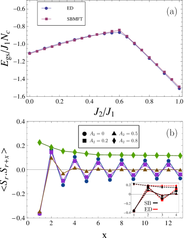
Figure 2: (a): GS energy per unit cell for $S=\frac{1}{2}$ as a function of $J_{2}/J_{1}$ for a lattice of 32 sites. The circles are exact results (ED) and the squares are the SBMFT results. (b): Spin-Spin correlation function (SSCF) vs distance ${\bf X}$ in the zig-zag direction obtained within SBMFT for a $32\times 32$ system in nos . For $0<J_{2}/J_{1}<0.41$, the SSCF correspond to the Néel phase with long-rage-order (LRO), for $0.41<J_{2}/J_{1}<0.6$ the correlations are short ranged indicating a gap zone with sort-range-order (SRO), and for $0.6<J_{2}/J_{1}$ the correlations correspond to the collinear phase (ferromagnetic correlations in the zig-zag direction). The inset in Fig. (b) shows the finite size results for the SSCF obtained by ED and SBMFT for 32 sites. Lines are guides to the eye and different colors are used for clarity.

In term of the original bosonic operators, the mean field parameters are

$$A_{\alpha\beta}(\mathbf{R})\!\! = \!\!\frac{1}{2N_{c}}\sum_{\mathbf{k}}\left\{e^{i\mathbf{k}(\mathbf{R}+\mathbf{r}_{\alpha}-\mathbf{r}_{\beta})}\langle\hat{b}^{(\alpha)}_{\mathbf{k}\uparrow}\hat{b}^{(\beta)}_{-\mathbf{k}\downarrow}\rangle\right.$$ (34)

$$- \left.e^{-i\mathbf{k}(\mathbf{R}+\mathbf{r}_{\alpha}-\mathbf{r}_{\beta})}\langle\hat{b}^{(\alpha)}_{-\mathbf{k}\downarrow}\hat{b}^{(\beta)}_{\mathbf{k}\uparrow}\rangle\right\}$$

$$B_{\alpha\beta}(\mathbf{R})\!\! = \!\!\frac{1}{2N_{c}}\sum_{\mathbf{k}}\left\{e^{i\mathbf{k}(\mathbf{R}+\mathbf{r}_{\alpha}-\mathbf{r}_{\beta})}\langle\hat{b}^{{\dagger}(\beta)}_{\mathbf{k}\uparrow}\hat{b}^{(\alpha)}_{\mathbf{k}\uparrow}\rangle\right.$$ (35)

$$- \left.e^{-i\mathbf{k}(\mathbf{R}+\mathbf{r}_{\alpha}-\mathbf{r}_{\beta})}\langle\hat{b}^{{\dagger}(\beta)}_{-\mathbf{k}\downarrow}\hat{b}^{(\alpha)}_{-\mathbf{k}\downarrow}\rangle\right\}$$

and the constraint in the number of bosons can be written in the momentum space as

$$\sum_{\mathbf{k}}\left\{\langle\hat{b}^{{\dagger}(\alpha)}_{\mathbf{k}\uparrow}\hat{b}^{(\alpha)}_{\mathbf{k}\uparrow}\rangle+\langle\hat{b}^{{\dagger}(\alpha)}_{-\mathbf{k}\downarrow}\hat{b}^{(\alpha)}_{-\mathbf{k}\downarrow}\rangle\right\}=2SN_{c},$$ (36)

where $N_{c}$ is the total number of unit cells and $S$ is the spin strength. The mean field equations (34) and (35) must be solved in a self-consistent way together with the constraints (36) on the number of bosons. Finding numerical solutions involves finding the roots of 24 coupled nonlinear equations for the parameters $A$ and $B$, plus the additional constraints to determine the values of the Lagrange multipliers $\lambda^{(\alpha)}$. We perform the calculations for finite but very large lattices and finally we extrapolate the results to the thermodynamic limit. We solve numerically for several values of the frustration parameter $J_{2}/J_{1}$ and with the values obtained for the MF parameters and the Lagrange multipliers we compute the energy and the new values for the MF parameters. We repeat this self-consistent procedure until the energy and the MF parameters converge. After reaching convergence we can compute all physical quantities like the energy, the spin-spin correlations and the excitation gap. In order to support the analytical results of the MF approach, we have also performed exact diagonalization on finite systems with 18, 24 and 32 spins with periodic boundary conditions for $S=1/2$ using Spinpack spinpack .

III Results

In Fig. 2(a) we show the ground state energy per unit cell as a function of the frustration for a system of 32 sites calculated by means of SBMFT and ED, showing an excellent agreement between both approaches. The advantage of the SBMFT is that it allows to study much larger systems: we have studied different system sizes up to 3200 sites and extrapolated to the thermodynamic limit.

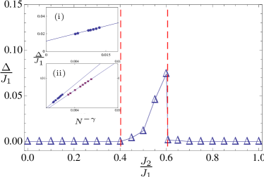
Figure 3: Gap in the boson dispersion as a function of $J_{2}/J_{1}$ for $S=1/2$ from Ref. nos . In the region $J_{2}/J_{1}\sim 0.6$ the system remains gapped. Inset: finite size scaling for the gap. (i) $J_{2}/J_{1}=0.5$ ($\gamma=0.6451$), (ii): Circles correspond to $J_{2}/J_{1}=0.05$ ($\gamma=0.911$) and squares correspond to $J_{2}/J_{1}=0.35$ ($\gamma=0.758$).

For the present model we only find commensurate collinear phases and for these phases, the wave vector $\mathbf{Q}_{0}={\bf Q}/2$ where the dispersion relation has a minimum remains pinned at a commensurate point in the Brillouin zone, independently of the value of the frustration $J_{2}/J_{1}$. In the thermodynamic limit, a state with LRO is characterized in the Schwinger boson approach by a condensation of bosons at the wave vector ${\bf Q}_{0}$. This implies that the dispersion of the bosons in a state with LRO is gapless. As we discussed earlier, we solve the mean field equations for finite systems, then to detect LRO we calculate the gap in the bosonic spectrum as a function of $J_{2}/J_{1}$ for different system sizes and perform a finite size scaling finding a finite region where the system remains gapped.

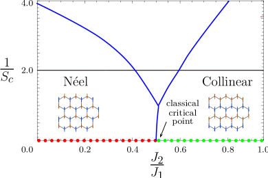
Figure 4: (Color online) Inverse of the critical spin $S_{c}$ as a function of $J_{2}/J_{1}$ obtained using SBMFT by us in nos . For the $S=1/2$ case, there is a range $0.41<J_{2}/J_{1}<0.6$ where the system has a spin-gap indicating a quantum disordered phase (see Fig. 3). The dotted-line correspond to the classical limit $S\to\infty$ where the ground state correspond to the Neel phase with $\mathbf{Q}=(0,0)$ and $\phi_{A}-\phi_{B}=\pi$ in the region $J_{2}/J_{1}<0.5$, while for $J_{2}/J_{1}>0.5$ the ground state correspond to the CAF phase characterized by $\mathbf{Q}=(2\pi/\sqrt{3},0)$ and $\phi_{A}-\phi_{B}=\pi$.

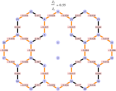
Figure 5: Dimer-dimer correlations $D_{(1,2),(k,l)}$ between the reference bond $\left(1,2\right)$ and bonds $\left(k,l\right)$ in the ground-state of the $N=24$ sample for $J_{2}/J_{1}=0.55$. The number on bond $\left(k,l\right)$ indicates the value of $D_{(1,2),(k,l)}$ truncated to the two first significant digits. Full black (orange) lines indicate positive (negative) values of $D_{(1,2),(k,l)}$.

The structure of the different phases can be understood calculating the spin-spin correlation function (SSCF).
For $J_{2}/J_{1}<0.41$ the SSCF is antiferromagnetic in all directions and is long-ranged while for $0.6<J_{2}/J_{1}$ we have found ferromagnetic LRO correlations in the zig-zag direction that correspond to the CAF phase. The most interesting result is in the intermediate region $0.41<J_{2}/J_{1}<0.6$ where the results for the SSCF predict a quantum disordered state with a gap in the bosonic dispersion and the spin-spin correlation function shows Néel short range order. A plot of the SSCF for $J_{2}/J_{1}=0,0.2,0.5$ and $0.8$ obtained within SBMFT is presented in Fig. 2b. In Fig. 4 we show the ground state phase diagram as a function of $1/S$ nos . The classical phase diagram reduces to that shown in the line $1/S_{c}=0$ of Fig. 4 where two collinear phases meet at the classical critical point $J_{2}/J_{1}=0.5$. On the one hand, for $1/S$ smaller than a critical value $1/Sc(J_{2}/J_{1})$, the correlation functions have LRO, characterized by a condensation of bosons at the wave vector ${\bf Q}_{0}$. On the other hand, when $1/S$ is greater than $1/Sc(J_{2}/J_{1})$, the correlation functions have SRO indicating quantum disorder.
In the intermediate region the results found with SBMFT predict a quantum disordered region $0.41<J_{2}/J_{1}<0.6$. In this region a gap opens in the bosonic dispersion and the spin-spin correlation function shows Néel short range order followed by the LRO CAF phase for $J_{2}/J_{1}>0.6$. In Fig. 3 we show the extrapolation of the boson gap as a function of the frustration. The inset shows an example of the finite size scaling for different values of the frustration.

Previous results show that for $0.41<J_{2}/J_{1}<0.6$ the ground state has no magnetic order nos . The main question now is: Is this non magnetic quantum phase a quantum disordered one? Or does it exhibit any other kind of non-magnetic order?. To answer this question the knowledge of the spin-spin correlation function is not enough and one has to check for other types of (non-magnetic) ordering patterns.

One kind of non magnetic order that can set in is the dimer long-range order. The dimer operator on a pair of sites $\left(i,j\right)$ is defined as $\hat{\bf d}_{i,j}=1/4-\hat{\bf S}_{i}\cdot\hat{\bf S}_{j}$, and one usually defines the dimer-dimer correlation between bonds $(i,j)$ and $(k,l)$ as $D_{(i,j),(k,l)}=<\hat{\bf d}_{i,j}\hat{\bf d}_{k,l}>-<\hat{\bf d}_{i,j}><\hat{\bf d}_{k,l}>$. In order to understand the nature of the ground state in the intermediate region, we have calculated de dimer-dimer correlation function defined above by means of exact diagonalization on a 24 sites cluster with periodic boundary conditions for $S=1/2$. The correlation pattern for dimers on first neighbor bonds is displayed in Fig. 5. We can see that the exact dimer-dimer correlations show a rather fast decay suggesting that there is no dimer order in the groud state, though due to the small size of the cluster studied, this is not conclusive and we cannot discard other ordering patterns.

In summary, the results presented here further support the existence of a region in the intermediate frustration regime where the system does not show quantum magnetic order for $S=1/2$.

Note added: When this manuscript was completed we became aware of two independent works providing an analysis of the model using a combination of exact diagonalizations Farnell ; Capponi and an effective quantum dimer model, as well as a self-consistent cluster mean-field theory Capponi . Several similar findings show a good correspondence of both approaches.

Acknowledgements: This work was partially supported by the ESF grant INSTANS, PICT ANPCYT (Grant No 2008-1426) and PIP CONICET (Grant No 1691).