Analysis of Longitudinal Air Shower Profiles measured by the Pierre Auger Observatory

Abstract

We describe the analysis of longitudinal air shower profiles as measured by the fluorescence detectors of the Pierre Auger Observatory and present the measurement of the depth of maximum of extensive air showers, ${X_{\mathrm{max}}}$, with energies $\geq$ $10^{18}$ eV . The measured energy evolution of the average of ${X_{\mathrm{max}}}$ and its fluctuations, RMS$(X_{\mathrm{max}})$, are compared to air shower simulations for different primary particles.

1 Introduction

The determination of the chemical composition of ultra-high energy cosmic rays is essential to understand the origin of cosmic rays and to interpret the features observed in the ultra-high energy cosmic ray flux. For instance, the observed hardening of the cosmic ray energy spectrum at energies between $10^{18}$ eV and $10^{19}$ eV , known as the ’ankle’, might either be a signature of the transition from galactic to extragalactic cosmic rays or a distortion of a proton-dominated extragalactic spectrum due to energy losses ankle . Moreover, the flux suppression observed above 4$\cdot$$10^{19}$ eV  bib:gzkmeas could be either due to propagation effects bib:gzk (photopion production of primary protons or photonuclear reactions of primary nuclei) or a signature of the maximum injection energy of the sources maxEnergy .

There are several experimental methods to estimate the primary composition from cosmic ray induced air showers. Within the Pierre Auger Observatory (see bib:auger and bib:bruce ) the observation of the longitudinal shower development with fluorescence detectors allows to measure the depth of the maximum of the shower evolution, ${X_{\mathrm{max}}}$, which is sensitive to the primary mass.

With the generalization of Heitler’s model of electron-photon cascades to hadron-induced showers bib:heitlerModel and the superposition assumption for nuclear primaries of mass $A$, the average depth of the shower maximum, $\langle X_{\mathrm{max}}\rangle$, at a given energy $E$ is expected to follow

$${\langle X_{\mathrm{max}}\rangle}=\alpha\left(\ln E-\langle\ln A\rangle\right)+\beta,$$ (1)

where $\langle\ln A\rangle$ is the average of the logarithm of the primary masses. The coefficients $\alpha$ and $\beta$ depend on the nature of hadronic interactions, most notably on the multiplicity, elasticity and cross-section in ultra-high energy collisions of hadrons with air, see e.g. Ulrich:2009hm . The change of $\langle X_{\mathrm{max}}\rangle$ per decade of energy is called elongation rate bib:elongationRate , $D_{10}=\frac{\mathrm{d}{\langle X_{\mathrm{max}}\rangle}}{\rm{d}\lg E}$, and it is sensitive to changes in composition with energy. A complementary composition-dependent observable is the magnitude of the shower-to-shower fluctuations of the depth of maximum, RMS$(X_{\mathrm{max}})$, which is expected to decrease with the number of primary nucleons $A$ (though not as fast as $1/\sqrt{A}$

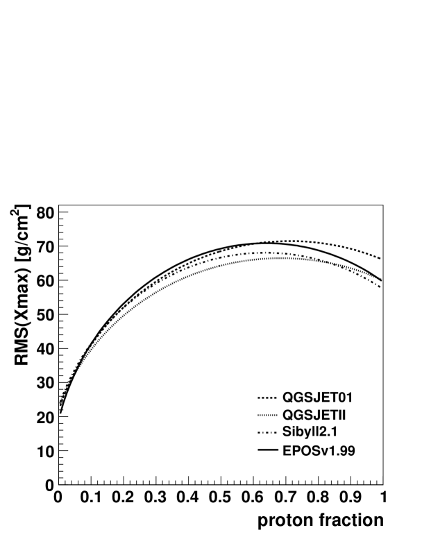
Figure 1: RMS$(X_{\mathrm{max}})$ from different hadronic interaction models bib:simulations and a two-component p/Fe composition model ($E=$$10^{18}$ eV ).

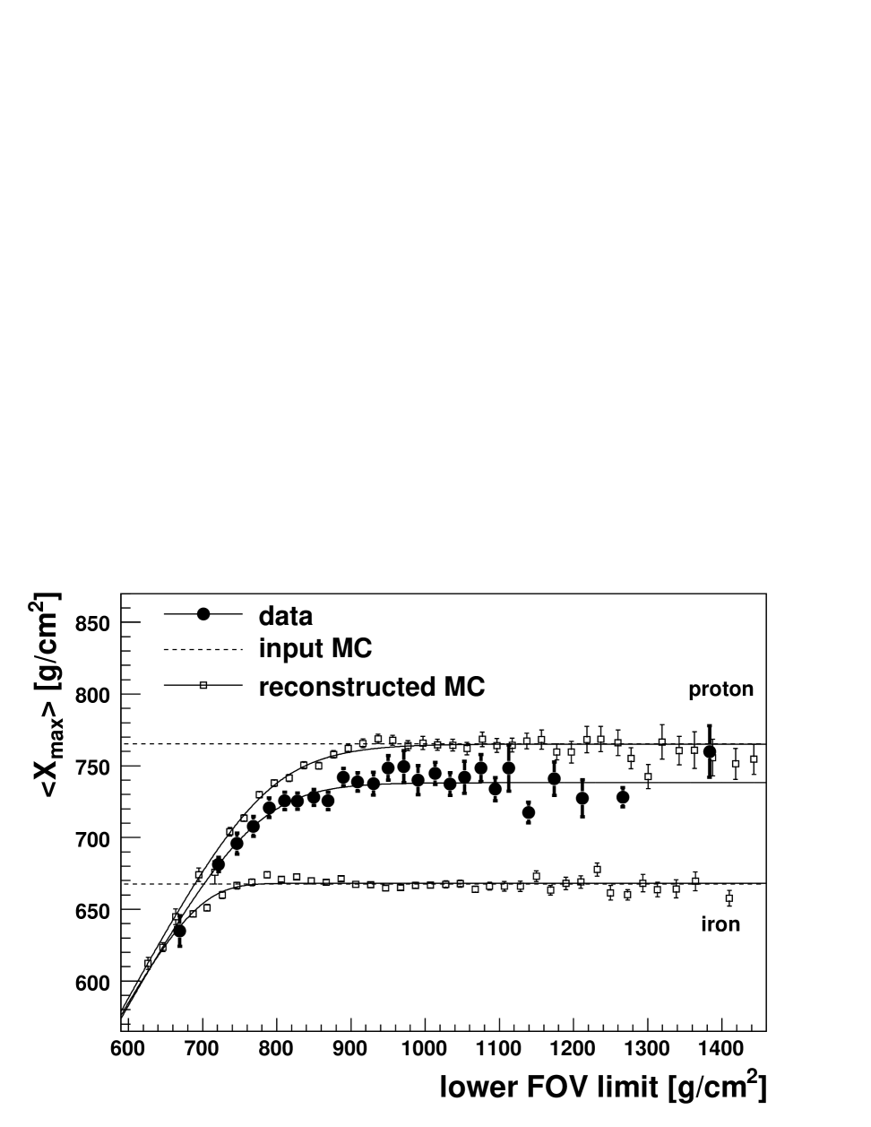
Figure 2: Left: Illustration of the field of view bias. Right: Dependence of $\langle X_{\mathrm{max}}\rangle$ on the field of view boundary close to ground for data and MC ($10^{18.4}$ eV $<E<$$10^{18.6}$ eV ).

bib:fluctuations ) and to increase with the interaction length of the primary particle. In case of a mixed composition, the full width of the $X_{\mathrm{max}}$ distribution follows from the shower-to-shower fluctuations of the individual mass groups and their separation in $\langle X_{\mathrm{max}}\rangle$ bib:linsleyCompo . For a simple two-component composition of primaries with masses $A_{1}$ and $A_{2}$ and abundances $f_{1}$ and $f_{2}=(1-f_{1})$, RMS$(X_{\mathrm{max}})$ is given by

$${\mathrm{RMS}(X_{\mathrm{max}})}=\left(f_{1}V_{1}+f_{2}V_{2}+f_{1}f_{2}\Delta_{X}^{2}\right)^{\frac{1}{2}}$$ (2)

where $V_{i}={\mathrm{RMS}(X_{\mathrm{max}})}_{i}^{2}$ and $\Delta_{X}={\langle X_{\mathrm{max}}\rangle}_{1}-{\langle X_{\mathrm{max}}\rangle}_{2}$. As can be seen in Fig. 1, a proton/iron mixture gives rise to a broad maximum in RMS$(X_{\mathrm{max}})$ for $0.3\lesssim f_{\mathrm{p}}\lesssim 1$ and a rapid decrease of the width towards $f_{\mathrm{p}}=0$.

2 Data Analysis

The ${X_{\mathrm{max}}}$ results which were discussed at this workshop are based on bib:Abraham:2010yv and use air shower data recorded between December 2004 and March 2009. Only events detected in hybrid mode bib:hybrid are considered, i.e. the shower development must have been measured by the fluorescence detector (FD), and at least one coincident surface detector station is required to provide a ground-level time. Using the time constraint from the surface detector, the shower geometry can be determined with an angular uncertainty of 0.6^∘ bib:angReso . The longitudinal profile of the energy deposit is reconstructed bib:profileRec from the light recorded by the FD using the fluorescence and Cherenkov yields and lateral distributions from bib:lightyields . With the help of data from atmospheric monitoring devices bib:augeratmo the light collected by the telescopes is corrected for the attenuation between the shower and the detector and the longitudinal shower profile is reconstructed as a function of atmospheric depth. $X_{\mathrm{max}}$ is determined by fitting the reconstructed longitudinal profile with a Gaisser-Hillas function bib:gaisser-hillas .

To assure a good ${X_{\mathrm{max}}}$ resolution, the following quality cuts are applied: The impact of varying atmospheric conditions on the $X_{\mathrm{max}}$ measurement is minimized by rejecting time periods with cloud coverage and by requiring reliable measurements of the vertical optical depth of aerosols. Profiles that are distorted by residual cloud contamination are rejected by a loose cut on the quality of the profile fit ($\chi^{2}$/Ndf$<$2.5). We take into account events only with energies above $10^{18}$ eV where the probability for at least one triggered surface detector station is 100%, irrespective of the mass of the primary particle bib:hybridExposure . The geometrical reconstruction of showers with a large apparent angular speed of the image in the telescope is susceptible to uncertainties in the time synchronization between the fluorescence and surface detector. Therefore, events with a light emission angle towards the FD that is smaller than 20^∘ are rejected. This cut also removes events with a large fraction of Cherenkov light. The energy and shower maximum can be reliably measured only if $X_{\mathrm{max}}$ is in the field of view (FOV) of the telescopes (covering $1.5^{\circ}$ to $30^{\circ}$ in elevation). Events for which only the rising or falling edge of the profile is detected are not used. Moreover, we calculate the expected statistical uncertainty of the reconstruction of $X_{\mathrm{max}}$ for each event, based on the shower geometry and atmospheric conditions, and require it to be better than 0pt40.

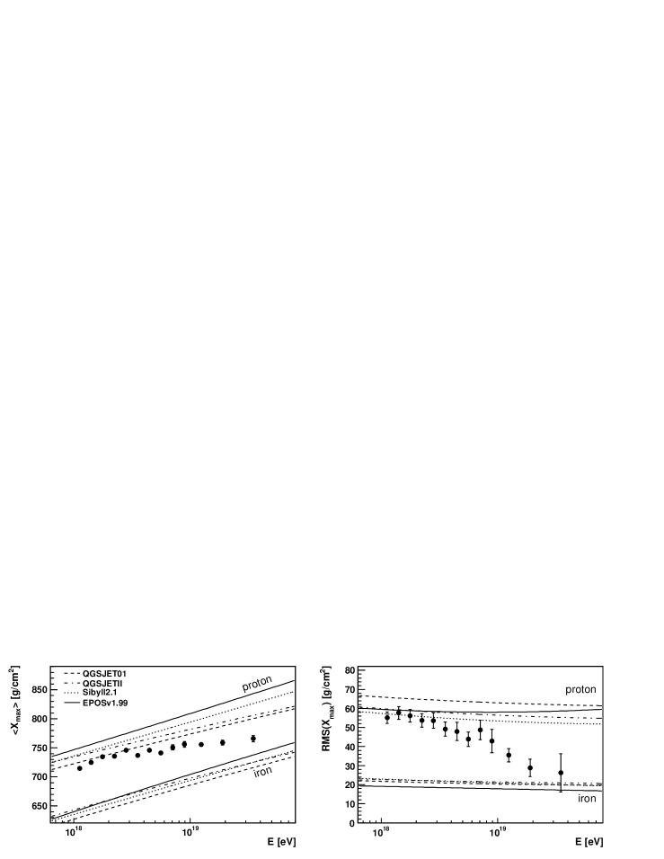
Figure 3: $\langle X_{\mathrm{max}}\rangle$ and RMS$(X_{\mathrm{max}})$ compared with air shower simulations bib:conex using different hadronic interaction models bib:simulations .

The latter two selection criteria may cause a systematic under-sampling of the tails of the $X_{\mathrm{max}}$ distribution, since showers developing very deep or shallow in the atmosphere might be rejected from the data sample (see illustration in the left panel of Fig. 2). To avoid a corresponding bias in the measured $\langle X_{\mathrm{max}}\rangle$ and RMS$(X_{\mathrm{max}})$ we apply fiducial volume cuts on the viewable $X_{\mathrm{max}}$ range. For this purpose the effective upper and lower field of view limits are calculated for each event and $\langle X_{\mathrm{max}}\rangle$ is measured as a function of these limits. An example of the $\langle X_{\mathrm{max}}\rangle$ dependence on the lower FOV limit is shown in Fig. 2 for data and simulated events. As can be seen, the $\langle X_{\mathrm{max}}\rangle$ is asymptotically unbiased for events with a sufficiently deep FOV limit, but it is systematically too shallow when the FOV boundary starts cutting into the tails of the $X_{\mathrm{max}}$ distribution. Obviously, the unbiased region depends on the distribution itself and can thus not be determined by simulations. Instead, we fit the data with the mean of a one-sided truncated normal distribution (shown as solid lines in Fig. 2) and reject all events that have a FOV limit for which the measured $\langle X_{\mathrm{max}}\rangle$ departs by more than 0pt5 from its asymptotic value.

After all cuts, 3754 events are selected for the $X_{\mathrm{max}}$ analysis. The $X_{\mathrm{max}}$ resolution as a function of energy for these events is estimated using a detailed simulation of the FD and the atmosphere. The resolution, defined by the full standard deviation, is at the 0pt20 level above a few EeV. The difference between the reconstructed $X_{\mathrm{max}}$ values in events that had a sufficiently high energy to be detected independently by two or more FD stations is used to cross-check these findings and as it was shown in bib:Abraham:2010yv , the simulations reproduce the data well.

3 Results

The measured $\langle X_{\mathrm{max}}\rangle$ and RMS$(X_{\mathrm{max}})$ are measured in energy bins of $\Delta\lg E=0.1$ below 10 EeV and $\Delta\lg E=0.2$ above that energy. The last bin starts at $10^{19.4}$ eV , integrating up to the highest energy event ($E=(59\pm 8)$ EeV). The systematic uncertainty of the FD energy scale is 22% bib:icrcflux . Uncertainties of the calibration, atmospheric conditions, reconstruction and event selection give rise to a systematic uncertainty of $\leq$0pt13 for ${\langle X_{\mathrm{max}}\rangle}$ and $\leq$0pt6 for the RMS. The results were found to be independent of zenith angle, time periods and FD stations within the quoted uncertainties.

The measured values are displayed in Fig. 3. A fit of ${\langle X_{\mathrm{max}}\rangle}$ data with a constant elongation rate does not describe our data ($\chi^{2}$/Ndf=34.9/11), but using two slopes yields a satisfactory fit ($\chi^{2}$/Ndf=9.7/9) with an elongation rate of (106${}^{+35}_{-21}$) g/cm²/decade below $10^{18.24\pm 0.05}$ eV and (24$\pm$3) g/cm²/decade above this energy. If the properties of hadronic interactions do not change significantly over less than two orders of magnitude in primary energy ($<$ factor 10 in center of mass energy), this change of $\Delta D_{10}=$$(82^{+35}_{-21})$ g/cm²/decade would imply a change in the energy dependence of the composition around the ankle, supporting the hypothesis of a transition from galactic to extragalactic cosmic rays in this region.

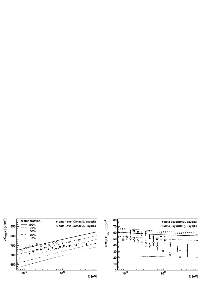
Figure 4: $\langle X_{\mathrm{max}}\rangle$ and RMS$(X_{\mathrm{max}})$ compared to QgsjetII predictions for a two-component iron/proton composition. Data points show extreme values obtained by shifting the measurements by $\pm$ one sigma of the systematic uncertainties.

The shower-to-shower fluctuations, RMS$(X_{\mathrm{max}})$, are obtained by subtracting the detector resolution in quadrature from the width of the observed $X_{\mathrm{max}}$ distributions resulting in a correction of $\leq$0pt6. As can be seen in the right panel of Fig. 3, we observe a decrease in the fluctuations with energy from about 55 to 0pt26 as the energy increases. Assuming again that the hadronic interaction properties do not change much within the observed energy range, these decreasing fluctuations are an independent signature of an increasing average mass of the primary particles.

For the interpretation of the absolute values of $\langle X_{\mathrm{max}}\rangle$ and RMS$(X_{\mathrm{max}})$ a comparison to air shower simulations is needed. As can be seen in Fig. 3, there are considerable differences between the results of calculations using different hadronic interaction models. These differences are not necessarily exhaustive, since the hadronic interaction models do not cover the full range of possible extrapolations of low energy accelerator data. If, however, taken at face value, the comparison of the data and simulations leads to the same conclusions as above, namely a gradual increase of the average mass of cosmic rays with energy up to 59 EeV.

It is illustrative to compare the data with predictions for a simple two-component proton/iron model using the QgsjetII hadronic interaction model. ${\langle X_{\mathrm{max}}\rangle}$ and ${\mathrm{RMS}(X_{\mathrm{max}})}$ simulations for different proton fractions $f$ are shown in Fig.4. As can be seen, the ${\langle X_{\mathrm{max}}\rangle}$ values change linearly with $f$ as expected from Eq. (1), whereas the width of the ${X_{\mathrm{max}}}$ distribution is very similar for proton fractions $f\gtrsim 0.3$. To visualize the systematic uncertainties of the data, in this figure we shifted the default results from Fig. 3 by their systematic uncertainties. Note that the systematics on ${\mathrm{RMS}(X_{\mathrm{max}})}$ are dominated by the event selection, whereas the systematics on ${\langle X_{\mathrm{max}}\rangle}$ are mainly due to reconstruction uncertainties and atmospheric effects. Therefore sys$({\langle X_{\mathrm{max}}\rangle})$ and sys$(\mathrm{RMS})$ are uncorrelated and can be shifted independently. Within this simplistic two-component model, the data is compatible with a light or mixed composition at low energies. At high energies, a heavy composition would result, but the ${\langle X_{\mathrm{max}}\rangle}$ would indicate a larger proton fraction than ${\mathrm{RMS}(X_{\mathrm{max}})}$. At high energies, this model corresponds to a heavy composition, however, the ${\langle X_{\mathrm{max}}\rangle}$ would indicate a larger proton fraction than ${\mathrm{RMS}(X_{\mathrm{max}})}$.

References

- (1) A.M. Hillas, Phys. Lett. 24, 677; V.S. Berezinsky and S.I. Grigor’eva, Astron. Astrophys. 199 (1988) 1; D. Allard, E. Parizot and A. V. Olinto, Astropart. Phys. 27 (2007) 61; R. Aloisio, V. Berezinsky, P. Blasi and S. Ostapchenko, Phys. Rev. D 77 (2008) 025007.
- (2) R. Abbasi et al. [HiRes Coll.], Phys. Rev. Lett. 100 (2008), 101101; J. Abraham et al. [Pierre Auger Coll.], Phys. Rev. Lett. 101 (2008), 061101; J. Abraham et al. [Pierre Auger Coll.], Phys. Lett. B 685, (2010) 239.
- (3) K. Greisen, Phys. Rev. Lett. 16 (1966), 748; G.T. Zatsepin and V.A. Kuzmin, JETP Lett. 4 (1966), 78.
- (4) D. Allard et al., JCAP 0810 (2008) 033, R. Aloisio et al., Astropart. Phys. 34 (2011), 620.
- (5) J. Abraham et al. [Pierre Auger Coll.], Nucl. Instrum. Meth. A523 (2004), 50; I. Allekotte et al. [Pierre Auger Coll.], Nucl. Instrum. Meth. A 586 (2008) 409. J. Abraham et al. [Pierre Auger Coll.], Nucl. Instr. Meth. A620 (2010), 227;
- (6) B.R. Dawson for the Pierre Auger Coll., these proceedings.
- (7) J. Abraham et al. [Pierre Auger Coll.], Proc. 31st ICRC (2009), arXiv:0906.2319.
- (8) W. Heitler, Oxford University Press, 1954; J. Matthews, Astropart. Phys. 22 (2005), 387.
- (9) T. Wibig, Phys. Rev. D 79 (2009), 094008; R. Ulrich et al., Phys. Rev. D bf 83 (2011), 054026; R. D. Parsons et al., arXiv:1102.4603.
- (10) J. Linsley, Proc. 15th ICRC 12 (1977), 89; T.K. Gaisser et al., Proc. 16th ICRC 9 (1979), 258; J. Linsley and A.A. Watson, Phys. Rev. Lett. 46 (1981), 459.
- (11) J. Engel et al., Phys. Rev. D46 (1992), 5013.
- (12) J. Linsley, Proc. 18th ICRC 12 (1983), 135.
- (13) J. Abraham et al. [Pierre Auger Coll.], Phys. Rev. Lett. 104 (2010), 091101.
- (14) P. Sommers, Astropart. Phys. 3 (1995), 349; B.R. Dawson et al., Astropart. Phys. 5 (1996), 239.
- (15) C. Bonifazi et al. [Pierre Auger Coll.], Nucl. Phys. Proc. Suppl. 190 (2009) 20, arXiv:0901.3138.
- (16) M. Unger et al., Nucl. Instrum. Meth. A588 (2008), 433;
- (17) M.D. Roberts, J. Phys. G 31 (2005), 1291; D. Gora et al., Astropart. Phys. 24 (2006), 484; F. Nerling et al., Astropart. Phys. 24 (2006), 421; B.R. Dawson, M.Giller and G. Wieczorek, Proc. 30th ICRC (2007); B. Keilhauer et al., Nucl. Instrum. Meth. A597, (2008) 99.
- (18) J. Abraham et al. [Pierre Auger Coll.], Astropart. Phys. 33 (2010) 108; J. Abraham et al. [Pierre Auger Coll.], Astropart. Phys. 32 (2009) 89.
- (19) T.K. Gaisser and A.M. Hillas, Proc. 15th ICRC, 8, 353 (1977).
- (20) P. Abreu et al. [Pierre AugerColl.], Astropart. Phys. 34 (2011) 368-381.
- (21) M. Unger [Pierre Auger Coll.], Nucl. Phys. Proc. Suppl. 190 (2009) 240 [arXiv:0902.3787]; J.A. Bellido [Pierre Auger Coll.], Proc. XXth Rencontres de Blois (2008) [arXiv:0901.3389]
- (22) T. Bergmann et al., Astropart. Phys. 26 (2007) 420.
- (23) N.N. Kalmykov and S.S. Ostapchenko, Phys. Atom. Nucl. 56 (1993), 346; S.S. Ostapchenko, Nucl. Phys. Proc. Suppl. 151 (2006), 143; T. Pierog and K. Werner, Phys. Rev. Lett. 101 (2008), 171101; E. -J. Ahn et al., Phys. Rev. D80 (2009), 094003.
- (24) J. Abraham et al. [Pierre Auger Coll.], Proc. 31st ICRC (2009), arXiv:0906.2189.