Anomalous Magnetic Susceptibility and Hall Effect from Valley Degrees of Freedom

Abstract

We study the magnetic and transport properties of epitaxial graphene films in this letter. We predict enhanced signal of magnetic susceptibility and relate it to the intrinsic valley magnetic moments. There is also an anomalous contribution to the ordinary Hall effect, which is due to the valley dependent Berry phase or valley-orbit coupling.

Graphene, a monolayer carbon honeycomb lattice, has extraordinary electronic properties[1,2]. Its conduction band and valence band form conically shaped valleys, touching at two nonequivalent corners of the hexagonal Brillouin zone called Dirac points. For optical and electronic application, it is desirable to make graphene semiconducting by opening a gap. A gap can be produced either by size quantization effects in graphene nano-ribbons[3], or by inversion symmetry breaking for epitaxial graphene grown on the top of crystals with matching lattices such as BN or SiC [4]. For the latter case, a significant energy gap has been predicted from ab initio calculation[5], although the experimental evidence for the gap is still under debate[6]. Experimentally, epitaxial graphene is relatively disordered and heavily doped because of close contact with the substrate. However, interesting physics can still manifest due to robust topological effects associated with the valley degree of freedom.

In this Letter, we present our studies of magnetic and transport properties of epitaxial graphene systems. It is assumed that the interaction between the graphene layer and the substrate breaks the sublattice symmetry, which opens up a band gap at Dirac points[6]. We predict enhanced signals of magnetic susceptibility and anomalous contribution to the ordinary Hall effect. It is demonstrated that these extroadinary effects are due to the special valley degree of freedom in the system. Furthermore, we argue that both effects are robust against disorder, hence should be readily detected in experiment.

Magnetic susceptibility. Recent studies on the orbital magnetism of 2D massless Dirac fermions have shown that the unique Landau-level structure gives rise to a singular diamagnetism[7]. The susceptibility becomes highly diamagnetic when the chemical potential is at band-touching point ($\mu$=0 eV) where the density of states vanishes,

$$\chi_{0}\left(\mu\right)=-\frac{{e^{2}a^{2}t^{2}}}{{4\pi\hbar^{2}}}\frac{\beta}{(e^{\beta\mu/2}+e^{-\beta\mu/2})^{2}}.$$ (1)

Here, t is the nearest neighbor hopping energy, a is the lattice constant and $\beta=1/k_{B}T$. $T$ is the temperature and $k_{B}$ is the Boltzman constant. It is still mysterious about the mechanism of such a singular behavior. A natural question is what happens to the susceptibility when a finite gap opens at the Dirac points.

With a staggered sublattice potential, the low-energy effective Hamiltonian near the Dirac points is given by[8,9]

$$H = \left[\begin{array}[]{cc}\frac{\Delta}{2}&v_{0}\left(\Pi_{x}\tau_{z}-i\Pi_{y}\right)\\ v_{0}\left(\Pi_{x}\tau_{z}+i\Pi_{y}\right)&-\frac{\Delta}{2}\end{array}\right],$$

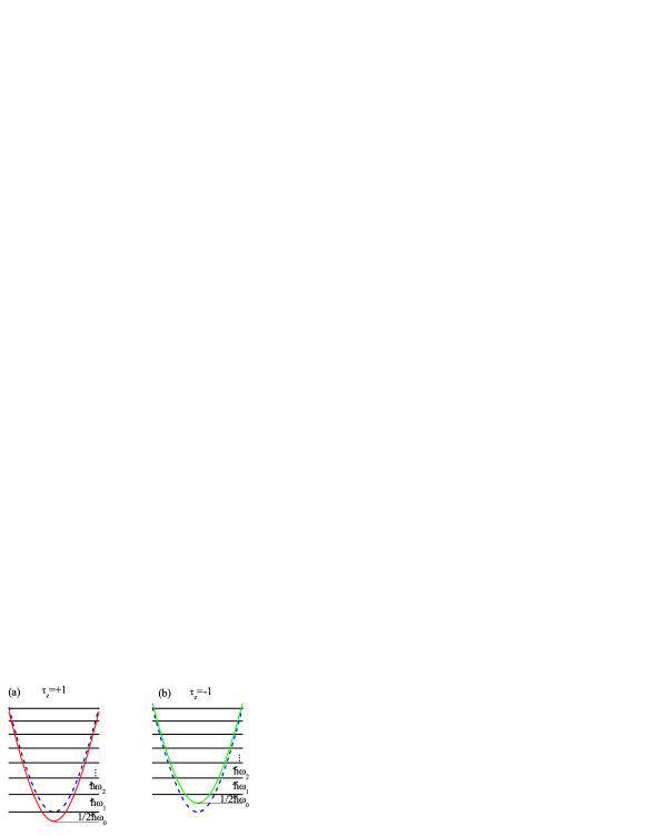
Figure 1: (Color online). The Landau levels from exact quantum calculations for $\tau_{z}=+1$ (a) and $\tau_{z}=-1$ (b) valleys. For comparison, the energy dispersions $\varepsilon_{0}(\textbf{k})$ (dashed line) and $\varepsilon(\textbf{k})=\varepsilon_{0}(\textbf{k})-\textbf{m}(\textbf{k})\cdot\textbf{B}$ (solid curves) are shown. Parameters are $\Delta$= 0.28 $eV$, $t$= 2.82 $eV$ and lattice constant $a$=2.46 Ȧ.

where $v_{0}=\sqrt{3}at/2$ and $\Pi\equiv\textbf{k}+e\textbf{A}$ is the reduced momentum operator in a magnetic field. $\Delta$ is the site energy difference between sublattices, which also corresponds to the band gap. From commutation relation [$\Pi_{\pm},\Pi_{\mp}$]=$\mp 2eB/\hbar$ where $\Pi_{\pm}=\Pi_{x}\pm i\Pi_{y}$, we define ladder operators $b$ and $b^{\dagger}$ such that: $\Pi_{+}=(\sqrt{2eB/\hbar})b^{{\dagger}}$ and $\Pi_{-}=(\sqrt{2eB/\hbar})b$. The wave function is constructed from the linear combination of eigenstates $|n\rangle$ of operator $b$. The Hamiltonian (2) is diagonalized to yield the Landau levels, which in conduction band is shown in Fig.1:

$$\varepsilon_{n}(\tau_{z})=\left\{{\begin{array}[]{*{20}c}{\tau_{z}\frac{\Delta}{2}\hfill}&{(n=0),\hfill}\\ {\pm\sqrt{\left({\frac{\Delta}{2}}\right)^{2}+\frac{{3a^{2}t^{2}eB}}{{2\hbar}}n}\hfill}&{(n=1,2\cdots).\hfill}\\ \end{array}}\right.$$ (3)

where $\tau_{z}=\pm 1$ labels the two valleys.

The magnetic susceptibility is defined as $\chi\equiv-\left({\frac{{\partial^{2}F}}{{\partial B^{2}}}}\right)_{\mu}$, where the thermodynamic potential can be calculated from the formula $F=-\frac{1}{\beta}\frac{{eB}}{h}\sum\limits_{n,\tau_{z}}{\ln\left[{1+e^{\beta(\mu-\varepsilon_{n})}}\right]}$. By using the Euler-Maclaurin formula, we get the expand $F$ as a power series with respect to $B$ and the analytical expression of susceptibility is [10]

$$\chi(\mu)=-\frac{{e^{2}a^{2}t^{2}}}{{4\pi\hbar^{2}\Delta}}\frac{{e^{\beta\mu}\left({e^{\beta\Delta/2}-e^{-\beta\Delta/2}}\right)}}{{1+2e^{\beta\mu}\textrm{Cosh}(\beta\Delta/2)+e^{2\beta\mu}}}.$$ (4)

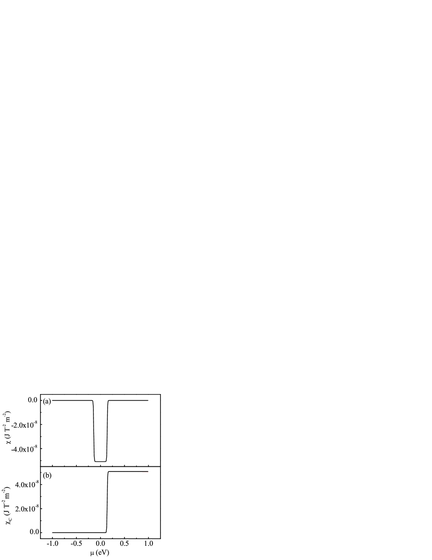
Figure 2: (Color online). (a) Magnetic susceptibility as a function of chemical potential. (b) Magnetic susceptibility from conduction electrons only. Here, $T=$ 10 $K$ and $\Delta$= 0.28 $eV$.

Fig.2(a) shows the numerical result of the magnetic susceptibility at $T=10$K. In the calculation we take $\Delta\sim 0.28$ $eV$, $t\sim 2.82$ $eV$ and $a=2.46$Ȧ[5]. Compared with the zero gap case, it is observed that the large diamagnetic dip is still visible even when the gap opens, and it gets broadened in energy by the gap width. Disorder effects smooth out this curve but will not change the main features because susceptibility $\chi$ is a thermodynamic property. We find that the integral of susceptibility over chemical potential, i.e. $\int{\chi(\mu)d\mu}$, is independent of both gap size and temperature. At zero temperature, the susceptibility becomes a square well shape, and vanishes when it is either electron- or hole-doped.

The sudden jump of magnetic susceptibility at band edges signifies a large paramagnetism from the carriers. Indeed, if we calculate the magnetic susceptibility from Landau levels above the gap, then the conduction band contribution to $\chi$ can be obtained as

$$\chi_{C}(\mu)=\frac{{e^{2}a^{2}t^{2}}}{{4\pi\hbar^{2}\Delta}}\frac{1}{{1+e^{-\beta(\mu-\Delta/2)}}}.$$ (5)

From the plot in Fig.2(b), we can see that the large paramagnetic response from the conduction electrons. What is the source of this paramagnetism? Note that our model does not take into account of spin degree of freedom, so it must come from the orbital motion of electrons. In fact, previous studies have shown that there is an intrinsic magnetic moment associated with the valley degree of freedom[11]. At conduction band bottom ($\mu=\Delta/2$), the moment equals the effective Bohr magneton $\mu_{B}^{*}=\tau_{z}\frac{e\hbar}{2m_{e}^{*}}$ with the effective mass $m_{e}^{*}=\frac{{2\hbar^{2}\Delta}}{{3a^{2}t^{2}}}$. If one models this system by a 2D nonrelativistic electron gas with such a pseudo-spin degree of freedom, one would obtain both Pauli paramagnetic and Landau diamagnetic contributions recovering our expression Eq(5) above.

Therefore, it is the valley magnetic moment that determines the magnitude of the susceptibility signal. Using an experimentally measured energy gap of 0.28 eV for graphene on SiC[5], the effective mass is about 30 times smaller than the bare electron mass, hence the magnetic moment is about thirty times larger than the free electron spin magnetic moment.

Semiclassical Landau levels. To further exemplify the role of the valley magnetic moment, we now closely examine the energy spectrum and analyze it via a semiclassical approach. If we place the exact Landau levels on the background of the original conduction band dispersion curve, one discovers that Landau levels from one valley start at the edge of the zero-field band (dashed curves in Fig.1), while those from the other valley start from one cyclotron energy above. The situation looks less odd if one shifts the bands by the Zeeman energy $-\textbf{m}(\textbf{k})\cdot\textbf{B}$, where $\textbf{m}(\textbf{k})=\tau_{z}\frac{{3e\Delta a^{2}t^{2}}}{{4\hbar\left({\Delta^{2}+3k^{2}a^{2}t^{2}}\right)}}$ is the valley magnetic moment[12]. Relative to the new bands (solid curves), the Landau levels of both valleys now start at half of the cyclotron energy above the band edges, which is the familiar result for 2D free electron gas.

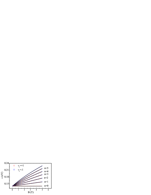
Figure 3: (Color online). The field dependence of semiclassical Landau levels for $\tau_{z}=+1$ (red circle) and $\tau_{z}=-1$ (blue triangle) valleys. For comparison, the exact quantum Landau levels are also shown (solid line).

Furthermore, one can obtain the Landau levels by semiclassically quantizing the cyclotron orbits in these modified bands. By taking into account the Berry phase correction, Onsager’s quantization condition for the areas enclosed by the cyclotron orbits becomes $\pi k^{2}=\frac{{2\pi eB}}{\hbar}[n+\frac{1}{2}-\frac{\Gamma(k)}{{2\pi}}]$[13]. In Ref.[12], the Berry curvature of the conduction band at the two valleys has been calculated to be $\Omega(\textbf{k})=\tau_{z}\frac{{3\Delta a^{2}t^{2}}}{{2(\Delta^{2}+3k^{2}a^{2}t^{2})^{3/2}}}.$ The Berry phase $\Gamma(k)$ can then be obtained by integrating the Berry curvature over the area enclosed by the orbit. The energies of the modified bands at these quantized radius of the cyclotron orbits then yield the semiclassical Landau levels. Our result is shown in Fig.3, which agrees very well with the exact Landau levels. However, we must emphasize that for the low lying Landau levels close to the band edge, the Berry phase effect is relatively less important than the Zeeman shift associated with the valley magnetic moments. The situation reverses at high energies, where the magnetic moment vanishes and the Berry phase approaches $\pi$.

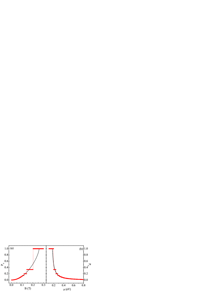
Figure 4: (Color online). (a)The variation of valley polarization $P_{V}$ with the magnetic field $B$ ($\mu$=0.2 eV). (b)The variation of valley polarization $P_{V}$ with the chemical potential $\mu$ (B=0.2 T). Both the quantum calculations (red) and semiclassical results (black) are shown.

Valley Polarization. The valley magnetic moment allows a direct coupling of the magnetic field with the valley degree of freedom. We expect that an equilibrium population difference between the two valleys can be induced by applying a magnetic field. Analogous to the spin polarization concept, we define valley polarization to be $P_{V}=(n_{+}-n_{-})/(n_{+}+n_{-})$, where $n_{\pm}$ is the densities of electrons in the valley with index $\tau_{z}=\pm 1$. This can be calculated from the relative number of occupied Landau levels in the two valleys, resulting in the series of steps shown in Fig.4. Perfect valley polarization occurs when there is one Landau level occupied in one valley but none in the other(see Fig.1).

We have also calculated the valley polarization semiclassically, in which the electron density from a given valley is obtained by integrating the Berry-curvature modified density of states up to the Fermi surface, i.e. $\int^{\mu}{\frac{d\bf k}{{(2\pi)^{2}}}}\left({1+\frac{{e\bf B\cdot\bf\Omega}}{\hbar}}\right)$[14]. The result is plotted as the black curves in Fig.4, and they smoothly go through the quantum steps. As expected, the valley polarization increases with the magnetic field (Fig.4(a)), and the induced polarization is largest at the band edge where the valley magnetic moment is largest (Fig.4(b)).

Anomalous Hall effect. It is now well established that in the presence of an in-plane electric field, an electron will acquire an anomalous velocity, proportional to the Berry curvature, in the transverse direction [13]. This leads to an intrinsic contribution to the Hall conductivity, $\sigma_{H}^{int}=2(e^{2}/\hbar)\int\frac{d^{2}k}{(2\pi)^{2}}f(k)\Omega(k)$, where $f(k)$ is the Fermi-Dirac distribution function, and the factor of 2 comes from spin degeneracy. There is also a side-jump contribution [15] proportional to the Berry curvature at the Fermi surface when carriers scatter off impurities. Ignoring skew-scattering and other effects due to inter-valley scattering, a valley-dependent Hall conductivity at zero temperature is found in Ref.[12] as $\sigma_{H}(\tau_{z})=\tau_{z}\frac{{e^{2}}}{h}\left[{1-\frac{\Delta}{{2\mu}}-\frac{\Delta(4\mu^{2}-\Delta^{2})}{{8\mu^{3}}}}\right]$. This result is independent of impurity density and strength. The valley dependence in the Hall current will lead to an accumulation of electrons on opposite sides of the sample with opposite valley indices. Clearly, if there is a net valley polarization, a charge Hall conductivity will appear upon the application of an electric field, $\sigma_{xy}=\frac{{e^{2}}}{h}\frac{\Delta}{\bar{\mu}^{2}}\left(\frac{3\Delta^{2}}{8\bar{\mu}^{2}}-1\right)\delta\mu$. Here, $\bar{\mu}$ is the chemical potential in the absence of the magnetic field, and $\delta\mu$ is the chemical potential difference between the two valleys. We can express $\delta\mu$ in terms of the field-induced valley polarization as $\delta\mu=\frac{\delta\mu}{\delta n}(n_{+}+n_{-})\frac{\partial P_{V}}{\partial B}B=\frac{2n}{D(\mu)}\frac{\partial P_{V}}{\partial B}B$, where $n$ is the electron density and $D(\mu)$ is the density of states at the Fermi level.

Assuming $\rho_{xx}\gg\rho_{xy}$, the Hall resistivity may be expressed by $-\rho_{xy}=\rho_{xx}^{2}\sigma_{xy}=\gamma_{AH}B$, where $\gamma_{AH}$ is the anomalous Hall coefficient[16] given by

$$\gamma_{AH}=\frac{1}{{\mu D(\mu)e}}\cdot\frac{m_{e}}{{m_{e}^{*}}}\cdot\frac{\Delta}{{6\mu}}\cdot\left(\frac{3\Delta^{2}}{8\mu^{2}}-1\right)\cdot\left({\frac{{e^{2}}}{h}\rho_{xx}}\right)^{2},$$ (6)

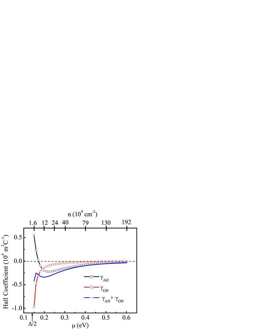
Figure 5: (Color online). The variation of anomalous Hall coefficient $\gamma_{AH}$, ordinary Hall coefficient $\gamma_{OH}$ and the total ($\gamma_{AH}$+$\gamma_{OH}$) with the chemical potential $\mu$. Here, $\rho_{xx}=10$ $k\Omega$, $\Delta=0.28$ $eV$, $t=2.82$ $eV$ and $a=2.46$Ȧ.

with $m_{e}$ being the bare electron mass. Figure 5 shows the comparison of the anomalous Hall coefficient with the ordinary one $\gamma_{OH}$ (=$-\frac{1}{ne}$) at zero temperature. It is shown that with increase of chemical potential, $\gamma_{AH}$ changes from positive to negative and has a curvature opposite to that of $\gamma_{OH}$. Moreover, we find that $\gamma_{AH}$ is comparable with $\gamma_{OH}$ for a typical value of $\rho_{xx}$=10 $k\Omega$[17] and becomes dominant for larger resistivity. It indicates that Hall coefficient may be detected as a signal of Berry curvature experimentally.

Valley-orbit coupling. The traditional theories of anomalous Hall effects are all based on two ingredients: spin polarization and spin-orbit coupling [18]. In our system, spin-orbit coupling is extremely weak [19], so we have ignored it from the very beginning. Because of the magnetic moment associated with the valleys, we are able to produce a population imbalance between the two valleys, i.e., a valley polarization, by a magnetic field. Is there a valley-orbit coupling that underlies the anomalous Hall effect discussed in this work?

From a phenomenological point of view, there is indeed a valley-orbit coupling, because electrons in two valleys do have opposite anomalous velocities under an electric field. In fact, the analogy with spin-orbit coupling can be made more precise if we consider the effective Hamiltonian for the conduction band. Ref.[13] has provided a recipe to construct the effective Hamiltonian from three basic ingredients: the band energy, the magnetic moment, and the Berry curvature. The magnetic moment gives rise to the Zeeman coupling between the magnetic field and the valley index. There is also a dipole-like term proportional to the electric field $e\textbf{E}\cdot\textbf{R}$, where $\bf R$ is the Berry connection potential defined by $\nabla_{k}\times\textbf{R}=\Omega$. Using the expression of the Berry curvature for the graphene system given by Eq.(2), we find that $\textbf{R}=-\frac{\tau_{z}}{2k^{2}}\left({1-\frac{\Delta}{{\sqrt{\Delta^{2}+3k^{2}a^{2}t^{2}}}}}\right)\textbf{k}\times\bf{\hat{z}}$. Therefore, the low-energy effective Hamiltonian [20] can be written as

$$H_{\text{eff}}=\varepsilon_{0}(\textbf{k})-\tau_{z}\mu^{*}_{B}\textbf{B}\cdot\hat{\textbf{z}}-\frac{\tau_{z}e\hbar^{2}}{4m_{e}^{*2}c^{*2}}\hat{\textbf{z}}\cdot(\textbf{k}\times\textbf{E}),$$ (7)

where $c^{*}=\frac{\sqrt{3}at}{2\hbar}$ is the electron speed at Dirac point of the gapless graphene. The third term is the valley-orbit coupling, which has the similar form as the spin-orbit coupling. The effective Hamiltonian resembles closely the Pauli Hamiltonian for free electrons in the non-relativistic limit.

In summary, we have studied the magnetic susceptibility and anomalous Hall effect in epitaxial graphene. Our results show that a large diamagnetism will result from the large valley magnetic moment of graphene electrons. We also predict an anomalous Hall coefficient, which can dominant that of the ordinary Hall effect, due to a valley dependent Berry phase or valley-orbit coupling.

Acknowledgments: The authors acknowledge useful discussions with D. Goldhaber-Gordon. This work is supported by NSF, DOE, the Welch Foundation, and CNSF.

[1]K. S. Novoselov et al., Nature 438, 197 (2005); Yuanbo Zhang et al., Nature 438, 201 (2005)
[2]A. K. Geim and K. S. Novoselov, Nat. Mater. 6, 183 (2007).
[3]Y. W. Son, M. L. Cohen and S. G. Louie, Phys. Rev. Lett. 97, 216803 (2006).
[4]S. Y. Zhou et al., Nat. Mater. 6, 770 (2007).
[5]A. Attausch and O. Pankratov, Phys. Rev. Lett. 99, 076802 (2007); F. Varchon et al., Phys. Rev. Lett. 99, 126805 (2007);J. Hass et al., Phys. Rev. Lett. 100, 125504 (2008).
[6]K. Novoselov, Nature Phys. 6, 720 (2007).
[7]T. Ando, Physica E 40, 213 (2007); J. W. McClure, Phys. Rev. 104, 666 (1956).
[8]G. W. Semenoff, Phys. Rev. Lett. 53, 2449 (1984).
[9]C. L. Kane and E. J. Mele, Phys. Rev. Lett. 95, 226801 (2005).
[10]We also calculated the magnetic susceptibility from tight binding model and find that the influence of valence band bottom on susceptibility can be neglected. When the chemical potential is in the gap, the susceptibility is calculated to be $-4.935\times 10^{-8}$ JT^-2m^-2, which is very close to our analytical result $-5.084\times$10^-8 JT^-2m^-2 ($\frac{{e^{2}a^{2}t^{2}}}{{4\pi\hbar^{2}\Delta}}$).
[11]Wang Yao, Di Xiao, and Q. Niu, Phys. Rev. B 77, 235406 (2008).
[12]Di Xiao, Wang Yao, and Q. Niu, Phys. Rev. Lett. 99, 236809 (2007).
[13]M.-C. Chang and Q. Niu, Phys. Rev. B 53, 7010 (1996).
[14]Di Xiao, Junren Shi and Q. Niu, Phys. Rev. Lett. 95, 137204 (2005).
[15]L Berger, Phys. Rev. B. 2, 4559 (1970).
[16]D. Culcer, A. H. MacDonald, and Q. Niu, Phys. Rev. B 68, 045327 (2003); J. Cumings et al., Phys. Rev. Lett. 96, 196404 (2006).
[17]$\rho_{xx}\sim 4k\Omega$ was observed in the gapless graphene[1]. However, in the staggered-potential graphene, back scattering process can not be prohibited completely, which leads to the large $\rho_{xx}$. Moreover, the substrate plays an important role on $\rho_{xx}$. For example, the resistivity of a bilayer graphene sample was 10⁵ $\Omega$ cm^-1 on a more insulating 4H-SiC substrate compared with 0.2 $\Omega$ cm^-1 in 6H-SiC[5].
[18]N. A. Sinitsyn, J. Phys:Condens. Matter20, 023201 (2008).
[19]H. Min et al., Phys. Rev. B 74, 165310 (2006); Y. Yao et al., Phys. Rev. B 75, 041401 (2007).
[20]M.-C. Chang and Q. Niu, J.Phys.:Condens. Matter 20, 193202 (2008).

FIG.1: (Color online). The Landau levels from exact quantum calculations for $\tau_{z}=+1$ (a) and $\tau_{z}=-1$ (b) valleys. For comparison, the energy dispersions $\varepsilon_{0}(\textbf{k})$ (dashed line) and $\varepsilon(\textbf{k})=\varepsilon_{0}(\textbf{k})-\textbf{m}(\textbf{k})\cdot\textbf{B}$ (solid curves) are shown. Parameters are $\Delta$= 0.28 $eV$, $t$= 2.82 $eV$ and lattice constant $a$=2.46 Ȧ.

FIG.2: (Color online). (a) Magnetic susceptibility as a function of chemical potential. (b) Magnetic susceptibility from conduction electrons only. Here, $T=$ 10 $K$ and $\Delta$= 0.28 $eV$.

FIG.3: (Color online). The field dependence of semiclassical Landau levels for $\tau_{z}=+1$ (red circle) and $\tau_{z}=-1$ (blue triangle) valleys. For comparison, the exact quantum Landau levels are also shown (solid line).

FIG.4: (Color online). (a)The variation of valley polarization $P_{V}$ with the magnetic field $B$ ($\mu$=0.2 eV). (b)The variation of valley polarization $P_{V}$ with the chemical potential $\mu$ (B=0.2 T). Both the quantum calculations (red) and semiclassical results (black) are shown.

FIG.5: (Color online). The variation of anomalous Hall coefficient $\gamma_{AH}$, ordinary Hall coefficient $\gamma_{OH}$ and the total ($\gamma_{AH}$+$\gamma_{OH}$) with the chemical potential $\mu$. Here, $\rho_{xx}=10$ $k\Omega$, $\Delta=0.28$ $eV$, $t=2.82$ $eV$ and $a=2.46$Ȧ.