Spectral functions for single- and multi-Impurity models using DMRG

Abstract

This article focuses on the calculation of spectral functions for single- and multi-impurity models using the density matrix renormalization group (DMRG). To calculate spectral functions in DMRG, the correction vector method is presently the most widely used approach. One, however, always obtains Lorentzian convoluted spectral functions, which in applications like the dynamical mean-field theory can lead to wrong results. In order to overcome this restriction, we use chain decompositions in which the resulting effective Hamiltonian can be diagonalized completely to calculate a discrete “peak” spectrum. We show that this peak spectrum is a very good approximation to a deconvolution of the correction vector spectral function. Calculating this deconvoluted spectrum directly from the DMRG basis set and operators is the most natural approach, because it uses only information from the system itself. Having calculated this excitation spectrum, one can use an arbitrary broadening to obtain a smooth spectral function, or directly analyze the excitations. As a nontrivial test we apply this method to obtain spectral functions for a model of three coupled Anderson impurities. Although, we are focusing in this article on impurity models, the proposed method for calculating the peak spectrum can be easily adapted to usual lattice models.

I Introduction

Impurity models can be considered as the most basic models for strongly correlated electron systems: a small region of interacting electrons coupled to a reservoir of electrons.Hewson (1997) The degrees of freedom on the impurity, the degrees of freedom in the reservoir, the coupling between the reservoir and the impurity, as well as the interactions on the impurity range very widely and depend on the physical situation of interest. These situations range from “real” impurities in metals, like cobalt in copper, artificial created nano-structures, to dynamical mean-field theory (DMFT). Besides their wide usage, also the physical effects inherent are very interesting. The most famous finding is the Kondo-effect Hewson (1997), which manifests itself as a narrow resonance in the single-particle spectrum of the Anderson impurity model.

To this day, there are many different methods for calculating properties of quantum impurity models: the numerical renormalization group (NRG)Wilson (1975); Bulla et al. (2008) and continuous-time quantum Monte CarloWerner et al. (2006); Gull et al. (2011) are two of the currently widely used. In this article we focus on the density matrix renormalization group (DMRG).White (1992); Schollwöck (2005, 2011) DMRG has proved to be a highly accurate method for calculating ground state properties of one-dimensional models. Thus, it is widely used for calculating expectation values and correlation functions of such chains gaining nearly numerical accuracy. DMRG has also already been used for calculating impurity propertiesNishimoto and Jeckelmann (2004); Raas et al. (2004); Raas and Uhrig (2005); Nishimoto et al. (2006) or as a DMFT-solverGarcia et al. (2004); Nishimoto et al. (2004); Karski et al. (2005, 2008); Raas et al. (2009).

A big advantage of DMRG and NRG is their ability to calculate spectral functions directly in the real frequency domain, making an ill-conditioned analytic continuation like in Quantum-Monte-Carlo unnecessary. In NRG and DMRG the Hamiltonian of the impurity model has to be mapped on a chain model, which is then diagonalized. As there are several similarities between both methods, we will compare the results of both, where it is possible.

In the next section of this article we introduce the Anderson impurity model, and we will compare the main features of DMRG and NRG. The third section is devoted to the calculation of spectral functions for the single impurity Anderson model. While ground state properties can be determined with very high precision using DMRG, spectral functions are much more difficult. We perform our calculations using the correction vector method,Kühner and White (1999); Jeckelmann (2002) resulting in a Lorentzian broadened spectral function. In the beginning of the third section we show that the inability of resolving sharp structures can give wrong results when being used in the self-consistency loop of the DMFT.Georges et al. (1996)

The main purpose of the first part of this article is to provide an extension of the existing correction vector method. We will show how a peak structure for the spectral function can be calculated by using complete diagonalization of an effective Hamiltonian. Having determined this peak structure an arbitrary broadening function can be used, increasing the resolution of the spectral function. Furthermore, we show that this peak structure is a very good approximation to a deconvolution of the correction vector spectral function.

Finally, in the last section we will go beyond the single impurity Anderson model, using the just introduced method for calculating spectral function for a three impurity model. For testing the newly developed extension of the correction vector method and the ability of DMRG to calculate spectral functions for multi-impurity systems, we couple three Anderson impurity models via a single-particle hopping. This will allow in future works to use DMRG as an impurity-solver in multi-orbital DMFT calculations or as a cluster-DMFT-solver.

II Single Impurity Anderson Model

We will start with the most simple impurity model, namely the single impurity Anderson model (SIAM).Hewson (1997) For deriving the Hamiltonian which can be solved via DMRG, we perform a discretization scheme similar to NRG.Bulla et al. (1997, 2008) Following the notation of Bulla et al. (2008), the Hamiltonian for the SIAM reads

$$H = \sum_{\sigma}\epsilon_{f}f_{\sigma}^{\dagger}f_{\sigma}+Uf_{\uparrow}^{\dagger}f_{\uparrow}f_{\downarrow}^{\dagger}f_{\downarrow}$$ (1)

$$+\sum_{k\sigma}\epsilon_{k}c_{k\sigma}^{\dagger}c_{k,\sigma}$$

$$+\sum_{k\sigma}V_{k}\left(f_{\sigma}^{\dagger}c_{k\sigma}+c_{k\sigma}^{\dagger}f_{\sigma}\right),$$

for which $f^{\dagger}_{\sigma}$ represents the impurity and $c_{k\sigma}^{\dagger}$ the band states. Herein, $U$ is the amplitude of a two-particle interaction on the impurity, $\epsilon_{f}$ the energy level of the impurity, and $\epsilon_{k}$ the energy dispersion of the conduction band electrons. Finally, $V_{k}$ represents the coupling between the impurity and the conduction band. The hybridization function, which completely describes the coupling between the impurity and the bath,Bulla et al. (1997) is given by

$$\Delta(\omega)=\pi\sum_{k}V_{k}^{2}\delta(\omega-\epsilon_{k}).$$

Assuming that the support of the hybridization is covered by the interval $[-1,1]$, we can rewrite the Hamiltonian as

$$H = \sum_{\sigma}\int_{-1}^{1}d\epsilon\;g(\epsilon)a_{\epsilon\sigma}^{\dagger}a_{\epsilon\sigma}$$ (2)

$$+\sum_{\sigma}\int_{-1}^{1}d\epsilon h(\epsilon)\left(f_{\sigma}^{\dagger}a_{\epsilon\sigma}+a_{\epsilon\sigma}^{\dagger}f_{\sigma}\right)$$

$$+\sum_{\sigma}\epsilon_{f}f_{\sigma}^{\dagger}f_{\sigma}+Uf_{\uparrow}^{\dagger}f_{\uparrow}f_{\downarrow}^{\dagger}f_{\downarrow},$$

for which $g(\epsilon)$ and $h(\epsilon)$ represent the dispersion and the coupling to the impurity, respectively. The relation between the hybridization function $\Delta(\omega)$, $g(\epsilon)$ and $h(\epsilon)$ is given by

$$\Delta(\omega)=\pi\frac{dg^{-1}(\omega)}{d\omega}h(g^{-1}(\omega))^{2}.$$

The Hamiltonian Eq. 2 can now be discretized by dividing $[-1,1]$ into disjunct intervals $I_{n}=[k_{n},l_{n}]$ with $\bigcup I_{n}=[-1,1]$. In NRG calculations, these intervals should be chosen as $k_{n}=\pm\Lambda^{-n}$, $l_{n}=\pm\Lambda^{-(n+1)}$ with $\Lambda>1$. However, in DMRG calculations these intervals can be freely chosen. As explained in detail in Bulla et al. (2008), one defines new fermionic operators for each of these intervals, so that the Hamiltonian finally becomes that of a one-dimensional chain, shown in Fig. 1, reading

$$H = \sum_{\sigma}\epsilon_{f}f_{\sigma}^{\dagger}f_{\sigma}+Uf_{\uparrow}^{\dagger}f_{\uparrow}f_{\downarrow}^{\dagger}f_{\downarrow}$$ (3)

$$+V\sum_{\sigma}\left(f_{\sigma}^{\dagger}c_{0\sigma}+c_{0\sigma}^{\dagger}f_{\sigma}\right)$$

$$+\sum_{n\sigma}\epsilon_{n}c_{n\sigma}^{\dagger}c_{n\sigma}$$

$$+\sum_{n\sigma}t_{n}\left(c_{n\sigma}^{\dagger}c_{n+1\sigma}+c_{n+1\sigma}^{\dagger}c_{n\sigma}\right).$$

Figure 1: (Color online) One-dimensional chain model for the SIAM.

II.1 NRG versus DMRG calculations

As we are going to give several NRG results for comparison, let us shortly describe the differences between NRG and DMRG. For detailed information about how these methods work, we refer to the reviews by Schollwöck (2011) (DMRG) and by Bulla et al. (2008) (NRG). Recently, there have also been several attempts to combine both methods.Saberi et al. (2008); Weichselbaum et al. (2009); Holzner et al. (2010); Pizorn and Verstraete (2011)

The main recipe for NRG is: Iteratively increase the length of the chain starting at the impurity site, diagonalize the Hamiltonian and truncate the high energy states, if the number of Fock space states exceeds a certain number $N$. This procedure can only work because the intervals during the discretization were logarithmically arranged leading to an exponentially decreasing coupling $t_{n}$ in the one-dimensional chain. Thus, having diagonalized the chain up to site $i$, one can assume that the remaining sites of the chain are only a small “perturbation”, as the coupling $t_{i}$ is small compared to the energy difference between the high energy states and the low energy states. Being only interested in the energetically low lying states, one can truncate the high energy states and treat them as approximate excited states of the whole chain, thus obtaining information about the whole spectrum of energies.

On the other hand, in DMRG one calculates from the beginning the ground state of the whole chain. DMRG combines left blocks and right blocks to calculate approximate ground states of the whole chain. The left and right blocks are gradually refined by calculating the “best” basis sets for those blocks, which best describe the ground state of the chain. This can be done by calculating the density matrix of the ground state for the blocks. Thus, DMRG is able to calculate very accurate ground states for one-dimensional chains, and does not necessarily need a logarithmic discretization of the conduction band.

One big difference between both methods is, that using NRG one can calculate a complete set of eigenstates of the model. Peters et al. (2006); Weichselbaum and von Delft (2007) This can only be achieved by the above described “energy separation” due to the logarithmic discretization. The disadvantage is that this logarithmic discretization reduces the resolution of high energy contributions, as they are worse resolved during the discretization. Furthermore, in NRG calculations one has to include always all states contributing to one “energy shell” (imposed by the discretization parameter $\Lambda$) for setting up the Hamiltonian up to site $i$. Going from the single impurity model to multi-impurities, having more than one conduction band, will lead to an exponential increase in matrix dimensions, eventually making calculations impossible or inaccurate with increasing number of conduction bands. On the other hand, in DMRG calculations one can easily separate each conduction band, as they only couple directly at the impurity to each other. Thus, only the impurity itself must be considered increasingly difficult within DMRG, as all conduction bands couple at this site. Additionally, in DMRG the discretization of the conduction band can be freely chosen, increasing the resolution of high energy contributions. These are clearly advantages of the DMRG. The price one pays is loosing the complete set of excited states calculated within NRG, because DMRG can only calculate properties of the ground state or a very few excited states.

III Spectral functions

III.1 Definition and Calculation

In this article we focus on the calculation of dynamical properties, such as Green’s functions. As Green’s functions depend on excited states, the calculation of these dynamical properties can be easily performed within NRG having a complete basis set. Within DMRG it is much more difficult, because the usual DMRG-basis set is optimized for the ground state, but excited states are not optimally represented.

Nevertheless, there are ways to calculate the Green’s function within DMRG. The definition of the fermionic one-particle Green’s function at $T=0$ corresponding to the ground state $|\Psi_{0}\rangle$, is given by

$$iG(t) := \Theta(t)\langle\Psi_{0}|[c(t),c^{\dagger}(0)]_{+}|\Psi_{0}\rangle$$

$$G(\omega) = \sum_{i}\left(\frac{\langle\Psi_{0}|c|\phi_{i}\rangle\langle\phi_{i}|c^{\dagger}|\Psi_{0}\rangle}{\omega+E_{0}-E_{i}+i\eta}\right.$$ (5)

$$+\left.\frac{\langle\Psi_{0}|c^{\dagger}|\phi_{i}\rangle\langle\phi_{i}|c|\Psi_{0}\rangle}{\omega-E_{0}+E_{i}+i\eta}\right)$$

$$= \Bigl{\langle}\Psi_{0}\Bigl{|}c\frac{1}{\omega+E_{0}-H+i\eta}c^{\dagger}\Bigr{|}\Psi_{0}\Bigr{\rangle}$$

$$+\Bigl{\langle}\Psi_{0}\Bigl{|}c^{\dagger}\frac{1}{\omega-E_{0}+H+i\eta}c\Bigr{|}\Psi_{0}\Bigr{\rangle},$$

with $\eta\rightarrow 0$, and $|\phi_{i}\rangle$ being a complete Fock space basis of eigenstates. Equation 5 is commonly called Lehmann representation and is used to calculate spectral function within NRG.Peters et al. (2006); Weichselbaum and von Delft (2007)

Unfortunately, such a complete basis set of eigenstates, $|\phi_{i}\rangle$, is usually not available within DMRG, as the emerging matrix sizes are too large for full diagonalization, so that iterative methods, such as Lanczos or Jacobi-Davidson, for calculating the ground state are used. However, as it is possible to calculate the result of an operator acting on a state, one can use Eq. 5 for calculating the Green’s function. The operator $\frac{1}{\omega+E_{0}-H+i\eta}$ acting on $c^{\dagger}|\Psi_{0}\rangle$ results in the so called correction vector,Kühner and White (1999); Jeckelmann (2002) from which a Lorentzian broadened spectral function can be calculated, corresponding to Eq. 5. The physical interesting spectral function would be obtained by taking the limit $\eta\rightarrow 0$. However, this limit $\eta\rightarrow 0$ cannot directly be performed, because the spectrum of a finite chain is discrete, giving a finite number of peaks at $\delta(\omega+E_{0}-E_{i})$. Therefore, one would have to know exactly $E_{i}$ and the corresponding eigenstate $|E_{i}\rangle$ (being equivalent to the knowledge of a complete basis set of eigenstates). Having no complete basis set of eigenstates, it is impossible to numerically calculate the operator $\frac{1}{\omega+E_{0}+i\eta-H}$ for $\eta\to 0$. Decreasing $\eta$ makes it more and more difficult to calculate a converged correction vector, increasing the necessary truncation dimension of the basis and the computation time.

Therefore, one has to use a finite $\eta>0$, resulting in a Lorentzian broadened spectral function. There are deconvolution schemesRaas and Uhrig (2005) like maximum entropy, calculating a Green’s function in the limit $\eta\rightarrow 0$ starting from the broadened correction vector spectral function, but their ability to resolve sharp features is rather limited. Furthermore, when using deconvolution schemes one usually has to allow for some small discrepancies between the convolution of the result and the DMRG spectral function. This introduces a new source of errors and arbitrariness into the final result. Other possibilities for calculating spectral functions within DMRG are expanding the spectral function into a continued fraction,Hallberg (1995); Dargel et al. (2011) expanding in Chebyshev polynomials,Holzner et al. (2011) or to use a Fourier transformation from a real-time calculation.Pereira et al. (2009) However, to this day the correction vector method is the most widely used method.

III.2 Problems within Dynamical Mean-Field Theory

Before showing a very natural way for obtaining a deconvoluted spectrum, we want to show the occurring problem when using DMRG in a DMFT self-consistency calculation. DMFT calculates a solution of a lattice model, like the Hubbard model, by mapping it onto a self-consistent impurity calculation.Georges et al. (1996) This self-consistency is usually obtained by iteratively solving the impurity model. Therefore, one has to deconvolute the result in every DMFT iteration, so that errors introduced by convolution/deconvolution can grow during the DMFT cycle.

Especially the frequencies around the Fermi energy are most important for the stabilization of a converged DMFT solution. The results can be entirely different depending on the existence of a gap at the Fermi energy.

Figure 2: (Color online) Comparison between spectral functions, $\rho(\omega)=-\mathfrak{Im}(G(\omega))/\pi$, of DMFT calculations for the antiferromagnetic Néel state in the Hubbard model (Bethe lattice, $U=W$, $T=0$, different chemical potentials $\mu$) using DMRG and NRG as impurity solver. The left panels are calculated via DMRG, the right panels via NRG. Blue and orange lines correspond to spin-up and spin-down, respectively. For the DMRG correction vector we used $\eta=0.25W$.

An example for this is given in Fig. 2. The figure shows DMFT results for the antiferromagnetic state in the Hubbard model,

$$H=t\sum_{\langle i,j\rangle,\sigma}c_{i\sigma}^{\dagger}c_{j\sigma}+U\sum_{i}n_{i\uparrow}n_{i\downarrow},$$

for $U=W$, $U$ being the local interaction strength and $W=4t$ the bandwidth of the non-interacting electron system for a Bethe lattice. The results as given by NRG show a phase separation between the antiferromagnetic phase at half filling and the paramagnetic state away from half filling.Peters and Pruschke (2009) The shown DMRG results are deconvoluted by a non-biased Maximum Entropy scheme.Raas and Uhrig (2005) Non-biased means that we have not used any additional assumptions for the result of the spectral function. For the DMRG correction vector, a broadening of $\eta=0.25W$ has been used. This example is somewhat extreme using a very large broadening. However, as all structures in the spectral function must be included into the discretization interval $[-1,1]$, such situations can occur, as the position of structures depend not only on the bandwidth $W$, but also on the interaction strength and the chemical potential. In this specific chosen example the features in the original convoluted spectral function as calculated by DMRG are smeared out. Deconvolution is able to sharpen the contours, but it cannot resolve detailed structure.

The half filled solutions of DMRG and NRG in Fig 2 look quite similar. The main difference is that there is no real gap at the Fermi energy, $\omega=0$, in the DMRG result. The situation is worse for $\mu=-0.3W$, corresponding to a non-particle-hole-symmetric situation. The NRG/DMFT result is still an antiferromagnetic half filled Néel state, $\langle n_{\uparrow}+n_{\downarrow}\rangle=1$. This state is still gapped at the Fermi-energy, but the lower Hubbard band has moved towards the Fermi-energy. DMRG cannot resolve this very sharp structure near the Fermi-energy, and entirely closes the gap during the self-consistency cycle, even though deconvolution has been used. Thus, it appears, as if the DOS for the spin-up and spin-down components are just shifted apart from each other, resulting in a doped antiferromagnetic metallic state. We want to emphasize, that this DMRG/DMFT result is not just a differently broadened version of the NRG/DMFT result, but is a different solution due to the self-consistency. Only again for larger doping NRG and DMRG show both a paramagnetic metallic state, which reasonably agree with each other.

III.3 Calculating the peak spectrum

In general it is impossible to obtain a complete basis of eigenstates for the whole chain, because the Fock space dimension is too large. However, DMRG automatically creates basis sets for parts of the chain best describing the aimed states, e.g. the ground state. From these basis sets an effective Hamiltonian is set up and diagonalized. Usually working with high truncation dimensions to obtain an accurate result, the resulting dimensions for the effective Hamiltonian are still too large for complete diagonalization. (By “complete diagonalization” we mean, that all eigenstates and eigenvalues are calculated.) Nevertheless, there are several possibilities to obtain an effective description of the chain consisting of a Fock space dimension, which is small enough for complete diagonalization: e.g. left and right block can be strongly truncated and combined without a single block in between, or at the open boundaries of the chain, at which the basis dimension is in general smaller due to the boundary, see Fig. 3.

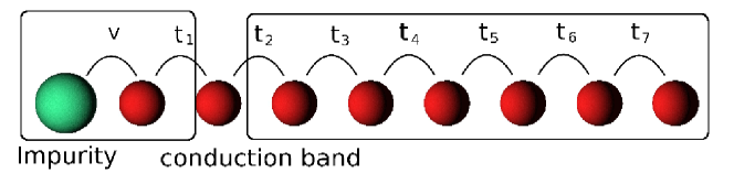
Figure 3: (Color online) DMRG chain with impurity, showing a position at which the effective Fock space dimension is reduced due to the open boundary.

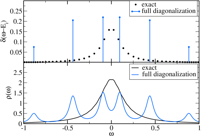
Figure 4: (Color online) Impurity spectral functions calculated by a complete diagonalization of an effective Hamiltonian. The chain decomposition consists of two local sites on the left side and a truncated “right-block” (linear discretization of the conduction electrons, $U=0$, $\Delta=0.1$, DMRG-truncation $m=300$). Upper panel: spectral weights from DMRG compared to the exact result calculated by diagonalization of the non-interacting hopping chain. Lower panel: Lorentzian broadening of the spectral weights using $\eta=0.05$.

Having a small effective basis set describing the whole chain, one can completely diagonalize the effective Hamiltonian and calculate the discrete peaks of the spectral function.

Figure 4 shows the resulting peaks in the spectral function, $\rho(\omega)=-\mathfrak{Im}(G(\omega))/\pi$, and a Lorentzian broadening of these peaks for the non-interacting SIAM, $U=0$, compared to the exact result calculated from the discretized one-particle Hamiltonian. First of all, it should be clear that the number of calculated peaks is small, and the position and weight of the peaks do not agree with the exact result. Although there are only $6$ peaks visible, the used Fock space basis consists of approximately $100$ states at this point. However, most of the excited states have zero weight in the spectral function. Thus, this straightforward implementation of calculating the spectral function by a complete diagonalization of an effective Hamiltonian yields not enough contributing states and fails. This corresponds to the optimization of the basis towards the ground state of the system. What is needed, is a change in the basis set towards excited states contributing to the spectral weight. This optimization of the DMRG basis can be achieved by the already introduced correction vector Kühner and White (1999); Jeckelmann (2002)

$$\frac{1}{\Omega+E_{0}-H+i\eta}c^{\dagger}|\Psi_{0}\rangle$$

$$= \sum_{i}|E_{i}\rangle\langle E_{i}\Bigl{|}\frac{1}{\Omega+E_{0}-E_{i}+i\eta}c^{\dagger}\Bigr{|}\Psi_{0}\rangle.$$

We label the frequency at which the correction vector is calculated as $\Omega$. Obviously, excited states, for which $\Omega+E_{0}\approx E_{i}$ holds, have strong weight in the correction vector. Thus, trying to optimize the ground state and the correction vector will optimize the basis towards contributing states. Of course, this is not surprising, as the correction vector exactly describes the spectral function.Kühner and White (1999); Jeckelmann (2002) However, instead of calculating only the value of the spectral function at $\Omega$, we now completely diagonalize the set up Hamiltonian, which yields the possibility to directly observe the contributing excited states $|E_{i}\rangle$. A similar idea has already been used in Kühner and White (1999), in which the correction vector was used for adapting the DMRG basis set followed by the calculation of the spectral function via the Lanczos method.

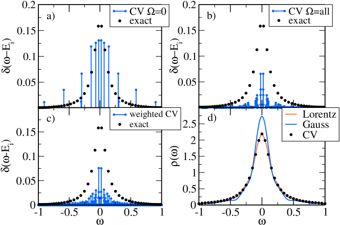
Figure 5: (Color online) Spectral weights calculated by diagonalization including the correction vector for the non-interacting SIAM $U=0$, $\Delta=0.1$. The conduction electrons were discretized linearly using $N=50$ sites. The correction vector used $\eta=0.05$. a) spectral weights of the correction vector (CV) for $\Omega=0$ compared to the exact results. (Chain decomposition as in Fig. 4) b) spectral weights of correction vectors $\Omega=\{-1.55,1.5,...,1.5,1.55\}$. c) spectral weights of the correction vectors weighted according to their position. d) Lorentzian ($\eta=0.05$) and Gaussian ($b=0.045$) broadened spectral functions compared to data points of the correction vector.

Figure 6: (Color online) Spectral function for the SIAM ($\Delta=0.1$, linear discretization $N=50$ sites, Chain decomposition as in Fig. 4) for different interaction strengths $U$ (upper panel: $U=0.4$ (left); $U=0.8$ (right). lower panel: $U=1.2$ (left); $U=2.0$ (right). We compare between the usual correction vector (CV) result $\eta=0.05$, a Gaussian broadening ($b=0.045$) of the calculated peaks, a Lorentzian broadening using $\eta=0.05$, and the NRG-result. The left inset in each panel gives the calculated level structure. The right inset in the lower panels gives a magnification around the Fermi energy.

Figure 5 shows again the calculated spectral weights using correction vectors, $\eta=0.05$, for the non-interacting SIAM, $U=0$, and $\Delta=0.1$. For comparison the exact peaks are included again. It should be stated that one cannot expect that DMRG calculates the exact positions of these peaks, as DMRG works in a restricted basis setting up an effective Hamiltonian. However, it is important that the summed up spectral weight around a frequency is approximately the same as in the exact result. Panel a) shows the spectral weight using only the correction vector at $\Omega=0$. Comparing to Fig. 4, the weight is now distributed over more states, especially near $\omega=0$. But for $|\omega|>0.2$ there are only a very few contributing states. Panel b) shows the spectral weights as a sum of all used correction vectors, $\Omega=\{-1.55,1.5,...,1.5,1.55\}$. For each frequency $\Omega$ a separate correction vector calculation followed by a complete diagonalization of the effective Hamiltonian is performed. As the final spectral function should be normalized, the weight of the peaks is divided by the number of used correction vectors. Again, the spectrum shows regions having only very small spectral weight, e.g. $\omega\approx 0.15$, although the exact result shows weight in those regions. The main reason for this behavior is the renormalization. If only a few correction vectors are contributing in those regions, the weight is renormalized, when dividing by the number of used correction vectors. One can easily overcome this problem by taking into account the position of the correction vectors, $\Omega$, as the spectral weights are supposed to be most accurate around this frequency. Thus, we can assign a weight to the spectral peaks using a Lorentzian function having the same $\eta$. Denoting a peak at $E_{i}$ calculated by the correction vector $\Omega$ as $p_{i}(E_{i},\Omega)$, we transform all peaks to

$$P_{i}(E_{i},\Omega)=\frac{1}{Z}\frac{\eta}{\pi}\frac{1}{(\Omega-E_{i})^{2}+\eta^{2}}\;p_{i}(E_{i},\Omega),$$

in which $Z$ is a constant factor normalizing the sum of the spectral weight to unity. The result of this transformation can be seen in panel c) of Fig. 5. The distribution of the spectral weights follows now the exact result. Finally these peaks can be broadened using an arbitrary broadening-functions. Panel d) shows the result using a Gaussian and a Lorentzian broadening. For the Lorentzian broadening we use the same $\eta$ as for the correction vector. For the Gaussian broadening we use $\delta(\omega-E)\to\frac{1}{b\sqrt{\pi}}\exp\left(-(\omega-E)^{2}/b^{2}\right)$. The result of this Lorentzian broadening is in very good agreement with the correction vector points. We want to stress this point, as it means that the calculated peak structure represents a deconvolution of the correction vector spectral function. This deconvolution is calculated directly within the DMRG basis. No additional methods or assumptions have to be used. Using a Lorentzian broadening upon the exact spectral poles, calculated from the one-particle Hamiltonian, agrees with this calculated curve. Unfortunately, it is not the general case that the Lorentzian broadening of the calculated peaks yields exactly the same result as the correction vector spectral function. Usually, there will be small derivations, due to the changing of the basis set for every correction vector. Nevertheless, the calculated peak structure gives a very good approximation to a full deconvolution of the correction vector result, which can be seen in the next examples.

Figure 6 shows several results for the interacting SIAM for $\Delta=0.1$. The interaction strengths range from $U=0.4$ to $U=2.0$. We chose a linear discretization of the conduction band with $N=50$ sites for the DMRG calculation and compare between the usual correction vector (CV) result, NRG, and a broadening of the calculated peak structure. For $U=0.4$ ($U/\Delta=4$), there is still a broad and Lorentzian like peak at $\omega=0$. For this interaction strength, all curves reasonably agree with each other, taking into account that different broadening functions were used. Increasing the interaction strength, one can observe how the typical three-peak structure in the SIAM evolves. These three peaks can also be nicely observed in the calculated peak structure itself. Even for $U=2$, for which the Kondo resonance is hardly visible in the broadened DMRG results, one can still observe a peak near $\omega=0$ in the peak structure. Obviously, NRG can resolve the Kondo resonance for those interaction values, but fails to precisely resolve the Hubbard bands. Nevertheless, using a discretization parameter $\Lambda=2$ and a logarithmic-Gaussian broadening ($b=0.8$),Bulla et al. (2008) also NRG fails to precisely obtain $\rho(0)=1/(\Delta\pi)=3.183$. Although there are ways to improve this result (z-averaging or directly calculating the self-energy)Bulla et al. (2008), these techniques were not used here to present a comparison to a “basic” NRG-calculation. DMRG results show a homogeneous resolution for the whole spectral function. The Lorentzian broadening of the calculated peaks, agrees in all four examples very well to the correction vector points. Again, this is equivalent to the statement that the calculated peak structure corresponds to a deconvolution of the correction vector spectral function.

The spectral functions in Fig. 6 calculated by broadening of the peaks, show some oscillations, especially in the Hubbard peaks. These oscillations are stronger pronounced in the Gaussian broadened spectral functions, because the Lorentzian broadening smooths those oscillations. The shape of those structures depend on the number of used correction-vectors, the number of states kept during the DMRG-sweep and the exact decomposition of the chain to create the effective Hamiltonian.

Figure 7: (Color online) Spectral function for the SIAM ($\Delta=0.1$, $U=0.8$, linear discretization $N=50$ sites). Left: Lorentzian broadening. Right: Gaussian broadening ($b=0.045$). A two-block decomposition is used for calculating the peak structure. “Site” corresponds to the rightmost site in the left block. The impurity is located at site 0. The insets show a magnification of the Hubbard peak.

Figure 7 shows the calculated spectral function created by different chain decompositions for $U/\Delta=8$. For all shown spectral functions a two-block decomposition was used, for which the label “site” corresponds to the rightmost site in the left block. To obtain an effective basis which can be completely diagonalized the blocks are additionally truncated to $100$ states. This figure illustrates the dependence of the oscillations on the decomposition of the chain. However, this figure also shows that the proposed algorithm is not limited to decompositions near the open boundary at which the impurity is located. When the spectral functions is calculated in a decomposition, in which the impurity is located in a truncated block, the spectral weight does not have to sum up to unity. However, when the correction vector is included into the density matrix as target state, the spectral weight is reduced in the shown examples by approximately $10\%$, keeping $m=300$ states during the calculation. The spectral weight was normalized to unity in Fig. 7. The oscillations are naturally more pronounced in the Gaussian broadening, as this broadening is used here to enhance the resolution of small structures.

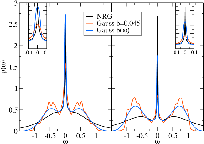
Figure 8: (Color online) Spectral functions for the SIAM ($\Delta=0.1$, $N=50$ sites) using different broadening schemes. Left panel: $U=0.8$ Right panel: $U=1.2$. The insets show a magnification around the Fermi energy.

One very big advantage having calculated the peak structure is obviously that one can immediately change the broadening of the peaks. To resolve the Kondo resonance at $\omega=0$ without introducing too many oscillations for $|\omega|>0$ one can now use a frequency dependent broadening focusing on the Kondo resonance. In Fig. 8 we compare the NRG result to an usual Gaussian broadened spectral functions and a frequency-dependent broadening, in which the position of the peak determines the broadening parameter as $b(E_{i}):=|1.5E_{i}|$. This allows for sharp structures at $\omega\approx 0$, but smoothing oscillations for large $\omega$. The shown results are for $U=0.8$ (left panel) and $U=1.2$ (right panel). Especially for $U=0.8$, the frequency dependent broadening resolves well the Kondo resonance and the Hubbard bands. The calculated shape of the Kondo-resonance, of course, depends on the used broadening. As NRG uses a Gaussian-logarithmic broadening,Bulla et al. (2008) the shape differs from the DMRG result. Whereas the NRG result determines a smaller width of the Kondo-resonance for $U=1.2$, the width of the DMRG result stays nearly unchanged. To understand this, it is advisable to directly analyze the calculated peak structure.

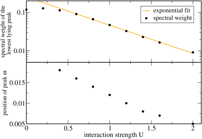
Figure 9: (Color online) Analysis of the lowest lying excitation for the SIAM $\Delta=0.1$ and $N=50$ sites for different interaction strengths. Upper panel: weight of the lowest lying peaks on logarithmic scale. Lower panel: position of the lowest lying peak.

In Fig. 9 we analyze the energetically lowest peaks in the spectral function of the SIAM as seen by the DMRG. The upper and the lower panel give the weight and the position of the peak, respectively. For the interaction values under consideration the spectral weight begins to exponentially decrease, which is the expected behavior for Kondo-physics. Also the position of the peak moves closer to $\omega=0$ when increasing the interaction strength. As this peak is supposed to describe the Kondo-resonance, its position is supposed to exponentially approach $\omega=0$ with increasing interaction strength. However, this is clearly not the case. The expected Kondo temperature for $U=2.0$ and $\Delta=0.1$ is approximately $T_{K}\approx 10^{-4}$, but the lowest lying peak is located at $\omega\approx 0.005$. This is because the chain has been discretized linearly with $N=50$ sites, setting an energy scale of $\Delta E=0.04$, as the conduction band electrons have energy from $-1$ to $1$. Structures below this value are hard to resolve. Unfortunately, increasing the number of sites or changing the discretization helps only to a limited amount. The resolution is also limited by the number of Fock space states, for which the complete diagonalization is performed, by the truncation of the DMRG basis set, and the used $\eta$ in the correction vector. We also performed calculations using a logarithmic discretization of the conduction band. The result is that for example the position of the lowest peak moves for $U=1.2$ from $\omega\approx 0.01$ to $\omega\approx 0.007$, thus giving only a little improvement for the Kondo resonance compared to the linear discretization. However, the high energy features of the spectral function turned out to be much more oscillating. The best results for spectral functions were obtained by using a linear discretization mesh corresponding to $\eta$ in the correction vector. Thus, though we can increase the resolution by calculating the peak structure, the resolution of the spectral function remains limited due to truncation and discretization of the chain.

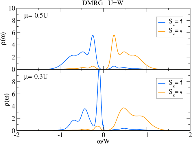
Figure 10: (Color online) DMFT calculations (Bethe lattice, $U=W$) using DMRG as impurity solver. The spectral functions are calculated using a Gaussian broadening upon the calculated peak spectrum with broadening $b=0.045$.

Finally, let us come back to the problem of convolution/deconvolution within DMFT calculations. Figure 10 shows again results for the antiferromagnetic phase in the Hubbard model for $U=W$ (compare to Fig. 2). This time the spectral functions were calculated using the above described method for determining the peak spectrum and later convoluted using a Gaussian broadening to obtain smooth curves. These results agree now very well with the known results from NRG. Both solution correspond to half filling showing a gap at the Fermi energy. Thus, we were able to improve the resolution of the spectral functions using the above described method.

Let us shortly summarize this section. We have shown that one can gain easily additional information about the spectral function while doing a correction vector calculation. These information are obtained by a complete diagonalization of the effective Hamiltonian created by the DMRG-basis including the correction vector. This is possible because the Fock space is small close to the open boundary, where the impurity is located. As this complete diagonalization is only performed, when a converged DMRG basis set for a correction vector is found, the additionally used time is negligible. Changing the correction vector, also changes the DMRG basis, finally giving a dense spectrum of peaks. This peak structure approximates a full deconvolution of the correction vector spectral function, in the sense that a Lorentzian broadening of these peaks results nearly in the correction vector spectral function. Besides representing a deconvolution, one can analyze those peaks directly or use an arbitrary broadening function.

IV Going Beyond Single Impurity Calculations

Besides being able to calculate spectral functions of the single impurity Anderson model with homogeneous resolution, DMRG is also able to perform calculations for multi-impurity systems, for which the model consists of more than one conduction channel and possibly more than one interacting sites. In NRG calculations, one has to combine all degrees of freedom for one energy shell to one single site. This results in an exponentially growing local Fock space when increasing the number of conduction bands. Therefore, NRG is currently limited to a very few conduction bands. As different conduction bands only couple directly at the impurity, it is easy to split these bands in a DMRG calculation. It is even possible to split the spin-up and spin-down electron degrees of freedom of the conduction bands, as also they only couple at the impurity.

For testing the abilities of DMRG to calculate spectral functions for multi-impurity models, we have performed calculations for a three-site impurity model, as visualized in Fig. 11.

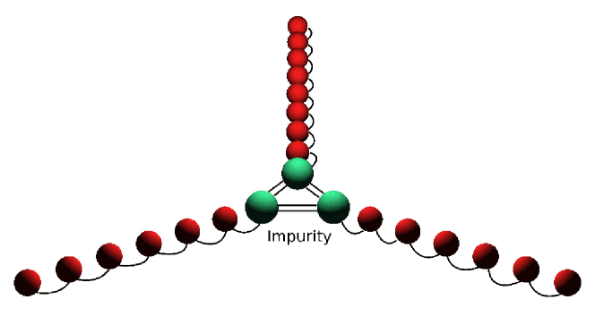
Figure 11: (Color online) Structure of the discretized three-site impurity model. The impurity sites (green) are the only sites including a two-particle interaction, coupling different conduction bands. As in the SIAM, the conduction bands are non-interacting sites with nearest neighbor hopping.

We include only an intra-band density-density interaction $U$ on the impurity site and a hopping $t^{\prime}$, coupling different impurity sites. The Hamiltonian thus reads

$$H = H_{Imp}+H_{cond}$$ (6)

$$H_{Imp} = \epsilon_{f}\sum_{l\sigma}f_{l\sigma}^{\dagger}f_{l\sigma}+U\sum_{l}f_{l\uparrow}^{\dagger}f_{l\uparrow}f_{l\downarrow}^{\dagger}f_{l\downarrow}$$

$$+t^{\prime}\sum_{l\neq n\sigma}f_{l\sigma}^{\dagger}f_{n\sigma}$$

$$H_{cond} = V\sum_{l\sigma}\left(f_{\sigma}^{\dagger}c_{l0\sigma}+c_{l0\sigma}^{\dagger}f_{l\sigma}\right)$$

$$+\sum_{li\sigma}t_{i}\left(c_{li\sigma}^{\dagger}c_{li\sigma}+c_{li\sigma}^{\dagger}c_{li\sigma}\right),$$

in which $l$, $n$ are channel indices, running from $1$ to $3$, $i$ is the site-index in a conduction band, and $\sigma$ the spin-index. The shown impurity Hamiltonian is just an example. In principle it is no problem to include other types of interactions on the impurity.

We start the DMRG calculation in one of the conduction electron chains including only the corresponding impurity site, firstly neglecting the other two chains. Having initialized this chain, all matrices are copied to the other chains. Thus, all three chains are described by the same basis set, just changing the band index. Copying the basis sets will prevent breaking the symmetries between the chains during the initialization, but is only justified in the case in which all conduction bands are supposed to be equal. The next DMRG step is the most time-consuming step. All three chains, which are described by $m$ states, have to be coupled as a Y-junction.Guo and White (2006) Thus, the dimension of the Fock space is now $m^{3}$. The diagonalization of the Hamiltonian is not the only time-consuming part, also the diagonalization of the density matrix, becomes very time-consuming, as it has dimension $m^{2}$ and must be diagonalized completely. After combining two conduction bands, there is one block describing the basis of two chains. Having calculated this “two-chain” block, DMRG works in the usual way improving the basis set of the remaining chain, always calculating the ground state for the whole system. To accelerate the convergence we always copy the improved basis set to the other two chains.

To calculate the peak structure as described in the previous section, we now have to use a two-block configuration, because the impurity is not located at an open boundary anymore. The used configuration consists of a left-block, describing two chains, and a right-block, describing the other chain. For the purpose of complete diagonalization for calculating the spectral function, the blocks are additionally truncated to $100$ states. Results for the non-interacting case are given in Fig. 12.

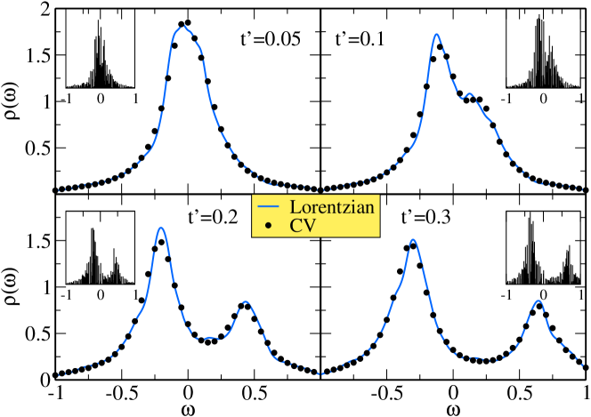
Figure 12: (Color online) Spectral function for a non-interacting three-Impurity Anderson Model, $\Delta=0.1$, $U=0$, $\epsilon_{f}=0$. The impurities are coupled by a hopping $t^{\prime}=\{0.05,0.1,0.2,0.3\}$ to each other. We compare the direct correction vector result (CV), $\eta=0.05$, to the Lorentzian broadening of the calculated peak structure. The DMRG used $m=300$ kept states.

For all the shown multi-impurity calculations we use a linear discretization consisting of 50 sites for each channel. We compare the calculated correction vector result, the calculated peak structure, and a Lorentzian broadening of the peaks for four different hopping amplitudes between the impurities. Calculating the exact result for this hopping Hamiltonian and using the same Lorentzian-broadening as in the correction vector, agrees with the calculated correction vector points. The physics can already be understood by coupling only three sites to a triangle by a hopping $t^{\prime}$. This three-site Hamiltonian has two single-particle-excitation, namely at $-t^{\prime}$ and $2t^{\prime}$. Coupling a conduction band to each of the impurities, results in a broadening of each of those excitations. Furthermore, by coupling three sites to a triangle, the particle-hole-symmetry is immediately broken.

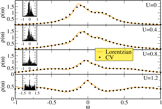
Figure 13: (Color online) Spectral function for a three-Impurity Anderson Model, $\Delta=0.1$. The impurities are coupled by a hopping $t^{\prime}=0.1$ to each other. The panels show different interaction strengths $U=(0.0;0.4;0.8;1.2)$ ($\epsilon_{f}=-U/2$) on the impurity sites. We show the calculated correction vector result (CV) and the Lorentzian broadening of the peak structure, which can be seen in the inset. The DMRG used $m=300$ kept states.

Figure 13 shows the results for the interacting case with $\Delta=0.1$. The hopping between the impurities is chosen as $t^{\prime}=0.1$, resulting in peaks at $\omega=-0.1$ and $\omega=0.2$ for the non-interacting model. Switching on the interaction, one can observe, how an asymmetric Kondo-resonance appears by merging of the two non-interacting peaks. Comparing between the correction vector points and the Lorentzian broadening of the calculated peak structure, we find again good agreement. So even in this difficult model, for which the impurity is not located anymore at the boundary, we are able to calculate a reliable peak structure.

An interaction or hopping between different impurities introduces entanglement between the chains. Combining the chains to a single block is therefore the step, at which the truncated weight can be very high, as the dimension is reduced from $m^{2}$ to $m$.

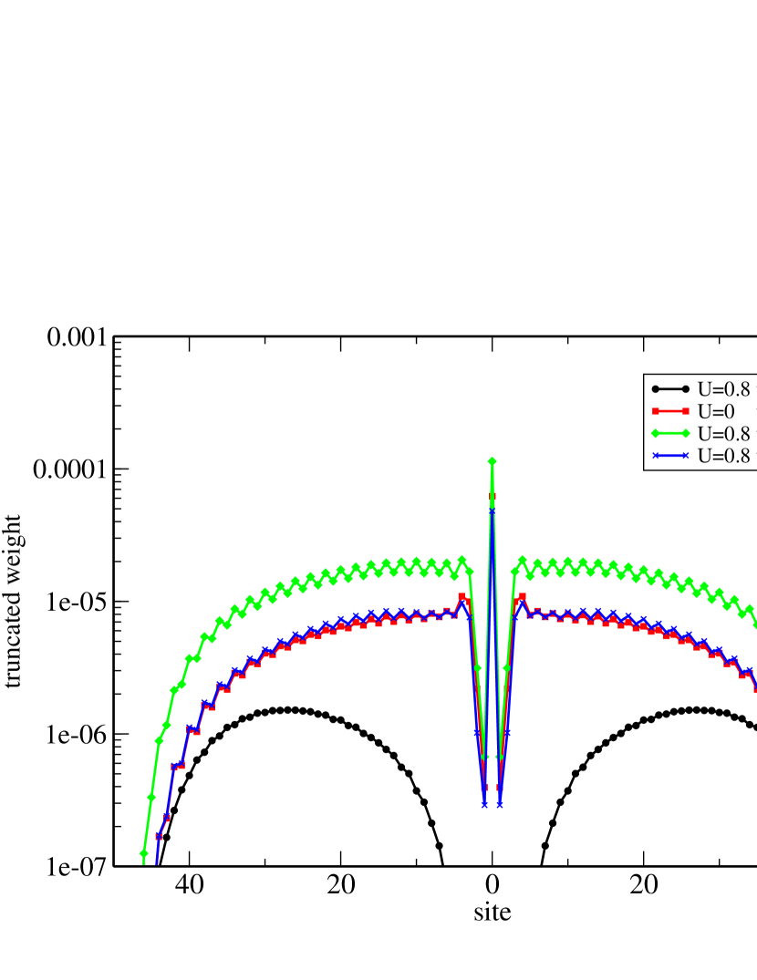
Figure 14: (Color online) Truncated weight for a ground state calculation of the three-impurity system ($\Delta=0.1$, $\epsilon_{f}=-U/2$). As reference a calculation without coupling between the impurities is shown ($t^{\prime}=0$). The label “site” corresponds to the middle block of the used three-block DMRG algorithm. “site=0” represents the point at which two chains are combined to one block. (Further explanation in text.)

Figure 14 shows three examples for the truncated weight for such three-impurity calculations. For comparison the truncated weight for a calculation without coupling between the impurities is shown, too. The index “site=0” represents the point at which two chains are combined to one block. Without any coupling between the impurities, the ground state can be written as product state of three single-impurity models, for which the impurity is located at an open boundary. Therefore, the truncated weight vanishes at “site=0” in this case. When the impurities are coupled, combining two chains to one block produces a significant peak in the truncated weight. Keeping $m=200$ states, the truncated weight when combining the chains, is approximately $\delta\rho\approx 10^{-4}$. Increasing the kept states to $m=300$, decreases the truncated weight to $\delta\rho\approx 5\cdot 10^{-5}$. Keeping $m=300$ states in the shown examples, the ground state energy as well as impurity expectation values like occupation do not change in their first 5 digits during DMRG sweeping after convergence is achieved. When calculating the spectral function and thus including the correction vector into the density matrix, the truncated weight is increased. However, the calculated spectral functions for the non-interacting case ($U=0$) agree very well with the exact spectral functions, as already mentioned above.

It is in principal easy to go even beyond three conduction bands. Increasing the number of conduction bands will eventually make it impossible to couple all bands at the same DMRG step. However, it is always possible to iteratively couple the different conduction bands, which, of course, will even increase the truncation error. Nevertheless, we have demonstrated that it is possible to calculate multi-impurity properties using DMRG, making it possible to use DMRG in multi-orbital DMFT or cluster-DMFT calculations.

V Conclusions

We have used the DMRG to calculate spectral functions for single and multi-impurity models. We discretized the conduction band electrons using the same scheme as in NRG. However, using DMRG gives more freedom of choosing the intervals for the discretization, because DMRG does not rely on energy separation. Therefore, the hopping parameters in the discretized conduction electron chain can be arbitrary, and orbital and spin degrees of freedom of the conduction electrons can be split. A disadvantage of DMRG arises when calculating spectral functions, as the DMRG basis is very optimized for the ground state. Nevertheless, there are different methods to calculate spectral functions within DMRG, but usually the resolution is limited. This limitation can lead to unphysical solutions when using DMRG as an impurity solver in DMFT.

We here used the correction vector method, from which a Lorentzian convoluted spectral function can be calculated. To improve the resolution, we used a complete diagonalization of the DMRG basis in special configurations and calculated a peak structure of the spectral function. It is essential to adapt the DMRG basis via the correction vector so that also excitation are well described. By performing these diagonalization for different correction vectors, a dense set of peaks can be calculated. It should be noted that the additional time cost is negligible to the rest of the correction vector calculation. This peak structure can be directly analyzed as for example extracting the weight and position of sharp features. It also helps understanding what structures can actually be resolved, as it exactly shows the basis from which the correction vector spectral function is calculated. Besides this, these peaks can be convoluted using an arbitrary broadening function creating a smooth spectral function. Thus, it is easy to change the convolution from Lorentzian (correction vector) to any other function. Finally, this peak structure represents a very good approximation to a deconvolution of the correction vector spectral function.

In the second part of this article, we used this technique for a model, in which three Anderson impurity models are coupled via a hopping. We show, that it is again possible to use the introduced algorithm to obtain a peak structure of the spectral function. We thus are able to calculate precise spectral function for this model, making future application of DMRG as Cluster-DMFT solver possible.