Formation rates of dark matter haloes

Abstract

We derive an estimate of the rate of formation of dark matter haloes per unit volume as a function of the halo mass and redshift of formation. Analytical estimates of the number density of dark matter haloes are useful in modeling several cosmological phenomena. We use the excursion set formalism for computing the formation rate of dark matter haloes. We use an approach that allows us to differentiate between major and minor mergers, as this is a pertinent issue for semi-analytic models of galaxy formation. We compute the formation rate for the Press-Schechter and the Sheth-Tormen mass function. We show that the formation rate computed in this manner is positive at all scales. We comment on the Sasaki formalism where negative halo formation rates are obtained. Our estimates compare very well with N-body simulations for a variety of models. We also discuss the halo survival probability and the formation redshift distributions using our method.

1 Introduction

Gravitational amplification of density perturbations is thought to be responsible for formation of large scale structures in the Universe (Peebles, 1980; Shandarin & Zeldovich, 1989; Peacock, 1999; Padmanabhan, 2002; Bernardeau et al., 2002). Much of the matter is the so called dark matter that is believed to be weakly interacting and non-relativistic (Trimble, 1987; Komatsu et al., 2009). Dark matter responds mainly to gravitational forces, and by virtue of a larger density than baryonic matter, assembly of matter into haloes and large scale structure is primarily driven by gravitational instability of initial perturbations in dark matter. Galaxies are believed to form when gas in highly over-dense haloes cools and collapses to form stars in significant numbers (Hoyle, 1953; Rees & Ostriker, 1977; Silk, 1977; Binney, 1977). Thus the hierarchical formation of dark matter haloes is the key driver that leads to formation and evolution of galaxies and clusters of galaxies.

The halo mass function describes the comoving number density of dark matter haloes as a function of mass and redshift in a given cosmology. It is possible to develop the theory of mass functions in a manner that makes no reference to the details of the cosmological model or the power spectrum of fluctuations. That is, we expect the mass function to take a universal form, when scaled appropriately. Simple theoretical arguments have been used to obtain this universal functional form of the mass function (Press & Schechter, 1974; Bond et al., 1991; Sheth, Mo, & Tormen, 2001). Bond et al. (1991), and, Sheth, Mo, & Tormen (2001) used the excursion set theory to derive the mass function. Much work has also been done to determine the extent to which this form is consistent with results from N-body simulations (Jenkins et al., 2001; White, 2002; Reed et al., 2003; Warren et al., 2006; Reed et al., 2007; Lukić et al., 2007; Cohn & White, 2008; Tinker et al., 2008) with the conclusion that the agreement is fairly good. It is remarkable that a purely local approach provides a fairly accurate description of the manifestly non-linear and strongly coupled process of gravitational clustering. The success of the local description has been exploited in developing the semi-analytic theories of galaxy formation (White & Frenk, 1991; Kauffmann, White & Guiderdoni, 1993; Chiu & Ostriker, 2000; Madau, Ferrara, & Rees, 2001; Samui et al., 2007).

The Press-Schechter mass function (Press & Schechter, 1974) that is commonly used in these semi-analytic models assumes spherical collapse of haloes (Gunn & Gott, 1972). The shape of this mass function agrees with numerical results qualitatively, but there are deviations at a quantitative level (Efstathiou et al., 1988; Jenkins et al., 2001). Improvements to the Press-Schechter mass function have been made to overcome this limitation. In particular, the Sheth-Tormen mass function, which is based on the more realistic ellipsoidal collapse model (Sheth & Tormen, 1999; Sheth, Mo, & Tormen, 2001) fits numerical results better. Many fitting functions with three or four fitting parameters have been proposed, these are based on results of simulations of the Lambda-Cold Dark Matter ($\Lambda$CDM) model (Jenkins et al., 2001; Reed et al., 2003; Warren et al., 2006; Fakhouri, Ma, & Boylan-Kolchin, 2010).

In the application of the theory of mass functions to the semi-analytic models for galaxy formation, we often need to know comoving number density of haloes of a certain age. Naturally, this quantity is related to the halo formation rates and the survival probability. While these details are known and well understood for the Press-Schechter mass function (Press & Schechter, 1974), the situation is not as clear for other models of the mass function. Furthermore, analytic estimates for the halo formation rate and survival probability are important in spite of the availability of accurate fitting functions for these quantities in the $\Lambda$CDM model. This is because analytic estimates can be used to study variation in these quantities with respect to, for instance, the underlying cosmology or the power spectrum of matter perturbations. Studying such variation with the help of simulations is often impractical. In this work, we focus on the computation of halo formation rates.

Several approaches to calculating halo formation rates have been suggested (Blain & Longair, 1993; Sasaki, 1994; Kitayama & Suto, 1996). In particular, Sasaki (1994) suggested a very simple approximation for the formation rate as well as survival probability for haloes. The approximation was suggested for the Press-Schechter mass function, though it does not use any specific aspect of the form of mass function. The series of arguments is as follows:

• Merger and accretion lead to an increase in mass of individual haloes. Formation of haloes of a given mass from lower mass haloes leads to an increase in the number density, whereas destruction refers to haloes moving to a higher mass range. The net change in number density of haloes in a given interval in mass is given by the difference between the formation and destruction rate.

• Given the net rate of change, we can find the formation rate if we know the destruction rate.

• A simple but viable expression for the destruction rate is obtained by assuming that the probability of destruction per unit mass (also known as the halo destruction efficiency) is independent of mass.

• This approximate expression for the destruction rate is then used to derive the formation rate as well as the survival probability.

The resulting formulae have been applied freely to various cosmologies and power spectra, including the CDM class of power spectra. The Sasaki approach has been used in many semi-analytic models of galaxy formation (Chiu & Ostriker, 2000; Choudhury & Ferrara, 2005; Samui et al., 2007) mainly due to its simplicity. Attempts have also been made to generalize the approximation to models of mass function other than the Press-Schechter mass function (Samui et al., 2009), though it has been found that a simple extension of the approximation sometimes leads to unphysical results. In particular, when applied to the Sheth-Tormen mass function, the Sasaki approach yields negative halo formation rates.

In this paper, we investigate the application of the Sasaki approach to the Sheth-Tormen mass function. We test the Sasaki approach by explicitly computing the halo formation and destruction rates for the Press-Schechter mass function using the excursion set formalism. We then generalize this same method to compute the halo formation rates for the Sheth-Tormen mass function. We find that halo formation rates computed in this manner are always positive. Finally, we compare our analytical results with N-body simulations.

A reason for choosing the approach presented in this paper, as compared to other competing approaches based on the excursion set formalism, is that we wish to be able to differentiate between major and minor mergers. This is an essential requirement in semi-analytical models of galaxy formation and is not addressed by other approaches for halo formation rate (Percival & Miller, 1999; Percival, Miller, & Peacock, 2000; Percival, 2001; Giocoli et al., 2007; Moreno, Giocoli, & Sheth, 2008, 2009).

Many previous studies of merger rates using analytical or numerical techniques are present in the literature. Benson et al. (2005) recognised that the Sasaki approach of calculating halo formation rate was fundamentally inconsistent. They showed that a mathematically consistent halo merger rate should yield current halo abundances when inserted in the Smoluchowski coagulation equation. They applied this technique to obtain merger rates for the Press-Schechter mass function. The original formulation of halo merger rates in the excursion set picture (Lacey & Cole, 1994) was also improved by Neistein & Dekel (2008) and Neistein, Maccio & Dekel (2010) to include the effect of finite merger time interval. They found that the resultant merger rates are about 20% more accurate than the estimate of Lacey & Cole (1994) for minor mergers and about three times more accurate for minor mergers. However, most of these studies have focussed on the overall merger rates (Cohn & White, 2008) rather than halo formation rates.

We discuss the Sasaki and the excursion set formalisms in §2. We describe our simulations in §3, discuss our results in §4 and finally summarise our conclusions in §5.

2 Rate of halo formation

The total change in number density of collapsed haloes at time $t$ with mass between $M$ and $M+dM$ per unit time is denoted by $\dot{N}(M,t)dM$ and is due to haloes gaining mass through accretion or mergers. Lower-mass haloes gain mass so that their mass is now between $M$ and $M+dM$, and some of the haloes with mass originally between $M$ and $M+dM$ gain mass so that their mass now becomes higher than this range. We call the former process halo formation and the latter as halo destruction, even though the underlying physical process is the same in both cases; the different labels of formation or destruction arise due to our perspective from a particular range of mass. We denote the rate of halo formation by $\dot{N}_{\mathrm{form}}(M,t)dM$ and the rate of halo destruction by $\dot{N}_{\mathrm{dest}}(M,t)dM$. We immediately have

$$\dot{N}(M,t)=\dot{N}_{\mathrm{form}}(M,t)-\dot{N}_{\mathrm{dest}}(M,t).$$ (1)

Following Sasaki (1994), in general we can formulate each term in the above expression as follows. The rate of halo destruction can be written as

$$\dot{N}_{\mathrm{dest}}(M,t) = \int\limits_{M}^{\infty}N(M,t)\tilde{Q}(M,M^{\prime};t)dM^{\prime}$$ (2)

$$\equiv \phi(M,t)N(M,t),$$ (3)

where, $\tilde{Q}(M,M^{\prime};t)$ represents the probability of a halo of mass $M$ merging with another halo to form a new halo of mass $M^{\prime}$ per unit time. The fraction of haloes that are destroyed per unit time is denoted by $\phi(M,t)$. This quantity is also referred to as the efficiency of halo destruction. The rate of halo formation can be written as

$$\dot{N}_{\mathrm{form}}(M,t)=\int\limits_{0}^{M}N(M^{\prime},t)Q(M^{\prime},M;t)dM^{\prime}$$ (4)

where $Q(M^{\prime},M;t)$ represents the probability of a halo of mass $M^{\prime}$ evolving into another halo of mass $M$ per unit time. We can now write, from equation (1) and from our definitions in equations (3) and (4),

$$\dot{N}_{\mathrm{form}}(M,t)=\dot{N}(M,t)+\phi(M,t)N(M,t).$$ (5)

This reduces the calculation of rate of halo formation to a computation of $\phi(M,t)$.

Sasaki (1994) proposed a simple ansatz to compute $\phi(M,t)$: if we assume that the efficiency of halo destruction has no characteristic mass scale and we require that the destruction rate remains finite at all masses then it can be shown that $\phi$ does not depend on mass.

2.1 Sasaki prescription: Press-Schechter mass function

To understand the Press-Schechter formalism (Press & Schechter, 1974; Bond et al., 1991), which gives the co-moving number density of collapsed haloes at a time $t$ with mass between $M$ and $M+dM$, let us consider a dark matter inhomogeneity centered around some point in the Universe. The smoothed density contrast within a smoothing scale of radius $R$ around this point is defined as $\delta(R)=[\rho(R)-\bar{\rho}]/\bar{\rho}$, where $\rho(R)$ is the density of dark matter within $R$ and $\bar{\rho}$ is the mean background density of the Universe. If this density contrast $\delta(R)$ is greater than the threshold density contrast for collapse $\delta_{c}$ obtained from spherical collapse model (Gunn & Gott, 1972), the matter enclosed within the volume collapses to form a bound object. In hierarchical models, density fluctuations are larger at small scales so with decreasing $R$, $\delta(R)$ will eventually reach $\delta_{c}$. The problem then is to compute the probability that the first up-crossing of the barrier at $\delta_{c}$ occurs on a scale $R$. This problem can be addressed by excursion set approach.

The excursion set approach consists of the following principles: consider a trajectory $\delta(R)$ as a function of the filtering radius $R$ at any given point and then determine the largest $R$ at which $\delta(R)$ up crosses the threshold $\delta_{c}(t)$ corresponding to the formation time $t$. The solution of the problem can be enormously simplified for Brownian trajectories (Chandrasekhar, 1943), that is for sharp $k$-space filtered density fields, as in this case contribution of each wave mode is independent of all others. In such a case we have to solve the Fokker-Planck equation for the probability density $\Pi(\delta,S)d\delta$, where $S\equiv\sigma^{2}(R)$ and $\sigma(R)$ is the standard deviation of fluctuations in the initial density field, smoothed at a scale $R$,

$$\frac{\partial\Pi(\delta,S)}{\partial S}=\frac{1}{2}\frac{\partial^{2}\Pi(\delta,S)}{\partial\delta^{2}}$$ (6)

The solution (Porciani et al., 1998; Zentner, 2007) can be obtained using the absorbing boundary condition $\Pi(\delta_{c}(t),S)=0$ and the initial condition $\Pi(\delta,S=0)=\delta_{D}(\delta)$, where $\delta_{D}(\delta)$ is the Dirac delta function

$$\begin{split}\Pi(\delta,S;\delta_{c})d\delta&=\frac{1}{\sqrt{2\pi S}}\\ &\times\left[\exp\left(-\frac{\delta^{2}}{2S}\right)-\exp\left(-\frac{(\delta-2\delta_{c}(t))^{2}}{2S}\right)\right]d\delta\end{split}$$ (7)

Now define $F(S,\delta_{c}(t))=\int_{-\infty}^{\delta_{c}(t)}d\delta\Pi(\delta,S;\delta_{c}(t))$ as the survival probability of trajectories and obtain the differential probability for a first barrier crossing:

$$f(S)=-\frac{\partial F(S,\delta_{c}(t))}{\partial S}=\frac{\delta_{c}(t)}{\sqrt{2\pi S^{3}}}\exp\left(-\frac{\delta_{c}(t)^{2}}{2S}\right)$$ (8)

From this, one can obtain the co-moving number density of collapsed haloes at time $t$ with mass between $M$ and $M+dM$

$$N_{\mathrm{PS}}(M,t)dM = \frac{\rho_{\mathrm{nr}}}{M}f(S)\left|\frac{dS}{dM}\right|dM$$ (9)

$$= \sqrt{\frac{2}{\pi}}\frac{\rho_{\mathrm{nr}}}{M}\left(\nu\right)^{\frac{1}{2}}\left|\frac{d\ln\sigma}{dM}\right|\exp\left[-\frac{\nu}{2}\right]dM.$$

here $\rho_{\mathrm{nr}}$ is the average comoving density of non-relativistic matter and $\nu\equiv[\delta_{c}(t)/\sigma(M))]^{2}\equiv[\delta_{c}/(D(t)\sigma(M))]^{2}$, where $\delta_{c}$ is the threshold density contrast for collapse, $D(t)$ is the linear rate of growth for density perturbations and $\sigma(M)(\equiv S^{1/2})$ is the standard deviation of fluctuations in the initial density field, which is smoothed over a scale that encloses mass $M$.

In the following discussion, we will denote the mass function by $N(M,t)$ if the statement is independent of the specific form of the mass function. We will use a subscript $\mathrm{PS}$ when the statements apply only to the Press-Schechter form of the mass function.

With Sasaki’s ansatz, the destruction rate efficiency $\phi$ can be written in this case as

$$\phi(t)=\frac{1}{D(t)}\frac{dD(t)}{dt}.$$ (10)

With this, we can write down the rate of halo formation for the Press-Schechter mass function from equation (5) as:

$${\dot{N}}_{\mathrm{form}}(M,t) = \dot{N}_{\mathrm{PS}}(M,t)+\frac{1}{D(t)}\frac{dD(t)}{dt}N_{\mathrm{PS}}(M,t)$$ (11)

$$= \frac{1}{D(t)}\frac{dD(t)}{dt}N_{\mathrm{PS}}(M,t)\frac{\delta_{c}^{2}}{\sigma^{2}(M)D^{2}(t)}.$$

Note that for haloes with large mass, that is in the limit ${\delta_{c}}\gg{\sigma(M)D(t)}$, $\dot{N}_{\mathrm{form}}$ approaches $\dot{N}_{\mathrm{PS}}$. In other words, the total change in the number of haloes is determined by formation of new haloes. For haloes with low mass, where $\sigma$ is much larger than unity, although $\dot{N}_{\mathrm{form}}$ remains positive, the total change is dominated by destruction and $\dot{N}_{\mathrm{PS}}$ becomes negative.

We can also define two related, useful quantities now. Firstly, the probability $p(t_{1},t_{2})$ that a halo which exists at $t_{1}$ continues to exist at $t_{2}$ without merging is given by

$$p(t_{1},t_{2})=\exp\left[-\int\limits_{t_{1}}^{t_{2}}\phi(t^{\prime})dt^{\prime}\right]=\frac{D(t_{1})}{D(t_{2})}\qquad\mbox{ (where $t_{2}>t_{1}$) }$$ (12)

This is usually known as the survival probability of haloes, and is independent of halo mass in the Sasaki prescription. In this picture, the distribution of epochs $t_{\mathrm{f}}$ of formation of haloes with mass $M$ at time $t$ is given by

$$F(M;t_{\mathrm{f}},t)dMdt_{\mathrm{f}}=\dot{N}_{\mathrm{form}}(M,t_{\mathrm{f}})p(t_{\mathrm{f}},t)dMdt_{\mathrm{f}}.$$ (13)

2.2 Sasaki prescription: Sheth-Tormen mass function

The Press-Schechter mass function does not provide a very good fit to halo mass function obtained in N-body simulations. In particular, it under-predicts the number density of large mass haloes, and over-predicts that of small mass haloes. Hence it is important to generalize the calculation of formation rates to other models for mass function that are known to fit simulations better. The Sheth-Tormen form of mass function (Sheth & Tormen, 1999) is known to fit simulations much better than the Press-Schechter form. (For a comparison of both of these forms of halo mass function with simulations, see Fig. 3 of Jenkins et al. 2001.) The Sheth-Tormen mass function is given by

$$\begin{split}N_{\mathrm{ST}}(M,t)dM=A\sqrt{\frac{2}{\pi}}&\frac{\rho_{\mathrm{nr}}}{M}\left(a\nu\right)^{1/2}\left|\frac{d\ln\sigma}{dM}\right|\\ &\times\left[1+\left(a\nu\right)^{-p}\right]\exp\left[-\frac{a\nu}{2}\right]dM,\end{split}$$ (14)

where the parameters $a$, $p$, and $A$ have best fit values of $a=0.707$, $p=0.3$ and $A=0.322$ (Sheth & Tormen, 1999), and the quantity $\nu$ is as defined before. This form of mass function has the added advantage of being similar to the mass function derived using a variable barrier motivated by ellipsoidal collapse of overdense regions (Sheth, Mo, & Tormen, 2001; Sheth & Tormen, 2002). Note that if we choose $A=0.5$, $p=0$ and $a=1$ then we recover the Press-Schechter mass function derived using spherical collapse. Recently, it has been shown that the best fit values of these parameters depend on the slope of the power spectrum (Bagla, Khandai & Kulkarni, 2009).

We can now apply the Sasaki prescription to this form of mass function and calculate the rates of halo formation and destruction (Ripamonti, 2007). We get for the destruction rate efficiency

$$\phi(t)=\frac{1}{D}\frac{dD}{dt}\left[1-2p\right].$$ (15)

Note that the destruction rate efficiency is independent of mass. The rate of halo formation is then given by

$$\dot{N}_{\mathrm{form}}^{\mathrm{ST}}(M,t)=-\frac{1}{D}\frac{dD}{dt}\left[\frac{2p}{1+\left(a\nu\right)^{-p}}-a\nu\right]N_{\mathrm{ST}}(M,t).$$ (16)

Note that in this case, because of the extra term, the halo formation rate can be negative for some values of halo mass. Since negative values of rate of halo formation are unphysical, this indicates that the generalization of Sasaki approximation to the Sheth-Tormen mass function is incorrect. The same problem is encountered if we use other models of the halo mass function (Samui et al., 2009).

However, since the basic framework outlined in the beginning of this section is clearly correct, there should not be any problems in generalizing it to other mass functions. It is therefore likely that the simplifying assumptions of the Sasaki method that led to the estimate of the halo destruction rate efficiency of equation (15) are responsible for negative halo formation rate.

2.3 Excursion set approach to halo formation rates: Press-Schechter mass function

To check this assertion we perform an explicit calculation of the rate of halo formation using the excursion set formalism. Recall that from equations (2) and (3), we can write for the halo destruction rate efficiency as

$$\phi(M_{1},t)=\int\limits_{M_{1}}^{\infty}\tilde{Q}(M_{1},M_{2};t)dM_{2},$$ (17)

where $\tilde{Q}(M_{1},M_{2};t)$ represents the probability that an object of mass $M_{1}$ grows into an object of mass $M_{2}$ per unit time through merger or accretion at time $t$. This quantity is also known as the transition rate.

In the excursion set formalism, the conditional probability for a halo of mass $M_{1}$ present at time $t_{1}$ to merge with another halo to form a larger halo of mass between $M_{2}$ and $M_{2}+dM_{2}$ at time $t_{2}>t_{1}$ (Lacey & Cole, 1993, 1994) can be written for the extended Press-Schechter mass function as

$$\begin{split}f(M_{2},\delta_{2}&|M_{1},\delta_{1})dM_{2}=\sqrt{\frac{2}{\pi}}\frac{\delta_{2}(\delta_{1}-\delta_{2})}{\delta_{1}}\sigma_{2}^{2}\left[\frac{\sigma_{1}^{2}}{\sigma_{2}^{2}(\sigma_{1}^{2}-\sigma_{2}^{2})}\right]^{\frac{3}{2}}\\ &\times\exp\left[-\frac{(\delta_{2}\sigma_{1}^{2}-\delta_{1}\sigma_{2}^{2})^{2}}{2\sigma_{1}^{2}\sigma_{2}^{2}(\sigma_{1}^{2}-\sigma_{2}^{2})}\right]\left|\frac{d\sigma_{2}}{dM_{2}}\right|dM_{2}.\end{split}$$ (18)

Here, $\sigma_{1}$ and $\sigma_{2}$ are values of the standard deviation of the density perturbations when smoothed over scales that contain masses $M_{1}$ and $M_{2}$ respectively, and $\delta_{1}$ and $\delta_{2}$ are the values of the threshold density contrast for spherical collapse at time $t_{1}$ and $t_{2}$ respectively. Taking the limit $t_{2}$ tends to $t_{1}$, i. e. $\delta_{2}$ tends to $\delta_{1}$, we can determine the mean transition rate at time $t=t_{1}$:

$$\begin{split}\tilde{Q}(M_{1},M_{2};t)&dM_{2}=\sqrt{\frac{2}{\pi}}\sigma_{2}^{2}\left[\frac{\sigma_{1}^{2}}{\sigma_{2}^{2}(\sigma_{1}^{2}-\sigma_{2}^{2})}\right]^{\frac{3}{2}}\left|\frac{d\delta}{dt}\right|\\ &\times\exp\left[-\frac{\delta^{2}(\sigma_{1}^{2}-\sigma_{2}^{2})}{2\sigma_{1}^{2}\sigma_{2}^{2}}\right]\left|\frac{d\sigma_{2}}{dM_{2}}\right|dM_{2}.\end{split}$$ (19)

This represents the probability that a halo of mass $M_{1}$ will accrete or merge to form another halo of mass $M_{2}$ at time $t$. We can use this with equation (17) to explicitly compute the destruction rate, and hence the halo formation rate.

However, in the excursion set method, an arbitrarily small change in the halo mass is treated as creation of a new halo. As a result, the integral in equation (17) diverges unless we specify a “tolerance” parameter. We assume that a halo is assumed to have survived unless its mass increases such that $M_{1}\rightarrow M_{2}\geq M_{1}(1+\epsilon)$ due to either accretion or merging, where $\epsilon$ is a small number. This assumption allows us to introduce a lower cutoff in the integral in equation (17) and the lower limit changes to $M_{1}(1+\epsilon)$, leading to a convergent integral. This is also physically pertinent for our application as infinitesimal changes do not lead to variations in dynamical structure of haloes, and hence we do not expect any changes in galaxies hosted in haloes that do not undergo a major merger. This is similar in spirit to the assumption made elsewhere in the literature that a halo is assumed to survive until its mass increases by a factor two (Lacey & Cole, 1994; Kitayama & Suto, 1996). Note that N-body simulations have a natural cutoff due to the discrete nature of N-body particles. With the introduction of this new parameter, the modified formula for the halo destruction rate efficiency is given by

$$\phi(M_{1},t)=\int\limits_{M_{1}(1+\epsilon)}^{\infty}\tilde{Q}(M_{1},M_{2};t)dM_{2}$$ (20)

This can then be used to calculate the rate of halo formation using equation (5).

Fig. 1 shows the destruction rate efficiency $\phi(M,t)$ computed in this manner for the Press-Schechter mass function for an Einstein-de Sitter cosmology with power law spectrum of density perturbations with index $-1.5$. Curves have been plotted for $\epsilon=0.1$ and $\epsilon=0.5$. We have also shown the Sasaki approximation in the same panel. The excursion set result has three features:

1. At small $M$, the excursion set value approaches the destruction rate computed using the Sasaki approximation.

2. The destruction rate has a peak, more pronounced for smaller $\epsilon$, near the scale of non-linearity.

3. At larger scales the destruction rate falls rapidly; this is the region where deviations from the Sasaki result are the largest. Thus the halo destruction rate efficiency vanishes at large masses.

A similar trend is seen for other power spectra. We postpone a detailed discussion of these issues to the end of this section.

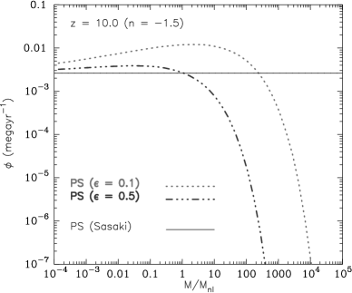
Figure 1: Destruction rate $\phi(M,t)$ at $z=10$ for the Press-Schechter mass function for a power law model with index $-1.5$. Curves have been plotted for $\epsilon=0.1$ and $\epsilon=0.5$.

2.4 Excursion set approach to halo formation rates: Sheth-Tormen mass function

As discussed in Subsection 2.2, the Sheth-Tormen mass function is known to be a much better fit to N-body simulations than the Press-Schechter mass function. Several other forms of halo mass function have also been fitted to results of high resolution N-body simulations (Jenkins et al., 2001; Reed et al., 2003; Warren et al., 2006). In this paper we focus on the Sheth-Tormen mass function. Recall that the Sasaki prescription gave unphysical results when applied to this form of the mass function. Therefore, we now derive the halo destruction rate efficiency, and the halo formation rates for the Sheth-Tormen mass function. This requires obtaining analogs of equations (18) and (19).

Sheth, Mo, & Tormen (2001) showed that once the barrier shape is known, all the predictions of the excursion set approach, like the conditional mass function, associated with that barrier can be computed easily. Further, they showed that the barrier shape for ellipsoidal collapse is

$$B(\sigma,t)\equiv\delta_{\mathrm{ec}}(\sigma,t)=\sqrt{a}\delta_{c}(t)\left[1+\beta(a\nu)^{-\gamma}\right],$$ (21)

where $a=0.75$, $\beta=0.485$, $\gamma=0.615$, and, $\delta_{c}(t)$ is the threshold value of overdensity required for spherical collapse (also see Sheth & Tormen 2002). They also found that, for various barrier shapes $B(S)$, the first-crossing distribution of the excursion set theory is well approximated by

$$f(S)dS=\frac{|T(S)|}{\sqrt{2\pi S^{3/2}}}\exp\left[-\frac{B(S)^{2}}{2S}\right]dS,$$ (22)

where $T(S)$ denotes the sum of the first few terms in the Taylor series expansion of $B(S)$

$$T(S)=\sum\limits_{n=0}^{\infty}\frac{(-S)^{n}}{n!}\frac{\partial^{n}B(S)}{\partial S^{n}}.$$ (23)

(Here, for conformity with the literature, we use the symbol $S\equiv\sigma^{2}$.) This expression gives the exact answer in the case of constant and linear barriers. For the ellipsoidal barrier, we can get convergence of the numerical result if we retain terms in the Taylor expansion up to $n=5$.

For Press-Schechter mass function, the conditional mass function $f(S_{1},\delta_{1}|S_{2},\delta_{2})$ can be obtained from the first crossing $f(S)$ by just changing the variables $\delta\rightarrow\delta_{1}-\delta_{2}$ and $S\rightarrow S_{1}-S_{2}$. This can be done because, despite the shift in the origin, the second barrier is still one of constant height. This is no longer true for Ellipsoidal collapse and hence we cannot simply rescale the function of equation to get the conditional mass function. Instead, this can be done by making the replacements $B(S)\rightarrow B(S_{1})-B(S_{2})$ and $S\rightarrow S_{1}-S_{2}$ in equation (22).

$$\begin{split}f(S_{1}|S_{2})dS_{1}=&\frac{|T(S_{1}|S_{2})|}{\sqrt{2\pi(S_{1}-S_{2})^{3/2}}}\\ &\times\exp\left[-\frac{\left(B(S_{1})-B(S_{2})\right)^{2}}{2(S_{1}-S_{2})}\right]dS_{1},\end{split}$$ (24)

where we now have

$$T(S_{1}|S_{2})=\sum\limits_{n=0}^{5}\frac{(-(S_{1}-S_{2}))^{n}}{n!}\frac{\partial^{n}\left(B(S_{1})-B(S_{2})\right)}{\partial S^{n}_{1}}.$$ (25)

Using Bayes’ theorem, we now have

$$\begin{split}f&\left(S_{2}|S_{1}\right)dS_{2}=\frac{|T(S_{1}|S_{2})||T(S_{2})|}{|T(S_{1})|}\frac{1}{\sqrt{2\pi}}\left[\frac{S_{1}}{S_{2}\left(S_{1}-S_{2}\right)}\right]\\ &\times\exp\left[-\frac{\left[B(S_{1})-B(S_{2})\right]^{2}}{2\left(S_{1}-S_{2}\right)}-\frac{B^{2}(S_{2})}{2S_{2}}+\frac{B^{2}(S_{1})}{2S_{1}}\right]dS_{2}.\end{split}$$ (26)

A change of variables from $S$ to $M$ now gives us an analog of equation (18) for the Sheth-Tormen mass function. In other words, we get the conditional probability $f_{\mathrm{ST}}(M_{2}|M_{1})d\ln M_{2}$ that a halo of mass $M_{1}$ present at time $t_{1}$ will merge to form a halo of mass between $M_{2}$ and $M_{2}+dM_{2}$ at time $t_{2}>t_{1}$. Further, taking the limit as $t_{2}$ tends to $t_{1}(=t)$, we obtain $\tilde{Q}(M_{1},M_{2};t)$. As before, we can then use it to calculate the halo destruction rate efficiency $\phi(M,t)$ and the rate of halo formation $\dot{N}_{\mathrm{form}}^{\mathrm{ST}}(M_{1},z)$ using equations (5) and (20). We perform this part of the calculation numerically. It is also possible to use this formalism to calculate formation rates for the square-root barrier (Moreno, Giocoli, & Sheth, 2009, 2008; Giocoli et al., 2007), which is a good approximation for the ellipsoidal collapse model. We do not attempt this calculation here as it is beyond the scope of this paper.

Fig. 2 is the analog of Fig. 1 for the Sheth-Tormen mass function. It shows the destruction rate per halo $\phi(M,t)$ computed using the excursion set method for an Einstein-de Sitter cosmology with power law spectrum of density perturbations with index $-1.5$ at $z=10.0$. Curves have been plotted for $\epsilon=0.1$ and $\epsilon=0.5$. We have also shown the Sasaki approximation for ST mass function in the same panel for comparison. This result for the Sheth-Tormen mass function has the same features as the result for the Press-Schechter mass function. We also see that the destruction rate efficiency is far from constant at small $M/M_{nl}$. Thus the central assumption of the Sasaki prescription is invalid in the case of Sheth-Tormen mass function as well.

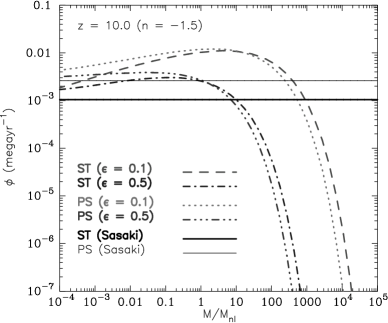
Figure 2: Same as Fig. 1 but for the Sheth-Tormen (as well as Press-Schechter) mass function.

Table 1: For power law: here $n$ is the index of the power spectrum, $N_{\textrm{box}}$ is the size of the simulation box , $N_{\textrm{part}}$ represents the number of particles, $r_{\mathrm{nl}}^{i}$ is the scale of non-linearity at the earliest epoch, $r_{\mathrm{nl}}^{f}$ is the actual scale of non-linearity for the last epoch, $r_{\mathrm{nl}}^{\textrm{max}}$ represents the maximum scale of non-linearity and $z_{i}$ is the starting redshift of the simulations for every model.

$n$	$N_{\mathrm{box}}$	$N_{\mathrm{part}}$	$r_{\mathrm{nl}}^{i}$	$r_{\mathrm{nl}}^{f}$	$r_{\mathrm{nl}}^{\mathrm{max}}$	$z_{i}$
$-1.5$	$400^{3}$	$400^{3}$	$2.5$	$12.0$	$10.0$	$103.38$
$-0.5$	$256^{3}$	$256^{3}$	$2.5$	$12.0$	$18.2$	$291.53$

Table 2: For LCDM: columns 1 and 2 list the size of the box (in Mpc$/h$) and the number of particles used in the simulations. Columns 3 and 4 give the mass (in M${}_{\odot}/h$) and force resolution (in kpc$/h$; not to be confused with the $\epsilon$ used in the text) of the simulations, while columns 5 and 6 tell us the redshift at which the simulations were terminated and the redshift for which the analyses were done.

$L_{\mathrm{box}}$	$N_{\mathrm{part}}$	$m_{\mathrm{part}}$	$\epsilon$	$z_{\mathrm{f}}$	$z_{\mathrm{out}}$
$23.04$	$512^{3}$	$6.7\times 10^{6}$	1.35	5.0	5.04
$51.20$	$512^{3}$	$7\times 10^{7}$	3.00	3.0	3.34
$76.80$	$512^{3}$	$2.3\times 10^{8}$	4.50	1.0	1.33

3 N-body simulations

From the excursion set calculation described in the previous section, we thus find that the halo destruction rate efficiency is not independent of mass as is assumed in the Sasaki prescription. Clearly, this is the reason why Sasaki prescription yields unphysical values for the rate of halo formation. In this section and the next, we now compare the results of our excursion set calculation with results of N-body simulations.

We used the TreePM code (Khandai & Bagla, 2009) for these simulations. The TreePM (Bagla, 2002; Bagla & Ray, 2003) is a hybrid N-body method which improves the accuracy and performance of the Barnes-Hut (BH) Tree method (Barnes & Hut, 1986) by combining it with the PM method (Miller, 1983; Klypin & Shandarin, 1983; Bouchet, Adam, & Pellat, 1985; Bouchet & Kandrup, 1985; Hockney & Eastwood, 1988; Bagla & Padmanabhan, 1997; Merz, Pen, & Trac, 2005). The TreePM method explicitly breaks the potential into a short-range and a long-range component at a scale $r_{s}$: the PM method is used to calculate the long-range force and the short-range force is computed using the BH Tree method. Use of the BH Tree for short-range force calculation enhances the force resolution as compared to the PM method.

The mean interparticle separation between particles in the simulations used here is $l_{\mathrm{mean}}=1.0$ in units of the grid-size used for the PM part of the force calculation. In our notation this is also cube root of the ratio of simulation volume $N_{\mathrm{box}}^{3}$ to the total number of particles $N_{\mathrm{part}}$.

Power law models do not have any intrinsic scale apart from the scale of non-linearity introduced by gravity. We can therefore identify an epoch in terms of the scale of non-linearity $r_{\mathrm{nl}}$. This is defined as the scale for which the linearly extrapolated value of the mass variance at a given epoch $\sigma_{L}(a,r_{\mathrm{nl}})$ is unity. All power law simulations are normalized such that $\sigma^{2}(a=1.0,r_{\mathrm{nl}}=8.0)=1.0$. The softening length in grid units is $0.03$ in all runs.

The $\Lambda$CDM simulations were run with the set of cosmological parameters favored by Wilkinson Microwave Anisotropy Probe 5-yr data (WMAP; Komatsu et al. 2009) as the best fit for the $\Lambda$CDM class of models: $\Omega_{nr}=0.2565,\Omega_{\Lambda}=0.7435,n_{s}=0.963,\sigma_{8}=0.796,h=0.719$ and $\Omega_{b}h^{2}=0.02273$. The simulations were done with $512^{3}$ particles in a comoving cube of three different values of the physical volume as given in Table LABEL:table_nbody_runs_lcdm.

Simulations introduce an inner and an outer scale in the problem and in most cases we work with simulation results where $L_{\mathrm{box}}\gg r_{\mathrm{nl}}\geq L_{\mathrm{grid}}$, where $L_{\mathrm{grid}}$, the size of a grid cell is the inner scale in the problem. $L_{\mathrm{box}}$ is the size of the simulation and represents the outer scale. In Table (LABEL:table_nbody_runs_powlaw) we list the power law models simulated for the present study. We list the index of the power spectrum $n$ (column 1), size of the simulation box $N_{\textrm{box}}$ (column 2), number of particles $N_{\textrm{part}}$ (column 3), the scale of non-linearity at the earliest epoch used in this study (column 4), and, the maximum scale of non-linearity, $r_{\mathrm{nl}}^{\textrm{max}}$ (column 6) given our tolerance level of $3\%$ error in the mass variance at this scale. For some models with very negative indices we have run the simulations beyond this epoch. This can be seen in column 5 where we list the actual scale of non-linearity for the last epoch. The counts of haloes in low mass bins are relatively unaffected by finite box considerations. We therefore limit errors in the mass function by running the simulation up to $r_{\mathrm{nl}}^{\mathrm{max}}$ . Column 7 lists the starting redshift of the simulations for every model. Similarly, in Table (LABEL:table_nbody_runs_lcdm), we mention the details of the LCDM simulations used in this work. We list the size of the simulation box $L_{\mathrm{box}}$ in Mpc$/h$ (column 1), number of particles used in the simulations $N_{\mathrm{part}}$ (column 2), mass of the particles $m_{\mathrm{part}}$ in M${}_{\odot}/h$ (column 3), force resolution $\epsilon$ (not to be confused with the $\epsilon$ used in the text) of the simulations in kpc$/h$ (column 4), the redshift $z_{\mathrm{f}}$ at which the simulations were terminated (column 5) and the redshift $z_{\mathrm{out}}$ for which the analyses were done (column 6).

In order to follow the merger history of dark matter haloes in each of these simulations, we store the particle position and velocities at different redshifts. A friend-of-friend group finding algorithm is used to locate the virialised haloes in each of these slices. We adopt a linking length that is $0.2$ times the mean inter-particle separation, corresponding to the density of virialised haloes. Only groups containing at least $20$ particles are included in our halo catalogs. A merger tree is then constructed out of the halo catalogs by tracking the evolution of each particle through various slices. This lets us identify a halo as it evolves with time through mergers with other haloes. We then describe the formation and destruction of haloes in terms of change in number of particles between consecutive snapshots of the simulation. When a halo of mass $M$ at redshift $z$ turns into a halo of mass $M^{\prime}$ at $z^{\prime}(<z)$, then we say that a halo of mass $M$ was destroyed at redshift $z$ and a halo of mass $M^{\prime}$ has formed at $z^{\prime}$ if $M^{\prime}\geq M(1+\epsilon)$. We identify the resolution parameter $\epsilon$ with that used in our excursion set calculation and experiment with different values as described in the next section.

We find that a tolerence parameter $\epsilon$, similar to the one defined before, also occurs while analysing the results of N-body simulations. We identify these two quantities. As we will see in the next section, the formation rate in our model has a dependence on $\epsilon$, which reproduces the dependence of the results of N-body simulations on this quantity. Thus, the presence of $\epsilon$ in our analytical model is crucial in comparing our results with the N-body results.

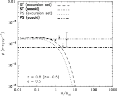
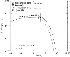
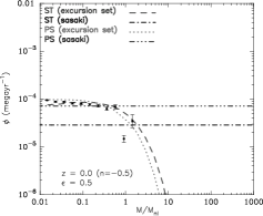
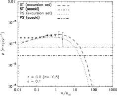
Figure 3: Comparison of the destruction rate efficiencies computed using our method and Sasaki formalism for both ST and PS mass function at $r_{nl}=5$ grid lengths (top row) and $r_{nl}=8$ grid lengths (second row). All curves are plotted for power-law model with index $n=-0.5$. Curves for $\epsilon=0.5$ are shown in the left panel and $\epsilon=0.1$ in the right panel. Points with error bars represent the corresponding results obtained from N-body simulations.

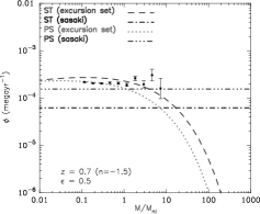
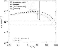
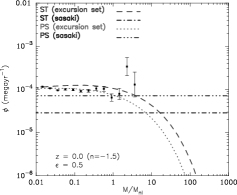
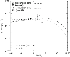
Figure 4: Same as Fig. 3 but now for $n=-1.5$. The two epochs correspond to $r_{nl}=4$ and $r_{nl}=8$ grid lengths respectively.

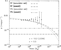
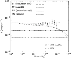
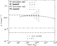
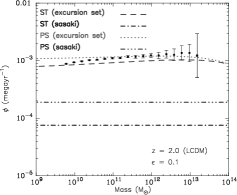
Figure 5: Destruction rates for $\Lambda$CDM model for both PS and ST mass functions using different thresholds ($\epsilon=0.5$ for first; $\epsilon=0.1$ for second) and different redshifts ($z=10.2$ for left panel, $z=2.0$ for right panel). Again, points with error bars represent the corresponding results obtained from N-body simulations.

4 Results and discussion

In this section we present the results of a comparison of our calculations presented in Section 2 with N-body simulations. We present comparison of the destruction rate efficiency and the rate of halo formation and then discuss our results at the end of this section. We also consider two related quantities, the halo survival probability and the distribution of halo formation times, that were defined in Section 2.

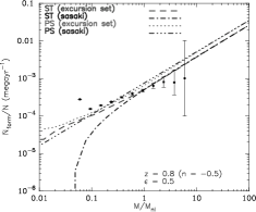
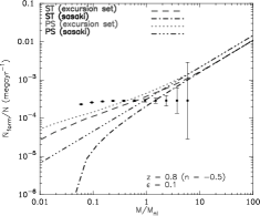
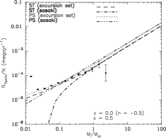
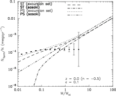
Figure 6: Comparison of the formation rates computed using our method and Sasaki formalism for both ST and PS mass functions for $r_{nl}=5$ (top row) and $r_{nl}=8$ (bottom row). All curves are plotted for power-law model with index $n=-0.5$. Curves for $\epsilon=0.5$ are shown in the left panel and $\epsilon=0.1$ in the right panel. Points with error bars represent the corresponding results obtained from N-body simulations.

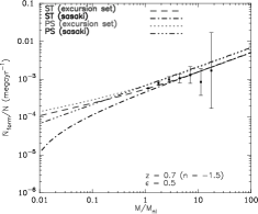
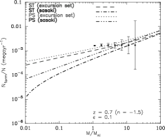
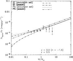
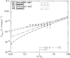
Figure 7: Same as Fig. 6 but now for $n=-1.5$. The two epochs correspond to $r_{nl}=4$ and $r_{nl}=8$ grid lengths respectively.

4.1 Halo destruction rate efficiency

Figs. 3 and 4 show the halo destruction rate efficiency $\phi(M,t)$ for Sheth-Tormen and Press-Schechter mass functions in an Einstein-de Sitter universe with a power law power spectrum of density fluctuations with indices $n=-0.5$ and $n=-1.5$ respectively. The top row of both figures shows the halo destruction rate efficiency at $z=0.8$ and the second row shows the same at $z=0.0$. In each case, we compute the halo destruction rate efficiency using the Sasaki method as well as our excursion set method. We then derive $\phi(M,t)$ from our N-body simulations for a comparison: see Bagla, Khandai & Kulkarni (2009) for details of the simulations and best fit parameters for the ST mass function. These results are superimposed on the plots. For the excursion set calculation and for the comparison with simulations, we use $\epsilon=0.5$ (left column) and $\epsilon=0.1$ (right column). For the two power spectra, the two redshifts that we consider correspond to $r_{\mathrm{nl}}=5$ and $r_{\mathrm{nl}}=8$ grid lengths, and $r_{\mathrm{nl}}=4$ and $r_{\mathrm{nl}}=8$ grid lengths respectively.

As we saw in Figs. 1 and 2, we find that Sasaki’s assumption is not valid for ST or PS mass functions, that is  $\phi(M,t)$ depends on the halo mass. We also see that the value of $\phi(M,t)$ derived from simulations matches well with that calculated by our method. On the other hand, the predictions of Sasaki’s approximation do not match the simulations. This difference is more pronounced for the smaller value of $\epsilon$. Note that the points from N-body simulations have large error-bars at higher mass as the number of haloes decreases at these scales. The most notable feature of the destruction rate efficiency in the excursion set picture is that it cuts off very sharply for large masses. Another aspect is that for small $\epsilon$, there is a pronounced peak in $\phi$ and it drops off towards smaller masses.

We have also calculated the destruction rate efficiency for the $\Lambda$CDM cosmological model for both Press-Schechter and Sheth-Tormen mass functions and compared it with derived values from simulations. The results are shown in Fig. 5 for two redshifts ($2.0$ and $10.2$) and two values of $\epsilon$ ($0.5$ and $0.1$). We can see that results calculated by our technique fit numerical results better.

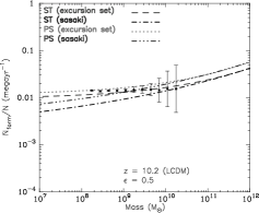
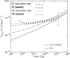
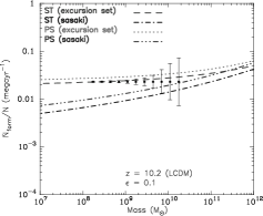
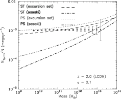
Figure 8: Formation rates for $\Lambda$CDM model for both PS and ST mass functions using different thresholds ($\epsilon=0.5$ for first; $\epsilon=0.1$ for second row) and different redshifts ($z=10.2$ for left panel, $z=2.0$ for right panel). As usual, points with error bars represent the corresponding results obtained from N-body simulations.

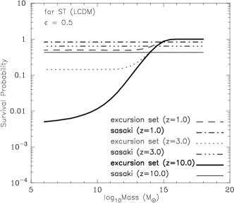
Figure 9: Comparison of the survival probabilities computed using our method and Sasaki formalism for both PS (left panel) and ST (right panel) mass functions with different redshifts ($z=1$, $3$ and $10$) for $\epsilon=0.5$. Curves have been plotted for the $\Lambda$CDM model. These curves show the probability that the halo survives from that redshift up to the present epoch.

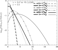
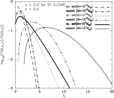
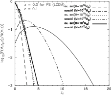
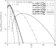
Figure 10: Plots for formation epoch distribution of haloes. Left column is for the PS and the right column is for the ST mass function. Curves have been plotted for the LCDM model. The formation epoch distribution as computed using the Sasaki formalism and the excursion set approach described in this work is shown in the top panel.

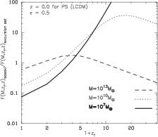
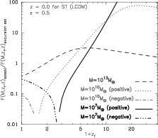
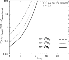
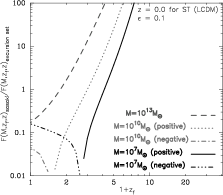
Figure 11: Ratio of the two different approaches used in Fig. 10 to highlight less obvious differences.

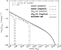
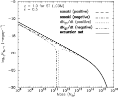
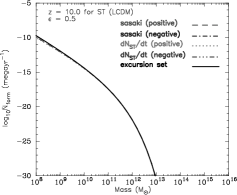
Figure 12: Upper panels show formation rates for ST mass function. Lower panels show the same where we used $\phi$ computed from excursion set approach in the PS mass function and used that to compute the formation rate in the ST mass function.

Figure 13: Ratio of formation rates estimated in the two approaches shown in Fig. 12.

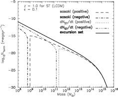
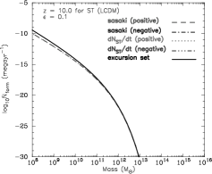
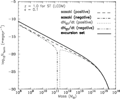
Figure 14: Same as Fig. 12 but for $\epsilon=0.1$

Figure 15: Same as Fig. 13 but for $\epsilon=0.1$

4.2 Halo formation rate

Having calculated the destruction rate efficiency, we can now calculate the halo formation rate using the formalism described in Section 2 and compare it with the derived halo formation rates from our simulations. The results are shown in Figs. 6 and 7 for an Einstein-de Sitter Universe with a power law power spectrum of density fluctuations with indices $n=-0.5$ and $n=-1.5$ respectively. The third row of both figures shows the formation rate at redshift $z=0.8$ and the fourth row shows the same at redshift $z=0.0$. Note the quantity plotted here is the ratio $\dot{N}_{\mathrm{form}}(M,t)/N(M,t)$. We have shown the results from the Sasaki prescription and the excursion set calculations and have superimposed formation rates derived from N-body simulations. As before, for the excursion set calculation and for the comparison with simulations, we use $\epsilon=0.5$ (left column) and $\epsilon=0.1$ (right column). For the two power spectra, the two redshifts that we consider correspond to $r_{\mathrm{nl}}=5$ and $r_{\mathrm{nl}}=8$ grid lengths, and $r_{\mathrm{nl}}=4$ and $r_{\mathrm{nl}}=8$ grid lengths respectively. The corresponding results for the $\Lambda$CDM cosmological model are shown in Fig. 8 for two redshifts (2.0 and 10.2) and two values of $\epsilon$ (0.5 and 0.1).

Again, we see that the excursion set results fit simulation data much better as compared to the results from Sasaki prescription. The Sasaki method underestimates the formation rates by a large factor for low mass haloes. Results from the two methods tend to converge in the large mass limit, although a systematic difference remains between the Sheth-Tormen and Press-Schechter estimates, with the former always being larger that the later. The difference in the Sasaki estimate and the excursion set estimate for the destruction rate efficiency and the formation rate is as high as an order of magnitude at some scales so the close proximity of simulation points to the excursion set calculations is a clear vindication of our approach. It is worth noting that there is a clear deviation of simulation points from the theoretical curves at small mass scales and this deviation is more pronounced at small mass scales for $\epsilon=0.5$. It may be that some of the deviations arise due to a series representation of the barrier shape, and the number of terms taken into account may not suffice for the estimate. We have found that truncation of the series can affect results at small masses, though in most cases results converge with the five terms that we have taken into account for the range of masses considered here.

4.3 Halo survival probability

An important auxiliary quantity in the ongoing discussion is the halo survival probability, defined in Section 2. From our calculation of the halo destruction rate efficiency, we calculated the survival probability of dark matter haloes using both the excursion set formalism and the Sasaki prescription and compared results. These results are shown in Fig. 9, which shows the survival probabilities in the $\Lambda$CDM cosmological model for the Press-Schechter (left panel) and Sheth-Tormen (right panel) mass functions using the two approaches at three different redshifts ($z=1$, $3$ and $10$). In this case, we have used $\epsilon=0.5$ for the excursion set calculation.

In Sasaki approximation, the destruction rate is independent of mass and hence the survival probability is also independent of mass. Our calculations show that this approximation is not true, and hence the survival probability of haloes must also depend on mass. We note that the survival probability is high for large mass haloes: if a very large mass halo forms at a high redshift then it is likely to survive without a significant addition to its mass. Smaller haloes are highly likely to merge or accrete enough mass and hence do not survive for long periods. Survival probability drops very rapidly as we go to smaller masses. While this is expected on physical grounds, it is an aspect not captured by the Sasaki approximation where equal survival probability is assigned to haloes of all masses. The mass dependence of survival probability is qualitatively similar to that obtained by Kitayama & Suto (1996). There is no significant qualitative difference between the curves for the Press-Schechter and the Sheth-Tormen mass functions.

4.4 Formation time distribution

Finally, another interesting quantity is the distribution $F(M;t_{f},t)$ of formation epochs $t_{f}$ of haloes with mass $M$ at $t$, defined in Section 2. This distribution can be obtained once the survival probability and formation rate of haloes is known. We calculated the formation time distribution using the excursion set formalism and the Sasaki prescription. The results are shown in Fig. 10. We plot $F(M;z_{f},z=0)/N(M,z=0)$ versus the formation redshift $z_{f}$ for three different masses ($10^{13}$, $10^{10}$ and $10^{7}M_{\odot}$) in the standard $\Lambda$CDM model for both Press-Schechter (left column) and Sheth-Tormen (right column) mass functions with $\epsilon=0.5$ (first row) and $\epsilon=0.1$ (second row). A common feature is that $F$ as a function of $z_{f}$ increases up to a certain redshift and then starts to decline. The epochs at which $F$ drops by an order of magnitude from its peak can be interpreted as typical range of redshifts for the formation of bound systems of respective masses which exist at $z=0$.

The differences between the formation redshift distribution for $\epsilon=0.5$ and $\epsilon=0.1$ are along expected lines: the formation redshifts are smaller for the lower value of $\epsilon$ as a smaller change in mass is required for us to declare that a new halo has formed and hence typical haloes do not survive for a very long time. We see that the excursion set calculation suggests that haloes formed more recently as compared to the Sasaki approximation based estimate. This can be understood in terms of the equal survival probability assigned by the Sasaki approximation to haloes of all masses. For a clearer comparison, the ratio of the estimate based on Sasaki approximation and the excursion set calculation is shown in Fig. 11. We note that for very low mass haloes these two estimates differ by more than an order of magnitude. The main qualitative difference between the plots for the Press-Schechter and the Sheth-Tormen mass functions is caused by the negative formation rates in the Sasaki approximation.

4.5 Discussion

The results described above show conclusively that the excursion set approach predicts halo formation and destruction rates that match with simulations much better than the Sasaki approximation.

Another noteworthy aspect is that the destruction and formation rates depend on the value of $\epsilon$ in simulations as well as the excursion set calculation thereby allowing us to differentiate between major and minor mergers. In comparison, there is no natural way to bring in this dependence in the Sasaki approximation. While the match between simulations and the excursion set approach for the two values of $\epsilon$ is satisfying, it raises the question of the appropriate value of this parameter. In our view the appropriate value of the parameter should depend on the application in hand. In semi-analytic galaxy formation models, we should use a value of $\epsilon$ that corresponds to the smallest ratio of masses of the infalling galaxy and the host galaxy where we expect a significant dynamical influence on star formation rate. For instance, Kauffmann et al. (1999) use $\epsilon=0.3$ in their semi-analytic galaxy formation model while considering formation of bulges in merger remnants. In case of galaxy clusters we may base this on the smallest ratio of masses where the intra-cluster medium is likely to be disturbed in a manner accessible to observations in X-ray emission or the Sunyaev-Zel’dovich effect (Sunyaev & Zeldovich, 1972; Navarro, Frenk, & White, 1995; Kay, 2004).

While the close match between simulations and the excursion set calculation is useful, it also implies that we should not use the simpler Sasaki approximation. The excursion set calculation of the halo destruction rate is fairly simple for the Press-Schechter mass function, but the corresponding calculation for the Sheth-Tormen mass function is much more complicated. Plots of the destruction rate efficiency $\phi(M)$ for all the models suggest that its variation with mass and $\epsilon$ is very similar for the PS and ST mass function. This suggests an approximation where we use $\phi(M,z;\epsilon)$ computed using the Press-Schechter mass function and use that to compute the halo formation rate in the Sheth-Tormen mass function. Figs. 12 and 14 show the halo formation rate for the $\Lambda$CDM model at different redshifts and compare the excursion set calculation, the Sasaki approximation and the intermediate approximation suggested above. We have also shown the ratios of formation rates estimated in these two approaches mentioned above in Figs. 13 and 15. We find that the intermediate approximation is not plagued by negative halo formation rates and that it is an excellent approximation at all mass scales at higher redshifts. At lower redshifts, the approximation is still good at high masses but not so at smaller masses.

While comparing our analytical results with those of N-body simulations, we find a systematic deviation between the two at the high mass end. This is possibly related to the problm of ‘halo fragmentation’ while deriving halo merger trees from the simulations. In about 5% of all haloes, particles in a given progenitor halo can become part of two independent haloes at a future epoch. This is usually attributed to the fact that the FOF algorithm groups particles based on the inter-particle distance. This can result in the identification of two haloes separated by a thin ’bridge’ of particles to be treated as a single halo. Such halo fragmentation has been treated using different techniques in various halo formation rate studies. Fakhouri & Ma (2008) compare these techniques and find that the effect of halo fragmentation is maximum of high mass haloes.

5 Conclusions

Key points presented in this paper can be summarized as follows:

• We revisit the Sasaki approximation for computing the halo formation rate and compute the destruction rate explicitly using the excursion set approach.

• We introduce a parameter $\epsilon$, the smallest fractional change in mass of a halo before we consider it as destruction of the old halo and formation of a new halo.

• We show that the halo destruction rate is not independent of mass even for power law models and hence the basis for the Sasaki ansatz does not hold. Two prominent features of the halo destruction rate are the rapid fall at large masses, and a pronounced peak close to the scale of non-linearity. The peak is more pronounced for smaller values of $\epsilon$.

• Using the excursion set approach for the Sheth-Tormen mass function leads to positive halo formation rates, unlike the generalization of the Sasaki ansatz where formation rates at some mass scales are negative.

• We compare the destruction rate and the halo formation rates computed using the excursion set approach with N-body simulations. We find that our approach matches well with simulations for all models, at all redshifts and also for different values of $\epsilon$.

• In some cases there are deviations between the simulations and the theoretical estimate. However, these deviations are much smaller for the excursion set based method as compared to the Sasaki estimate.

• It may be that some of the deviations arise due to a series representation of the barrier shape, and the number of terms taken into account may not suffice for the estimate. We have found that truncation of the series can affect results at small masses, though in most cases results converge with the five terms that we have taken into account for the range of masses considered here.

• We show that we can use the halo destruction rate computed for the Press-Schechter mass function to make an approximate estimate of the halo formation rate in Sheth-Tormen mass function using equation (5). This approximate estimate is fairly accurate at all mass scales in the $\Lambda$CDM model at high redshifts.

• The halo survival probability is a strong function of mass of haloes, unlike the mass independent survival probability obtained in the Sasaki approximation.

• The halo formation redshift distribution for haloes of different masses is also very different from that obtained using the Sasaki approximation. This is especially true for the Sheth-Tormen mass function where the Sasaki approximation gives negative halo formation rates in some range of mass scales and redshifts.

The formalism used here for calculation of halo formation rate and other related quantities can be generalized to any description of the mass function if the relevant probabilities can be calculated. Within the framework of the universal approach to mass functions, it can also be used to study formation rates of haloes in different cosmological models (Linder & Jenkins, 2003; Macciò et al., 2004). This allows for an easy comparison of theory with observations for quantities like the major merger rate for galaxy clusters (Cohn, Bagla, & White, 2001).

In case of semi-analytic models of galaxy formation, our approach allows for a nuanced treatment where every merger need not be treated as a major merger and we may only consider instances where mass ratios are larger than a critical value for any affect on star formation in the central galaxy.

References

- Bagla (2002) Bagla J. S., 2002, JApA, 23, 185
- Bagla & Padmanabhan (1997) Bagla J. S., Padmanabhan T., 1997, Pramana, 49, 161
- Bagla & Ray (2003) Bagla J. S., Ray S., 2003, NewA, 8, 665
- Bagla, Khandai & Kulkarni (2009) Bagla J. S., Khandai N., Kulkarni G., 2009, arXiv0908.2702
- Barnes & Hut (1986) Barnes J., Hut P., 1986, Nature, 324, 446
- Benson et al. (2005) Benson A. J., Kamionkowski M., Hassani S. H., 2005, MNRAS, 357, 847
- Bernardeau et al. (2002) Bernardeau F., Colombi S., Gaztañaga E., Scoccimarro R., 2002, PhR, 367, 1
- Binney (1977) Binney J., 1977, ApJ, 215, 483
- Blain & Longair (1993) Blain A.W., Longair M.S. 1993, MNRAS, 264, 509
- Bond et al. (1991) Bond J. R., Cole S., Efstathiou G., Kaiser N., 1991, ApJ, 379, 440
- Bouchet & Kandrup (1985) Bouchet F. R., Kandrup H. E., 1985, ApJ, 299, 1
- Bouchet, Adam, & Pellat (1985) Bouchet F. R., Adam J.-C., Pellat R., 1985, A&A, 144, 413
- Chandrasekhar (1943) Chandrasekhar S., 1943, RvMP, 15, 1
- Chiu & Ostriker (2000) Chiu W. A., Ostriker J. P., 2000, ApJ, 534, 507
- Choudhury & Ferrara (2005) Choudhury T. R., Ferrara A., 2005, MNRAS 361, 577
- Cohn & White (2008) Cohn J. D., White M., 2008, MNRAS, 385, 2025
- Cohn, Bagla, & White (2001) Cohn J. D., Bagla J. S., White M., 2001, MNRAS, 325, 1053
- De Simone, Maggiore, & Riotto (2011) De Simone A., Maggiore M., Riotto A., 2011, MNRAS, in press (arXiv:1102.0046)
- Efstathiou et al. (1988) Efstathiou G., Frenk C. S., White S. D. M., Davis M., 1988, MNRAS, 235, 715
- Fakhouri & Ma (2008) Fakhouri O., Ma C.-P., 2008, MNRAS, 386, 577
- Fakhouri, Ma, & Boylan-Kolchin (2010) Fakhouri O., Ma C.-P., Boylan-Kolchin M., 2010, MNRAS, 406, 2267
- Giocoli et al. (2007) Giocoli C., Moreno J., Sheth R. K., Tormen G., 2007, MNRAS, 376, 977
- Gunn & Gott (1972) Gunn J. E., Gott J. R. I., 1972, ApJ, 176, 1
- Hockney & Eastwood (1988) Hockney R. W., Eastwood J. W., 1988, Computer Simulation using Particles, McGraw-Hill
- Hoyle (1953) Hoyle F., 1953, ApJ, 118, 513
- Jenkins et al. (2001) Jenkins A., Frenk C. S., White S. D. M., Colberg J. M., Cole S., Evrard A. E., Couchman H. M. P., Yoshida N., 2001, MNRAS, 321, 372
- Kauffmann, White & Guiderdoni (1993) Kauffmann, G., White, S. D. M., Guiderdoni, B., 1993, MNRAS, 264, 201
- Kauffmann et al. (1999) Kauffmann G., Colberg J. M., Diaferio A., White S. D. M., 1999, MNRAS, 303, 188
- Kay (2004) Kay S. T., 2004, MNRAS, 347, L13
- Khandai & Bagla (2009) Khandai N., Bagla J. S., 2009, Research in Astronomy and Astrophysics, 9, 861
- Kitayama & Suto (1996) Kitayama T., Suto Y., 1996, MNRAS, 280, 638
- Klypin & Shandarin (1983) Klypin A. A., Shandarin S. F., 1983, MNRAS, 204, 891
- Komatsu et al. (2009) Komatsu E., et al., 2009, ApJS, 180, 330
- Lacey & Cole (1993) Lacey C., Cole S., 1993, MNRAS, 262, 627
- Lacey & Cole (1994) Lacey C., Cole S., 1994, MNRAS, 271, 676
- Li et al. (2007) Li Y., Mo H. J., van den Bosch F. C., Lin W. P., 2007, MNRAS, 379, 689
- Linder & Jenkins (2003) Linder E. V., Jenkins A., 2003, MNRAS, 346, 573
- Lukić et al. (2007) Lukić Z., Heitmann K., Habib S., Bashinsky S., Ricker P. M., 2007, ApJ, 671, 1160
- Macciò et al. (2004) Macciò A. V., Quercellini C., Mainini R., Amendola L., Bonometto S. A., 2004, PhRvD, 69, 123516
- Madau, Ferrara, & Rees (2001) Madau, P., Ferrara, A., Rees, M., 2001, ApJ, 555, 92
- Merz, Pen, & Trac (2005) Merz H., Pen U. L., Trac H., 2005, NewA, 10, 393
- Miller (1983) Miller R. H., 1983, ApJ, 270, 390
- Moreno, Giocoli, & Sheth (2009) Moreno J., Giocoli C., Sheth R. K., 2009, MNRAS, 397, 299
- Moreno, Giocoli, & Sheth (2008) Moreno J., Giocoli C., Sheth R. K., 2008, MNRAS, 391, 1729
- Navarro, Frenk, & White (1995) Navarro J. F., Frenk C. S., White S. D. M., 1995, MNRAS, 275, 720
- Neistein & Dekel (2008) Neistein E., Dekel A., 2008, MNRAS, 388, 1792
- Neistein, Maccio & Dekel (2010) Neistein E., Maccio Andrea V., Dekel A., 2010, MNRAS, 403, 984
- Padmanabhan (2002) Padmanabhan T., 2002, Theoretical Astrophysics, Volume III: Galaxies and Cosmology. Cambridge University Press.
- Peacock (1999) Peacock J. A., 1999, Cosmological Physics, Cambridge University Press
- Peebles (1980) Peebles P. J. E., 1980, The Large-Scale Structure of the Universe, Princeton University Press
- Percival (2001) Percival W. J., 2001, MNRAS, 327, 1313
- Percival & Miller (1999) Percival W., Miller L., 1999, MNRAS, 309, 823
- Percival, Miller, & Peacock (2000) Percival W. J., Miller L., Peacock J. A., 2000, MNRAS, 318, 273
- Porciani et al. (1998) Porciani C., Matarrese S., Lucchin F., Catelan P., 1998, MNRAS, 298, 1097
- Press & Schechter (1974) Press W. H., Schechter P., 1974, ApJ, 187, 425
- Reed et al. (2003) Reed D., Gardner J., Quinn T., Stadel J., Fardal M., Lake G., Governato F., 2003, MNRAS, 346, 565
- Reed et al. (2007) Reed D. S., Bower R., Frenk C. S., Jenkins A., Theuns T., 2007, MNRAS, 374, 2
- Rees & Ostriker (1977) Rees M. J., Ostriker J. P., 1977, MNRAS, 179, 541
- Ripamonti (2007) Ripamonti E., 2007, MNRAS, 376, 709
- Samui et al. (2007) Samui S., Srianand R., Subramanian K., 2007, MNRAS 377, 285.
- Samui et al. (2009) Samui S., Subramanian K., Srianand R., 2009, New Astron., 14, 591
- Sasaki (1994) Sasaki S., 1994, PASJ, 46, 427
- Shandarin & Zeldovich (1989) Shandarin S. F., Zeldovich Y. B., 1989, RvMP, 61, 185
- Sheth & Tormen (1999) Sheth R. K., Tormen G., 1999, MNRAS, 308, 119
- Sheth & Tormen (2002) Sheth R. K., Tormen G., 2002, MNRAS, 329, 61
- Sheth, Mo, & Tormen (2001) Sheth R. K., Mo H. J., Tormen G., 2001, MNRAS, 323, 1
- Silk (1977) Silk J., 1977, ApJ, 211, 638
- Sunyaev & Zeldovich (1972) Sunyaev R. A., Zeldovich Y. B., 1972, CoASP, 4, 173
- Tinker et al. (2008) Tinker J., Kravtsov A. V., Klypin A., Abazajian K., Warren M., Yepes G., Gottlöber S., Holz D. E., 2008, ApJ, 688, 709
- Trimble (1987) Trimble V., 1987, ARA&A, 25, 425
- Warren et al. (2006) Warren M. S., Abazajian K., Holz D. E., Teodoro L., 2006, ApJ, 646, 881
- White & Frenk (1991) White S. D. M., Frenk C. S., 1991, ApJ, 379, 52
- White (2002) White M., 2002, ApJS, 143, 241
- Zentner (2007) Zentner A. R., 2007, Int. J. Modern Phys. D, 16, 763