Improved Edge Awareness in
Discontinuity Preserving Smoothing

Abstract

Discontinuity preserving smoothing is a fundamentally important procedure that is useful in a wide variety of image processing contexts. It is directly useful for noise reduction, and frequently used as an intermediate step in higher level algorithms. For example, it can be particularly useful in edge detection and segmentation. Three well known algorithms for discontinuity preserving smoothing are nonlinear anisotropic diffusion, bilateral filtering, and mean shift filtering. Although slight differences make them each better suited to different tasks, all are designed to preserve discontinuities while smoothing. However, none of them satisfy this goal perfectly: they each have exception cases in which smoothing may occur across hard edges. The principal contribution of this paper is the identification of a property we call edge awareness that should be satisfied by any discontinuity preserving smoothing algorithm. This constraint can be incorporated into existing algorithms to improve quality, and usually has negligible changes in runtime performance and/or complexity. We present modifications necessary to augment diffusion and mean shift, as well as a new formulation of the bilateral filter that unifies the spatial and range spaces to achieve edge awareness.

1 Introduction

Discontinuity preserving algorithms attempt to smooth an image while preserving crisp edges. They are useful for many tasks, such as noise reduction, edge detection, and segmentation. Some very robust results have been obtained by treating the smoothing process as a global optimization problem, where the objective is to recover a smooth image that has high fidelity to the original corrupted image. Typically, the energy function to be minimized is a summation over all pixels in the image with two terms, one of which is minimized by a perfectly smooth image, and the other by perfect fidelity to the original corrupted image.

It has been shown that the solution that minimizes such a function is also the maximal a posteriori solution to the problem, as defined by the prior and data terms [9] [7] [13]. Although this is an NP-hard [10] non-convex optimization problem [11], many novel algorithms have been proposed which can efficiently find good global minima in polynomial time, including Mean Field Annealing (MFA) [9] [7] [22] [21], Graduated Non-Convexity (GNC) [12], Belief Propagation (BP) [13], and Graph Cuts (GC) [14] [15] [16]. Earlier works have also identified specific line and outlier processes, further discussed in [11].

However, the global approaches have some significant disadvantages: they are often difficult to generalize to vector-valued images, they are generally very inefficient, they often have trouble maintaining perfectly smooth gradients, and fine structure may be lost.

In this paper, a few algorithms are discussed which have emerged as some popular efficient alternatives to global optimization. The algorithms we consider are variable conductance diffusion [17] [18] [19] [7] [20], bilateral filtering [8] [20], and mean shift filtering [3].

An example of filtering using each of these methods on the noisy Apollo image is shown in Fig. 1. As can be seen from this test image, each method can be effectively used to reduce noise while preserving sharp edges. Although these algorithms perform the same fundamental task, there is no clear winner between them – they all perform well, and individual differences between them (discussed in more detail in the following sections) are significant enough that each has found a niche where it may be superior to the others.

(a) Original

(b) Diffusion

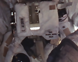
(c) Bilateral

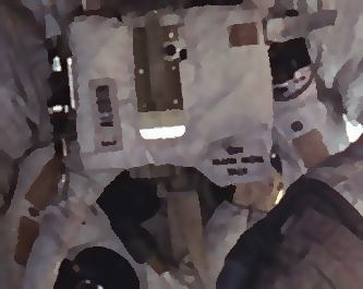
(d) Mean shift

Figure 1: Original (a) and filtered result of Apollo image using: (b) 5 iterations of diffusion with $\lambda=0.03$; (c) regular bilateral filter with $\sigma_{S}=3$, $\sigma_{R}=45$; (d) regular mean shift filter with $h_{s}=5$ and $h_{r}=45$.

The mean shift filter produces more crisp lines in homogeneous regions because it was originally designed for a somewhat ulterior purpose – it is an adaptation of mean shift clustering for fine-scale segmentation of color images. Thus, smooth gradients are avoided, because pixel colors represent segments, and it is only a coincidence that this also appears to be an effective mechanism for discontinuity preserving smoothing.

The bilateral filter and diffusion methods appear to produce results of similar quality, but they are not equal; the bilateral filter can produce a greater contrast between sharp edges and very smooth regions, and is more efficient on massively parallel architectures. Conversely, diffusion is more efficient on single processor machines, and has a more physically meaningful result because it closely approximates the physical diffusion of densities through a medium.

We make no attempt to compare or rank the aforementioned algorithms against each other. However, we have noticed that that there are certain limitations to each algorithm which can result in unwanted effects, and examples of these issues are demonstrated on a specially designed Challenge test image, shown in Fig. 2.

There are several notable features of this test image. In the upper region, there is a gradient going from the white background to a solid red color, adjacent to an orange rectangle, which is separated by a thin black line. Because the red and orange regions are clearly separated, we claim that smoothing should not occur across these regions.

In the bottom half of the image there are four black rectangles each containing noise with a different dominant color: red, green, yellow, or purple. We claim that a smoothing algorithm should reduce the noise within these rectangles leaving each one filled with a solid color, and also preserve the crisp edges of the rectangles.

Surrounding the rectangles is more brightly colored noise, but the noise is not uniform – the area is divided into blobs with distinctly dominant colors. We claim that a smoothing algorithm should reduce this to a smoothly varying colored surface.

In the right region, there are 6 distinctly colored rectangles containing low levels of zero-mean noise. This presents a particularly simple task for a discontinuity preserving smoothing algorithm, and is shown here as somewhat of a control.

(a) Original

(b) Diffusion

(c) Bilateral

(d) Mean shift

Figure 2: Synthetic Challenge (a) test image exhibiting some properties that cause existing methods to perform poorly: (b) variable conductance diffusion blurs hard edges (intentionally exaggerated here for illustration purposes); (c) the bilateral filter loses saturation and fails to smooth in high-noise regions; (d) mean shift mangles some of the edges.

From Fig. 2b, we see that successive iterations of diffusion erodes even the hardest edges, due to the Gaussian blurring of derivatives (we have used a blurring radius that makes this effect noticeable, although it could be tweaked to produce a nicer image). From Fig. 2c, we see that the bilateral filter reduces saturation, produces an unwanted new color by blending the red and orange sections, and has trouble smoothing the highly noisy colored areas. From Fig. 2d, we see that the mean shift filter mangles the black border edge features.

In this paper, we investigate the cause of these unwanted effects, and show that most of them can be related to the violation of a certain principle which we refer to as edge awareness. We propose modifications to correct each algorithm with little or no changes in time complexity, and demonstrate that these modifications can significantly improve visual quality of smoothing. Specifically, we will show that

1. Edge awareness is a concept that can be used to reduce estimation bias in image restoration.

2. Diffusion is naturally edge aware, but becomes progressively less so with each iteration. This can be fixed to preserve crisp edges after successive iterations, at minor additional expense and no change in time complexity (as shown in Section 6).

3. Edge awareness can be incorporated into the concept of the bilateral filter in a very intuitive way to produce a novel algorithm that unifies the spatial and range spaces. Our modification multiples the time complexity as compared to a standard bilateral filter by $O(\log d)$, for a neighborhood of size $d$ (as shown in Section 7).

4. Edge awareness can be partially incorporated into the mean shift filter with minimal change in running time by preventing mean shift paths from crossing strong intensity boundaries (as shown in Section 8). This prevents unwanted artifacts from appearing.

2 Edge Awareness

In order to be called discontinuity or edge preserving, a smoothing algorithm needs only to smooth areas without edges more than the areas with edges. This leaves considerable flexibility in interpretation, and many algorithms satisfying this criterion exist. However, we argue that a more restrictive criterion may be better used to describe an unbiased discontinuity preserving smoothing algorithm, which we refer to as edge awareness.

Specifically, the criterion for edge awareness is:

The influence that a pixel in the input image has on the output at another pixel location should be inversely related to the strength of the largest edge(s) separating those pixels in the input image.

This criterion has statistical rationale behind it for noise removal. The process of smoothing can be equated to estimating the sample mean of the color reflectance distribution at each pixel, and discontinuities in an image are reliable indicators of a change in the underlying reflectance distribution. Without any a priori knowledge of the distributions contained within an image, disjoint regions must be assumed to come from disjoint distributions, and samples from one distribution cannot possibly help in estimating the mean of another distribution. Therefore, pixels which are separated by a discontinuity, and hence not likely to come from the same distribution, should not influence each other.

Arguably, there are many cases where a single reflectance distribution could be responsible for generating samples at disconnected regions in the image. For example, in the regions separated by veins in a leaf, or the out of focus background in a photograph separated by occluding foreground objects (see images A and B in Fig. 3). In these cases the quality of the sample mean could be improved by using the samples from both distributions (eg, smoothing between disjoint regions).

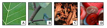
Figure 3: Color distributions in real images: (a) the veins of a leaf separate regions of green having the same underlying distribution; (b) a foreground twig separates regions of a background out-of-focus, having a uniform distribution; (c) a crowd of people with many similar but differently colored body parts; (d) a collection of buttons with similar but different distributions of red.

However, an unbiased smoothing algorithm should not assume that two distributions are the same just because their sample means are similar, because this is frequently not the case. As an example, consider a crowd of people: people tend to have similar skin colors which could appear close together in the image, but a smoothing algorithm should not change a person’s skin color by blending them together (see examples C and D in Fig. 3).

A smoothing algorithm that is not edge aware imposes the additional, often unwanted, assumption that distributions having similar means are the same distribution. Doing so can result in the creation of novel colors that did not exist in the original image, which is counter productive if the purpose of smoothing is to recover a better estimate of the underlying process by removing noise (as it frequently is).

3 Variable Conductance Diffusion

Variable conductance diffusion [17] [18] [19] [7] [20] has long been used as a method of discontinuity preserving smoothing for images. It is inspired by the diffusion equation (3.1), and uses a heuristic measure of conductivity $c$ that is somehow based on the local image derivative magnitude.

$$\frac{\partial f(x,y)}{\partial t}=\nabla\cdot(C(x,y)\nabla f(x,y))$$ (3.1)

For gray level images, the diffusion equation directly translates into an iterative discontinuity preserving smoothing algorithm using finite difference approximations to the derivatives, where $f(x,y)$ is image intensity, and conductivity is a decreasing function of local gradient magnitude [20] [19],

$$C(x,y)=g(||\nabla f(x,y)||)$$ (3.2)

In our implementation, we deviate slightly by using a vector-valued conductivity,

$$\begin{split}\frac{\partial f(x,y)}{\partial t}&=\nabla\cdot(C(x,y)^{\mathsf{T}}\nabla f(x,y))\\ &=\frac{\partial}{\partial x}\left(c_{x}(x,y)\frac{\partial f(x,y)}{\partial x}\right)+\frac{\partial}{\partial y}\left(c_{y}(x,y)\frac{\partial f(x,y)}{\partial y}\right)\end{split}$$ (3.3)

and we make smoothing in each dimension a function of the partial derivative, so that $C(x,y)=[c_{x}(x,y)c_{y}(x,y)]^{\mathsf{T}}$. The components $c_{x}(x,y)$ (and correspondingly $c_{y}(x,y)$) are defined by

$$c_{x}(x,y)=\exp\left(-\lambda||\frac{\partial f(x,y)}{\partial x}||^{2}\right)$$ (3.4)

For color images, the conductance in each channel can be made a function of the overall intensity gradient. Alternatively, Sapiro & Ringach [6] have proposed a method based on the local structure tensor.

VCD is sometimes confused with anisotropic diffusion, which is almost identical but explicitly diffuses in the direction tangent to the local edge [7]. In practice, all of these diffusion methods have similar performance.

The diffusion process attempts to smooth in a way that respects intensity boundaries by making the amount of smoothing related to the magnitude of the derivatives. As a result, colors should not be blurred together unless there exists some path between them that does not significantly go against any local image gradients. Therefore, diffusion is edge aware in theory.

3.1 Limitations of Diffusion

Finite differences are first order approximations of the true derivative, and iterative use causes these approximation errors to become magnified. One way to help mitigate this problem is to alternate between the causal and non-causal forms of the derivative on each iteration. However, noisy images may contain a large degree of high frequency content so that this is generally not enough to eliminate artifacts.

In practice, a Gaussian blurring step is used before computing the finite difference derivative approximations [6]. This naturally makes the derivatives more stable by considering a slightly lower frequency. If noise is mostly high frequency, this also makes the derivatives more representative of the underlying signal.

Unfortunately, because edges are inherently high frequency, lower frequency derivatives will not be able to accurately represent crisp edges, which will lead to slight blurring of edges with each iteration (as in Fig. 2b). Although this blurring effect can be mitigated by using a very small sigma, it will always be present. Thus, the algorithm becomes progressively less aware of edges/discontinuities with each iteration, and will eventually break down and converge to smoothing everywhere. In this paper, we intentionally use a blurring sigma that is large enough to be noticeable.

4 The Bilateral Filter

The bilateral filter was developed by Tomasi & Manduchi for discontinuity preserving smoothing as a non-iterative alternative to anisotropic diffusion [8]. The primary claim for improvement over anisotropic diffusion is that the iterations in diffusion raise issues of stability, as small errors in the derivative estimation can become magnified over time, producing a less smooth image. Additionally, iterative algorithms can be inefficient for massively parallel architectures with limited communication.

The bilateral filter overcomes these issues by considering a single fixed neighborhood of influence around each pixel, and estimating the influence of each neighbor by a combined spatial and range weighting. Specifically, each output pixel is replaced by a doubly-weighted average using the spatial distance and range (color) distance of the original neighbors. For each pixel coordinate $s$, the output color $J_{s}$ is given by

$$J_{s}=\frac{1}{k}\sum_{p\in\Omega}f(||p-s||)g(||I_{p}-I_{s}||)I_{p}$$ (4.1)

where $\Omega$ is the set of image pixels, $I_{p}$ is the RGB intensity at pixel $p$ in the input image $I$, and $k$ is a normalization term. $f$ and $g$ could be any 1D kernel functions, but in practice $g$ is a true Gaussian with standard deviation $\sigma_{R}$ and $f$ is a truncated Gaussian (for computational efficiency) with standard deviation $\sigma_{S}$.

Because it is not iterative and does not rely on derivatives, this makes it more numerically stable, but the use of large overlapping neighborhoods is also much more inefficient; unlike the Gaussian blur, this filter cannot be separated into a horizontal and vertical pass for increased efficiency.

4.1 Limitations of the Bilateral Filter

The bilateral filter is completely unaware of edges because neighboring pixels are averaged together based only on their color similarity, with no regard to any edges that might be separating them. As the spatial radius gets larger, the likelihood of two similarly colored pixels in the neighborhood being separated by some kind of discontinuity grows very quickly. This results in blurring across edges. In addition to producing novel colors, this can produce oddly surrealistic effects because it often blurs the interior of foreground objects with the background, as if it were a line drawing.

Even if the foreground and background colors are noticeably different, a high noise content may necessitate using a large color bandwidth, so that these colors are still blurred, resulting in noticeable color bleeding across boundaries. Also, opposing bright colors with similar intensity may be blurred together, resulting in muted grays and browns instead of the original vibrant colors (this is demonstrated by the noisy background in Fig. 2). This effect will be referred to as color cancellation, and results in loss of saturation.

Some images are more prone to these issues than others. If an image does not contain nearby opposing colors, has a sparse histogram, or has a very high signal to noise ratio, then the bilateral filter may producing very visually appealing results. However, this does not always mean that the results are accurate, because color bleeding across boundaries will still result in changing the average colors even if they still look good to a human.

It should be noted that, in some contexts, blurring across boundaries is considered an advantage rather than a limitation. For example, if the objective is to generate a cartoon-like image rather than produce a realistic smoothing.

5 The Mean Shift Filter

Mean shift clustering [3] was originally developed as a method of clustering multi-dimensional data using an iterative hill-climbing technique to assign each pattern to the nearest mode in a kernel density estimate of the global pattern distribution. A kernel density estimate is essentially an estimate of the probability mass function that generated a set of data points, and can be recovered by convolving a Gaussian with each data point.

Conceptually, the mean shift vector is a step along the gradient of the kernel density estimate towards the nearest mode. A multi-dimensional mean value is initialized by the data point itself, and then a new multi-dimensional mean that is closer to the mode is computed by the average of all patterns weighted by their distance to the current multi-dimensional mean.

Formally, the mean shift vector $m(x)$ at point $x$, which is the vector towards the next point on the path to the mode [3], is usually written as,

$$m(x)=\frac{\sum_{i=1}^{n}x_{i}g\left(||\frac{x-x_{i}}{h}||^{2}\right)}{\sum_{i=1}^{n}g\left(||\frac{x-x_{i}}{h}||^{2}\right)}-x$$ (5.1)

for a set of $n$ patterns $x_{i},...,x_{n}$ and spatial bandwidth $h$. $g$ is any 1D kernel, but a Gaussian is typically used.

Mean shift clustering is particularly appealing because it is not only one of the few clustering algorithms that is not biased towards hyper-spherical or even hyper-ellipsoidal clusters, but is actually non-parametric (meaning that it is completely unbiased to the distribution) and still quite robust.

Each pixel in an image can be thought of as a 5-dimensional point characterized by $(x,y,r,g,b)$, and mean shift clustering can be used to find the modes of that distribution. When it is used in this context, it is known as mean shift filtering [3], although it is more effective to compute distance as the sum of Euclidean distances in the spatial and range components separately, as opposed to computing the 5-dimensional Euclidean distance. Therefore, two parameters are needed to specify the bandwidth (or equivalently, standard deviation) in those two domains.

Although mean shift clustering is effective for clustering many generic data sets, in the context of image processing mean-shift filtering tends to find too many modes for a suitable segmentation – but it does make a good step in the right direction. One of the most popular method of segmenting images, mean shift segmentation, first uses the mean shift filter, and then uses the union-find algorithm with region adjacency graphs to cluster the filtered image pixels (in the ‘fusion’ step) [3].

5.1 Limitations of Mean Shift

Despite the very different form presented in (5.1) from (4.1), the mathematics of mean shift filtering are actually quite similar to that of bilateral filtering, except: where the bilateral filter used a bilateral weighting of the local neighborhood as a replacement to the pixel at the origin, the mean shift filter uses a bilateral weighting of the local neighborhood to compute the next step towards the local kernel density estimate of the multivariate image intensity distribution.

In fact, if $s_{i}$ is used to denote the $i$th shifted position of the mean starting at pixel $s$, then mean shift filtering can be written in the same form as the bilateral filter, because the bilateral filter is essentially identical to 1 iteration of the mean shift filter:

$$s_{i+1}=\frac{1}{k}\sum_{p\in\Omega}f(||p-s_{i}^{S}||)g(||I_{p}-s_{i}^{R}||)I_{p}$$ (5.2)

where $s_{i}^{S}$ is the spatial component of the mean, and $s_{i}^{R}$ is the range component. This similarity seems to have been previously overlooked in the literature.

Because the mean shift algorithm shifts the location of the mean on each iteration until a local mode of the distribution is found, the range of influence is not restricted to pixels in the initial neighborhood of a pixel – theoretically, any pixel in the input image could influence the color of any pixel in the filtered output image.

In practice, the spatial bandwidth used to compute averages in mean-shift filtering can be much smaller than for bilateral filtering because the window moves iteratively. Because images contain many modes, the number of mean shift iterations is usually not too large, and as a result mean-shift filtering can actually be significantly more efficient than bilateral filtering for comparable ranges of smoothing influence. In addition, because mean-shift filtering does hill-climbing on the underlying image distribution, the mean shift path has a tendency to not cross large boundaries in the image, which allows it to perform blurring over larger effective ranges than a bilateral filter without significant color bleeding across boundaries.

By replacing each pixel with the color of its nearest associated mode, the mean-shift filter tends to reduce gradients in the original image. However, it also can create gradients that did not previously exist between two regions if their color difference is small relative to $h_{r}$. If the filter is being used as a precursor to clustering (such as is the case in the popular mean shift segmentation algorithm [3]), then reducing gradients can be an important property because pixels on a gradient should logically be clustered together.

Because the mean-shift path essentially follows the gradient towards the mode, it tends to not cross boundaries in the original image, but there is no guarantee that it won’t. As the spatial bandwidth becomes larger, it becomes increasingly likely that it will, for two reasons. The first reason is that because the mean shift uses a bilateral weighting, it may give high weighting to pixels that are separated by an intensity border. However, this is less likely to be a significant problem because the spatial bandwidth is generally much smaller when using mean shift than the bilateral filter.

The second, more prominent reason, is that there is nothing preventing the spatial mean of similarly colored nearby pixels from shifting to a location which has a drastically different pixel color. This happens a lot around non-convex colored image features, such as the black rectangles in Fig. 2d. The most obvious conceptual example is a donut shaped feature: suppose the mean shift vector is attempting to converge to the mode of this distribution. If the spatial bandwidth is large relative to the donut, then the curvature of the donut will cause the spatial mean to fall within the center of the donut.

Because mean shift uses a multi-variate mean, this won’t immediately change the color of the range component of the mean. However, after the spatial component converges to the center of the donut, the color component will slowly converge to the color of the interior of the donut because of the high weighting from the spatial component of the bilateral weighting. The end result of this effect is that a pixel which started out on the donut is assigned to the mode of a completely different distribution: that of the background behind the donut, and this is a violation of edge awareness.

These problems essentially limit the range of bandwidths that can be used with good results in mean shift, restricting it to relatively small scale (high frequency) kernel density estimates.

6 Edge Aware Modifications for
Diffusion

Our edge aware modification to diffusion is extremely simple: rather than using a Gaussian blur to condition the derivatives, we propose to use a bilateral filter (discussed in more detail in Section 4). Although we have already illustrated some exceptions in which the bilateral filter does not properly account for edges in Section 4.1, these limitations are only present when using a large spatial support. The blurring process here is only used to fix pixel discretization errors, so a small fixed size bilateral filter using only the adjacent neighborhood is sufficient. In all examples in this paper, we use a $5\times 5$ neighborhood with a spatial standard deviation of 0.5. At this small scale, the limitations of the bilateral filter (discussed in Section 4.1) are irrelevant.

6.1 Performance Analysis of Edge Aware Diffusion

The original diffusion equation is extremely efficient for sequential machines because, in each iteration, color is propagated locally based on derivatives. This eliminates the need to consider large neighborhoods. Each iteration can be done in low $O(n)$ time. Thus, for a range of influence of $i$ pixels, the time complexity of the original algorithm is $O(ni)$.

The Gaussian blur is a linearly separable operator which can be computed in two passes using one-dimensional kernels for improved performance, whereas the bilateral filter used in the proposed edge aware modified version cannot be. However, because the neighborhood considered by the bilateral filter is a small fixed size, this can be treated as a constant. Therefore, switching to a bilateral filter does not change the time complexity of the algorithm, and only slightly increases the overall constant factor.

6.2 Experimental Results of Edge Aware Diffusion

The original and edge aware modified diffusion filters are tested on a selection of images in Fig. 4. We have intentionally used a blurring radius that is large enough to exaggerate the smoothing out of edges in the original diffusion algorithm. This makes the improvements of our edge aware diffusion algorithm, which preserves hard edges even with large blurring radius, more noticeable. It should be noted that a better looking result could have been obtained using the regular diffusion algorithm by using a smaller blurring radius.

The algorithms are also compared on the Challenge image (Fig. 5 and Fig. 6) while varying the only two free parameters: $\lambda$, the diffusion coefficient, and $i$, the number of filter iterations.

The edge aware version performs better than the original across the gamut by preserving edges while still smoothing other areas. As expected, reducing $\lambda$ reduces the tolerance for edges and increases overall smoothing in both algorithms (nonlinearly).

However, it is interesting to note that, in the edge aware version, extremely low values of $\lambda$ cause edge duplication. This behavior is not important because such low values of $\lambda$ do not make sense for discontinuity preserving smoothing anyway.

(a) Froud

(b) Diffusion

(c) Edge Aware Diffusion

(d) Paris

(e) Diffusion

(f) Edge Aware Diffusion

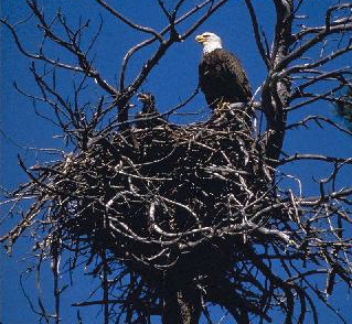
(g) Nest

(h) Diffusion

(i) Edge Aware Diffusion

(j) Egg

(k) Diffusion

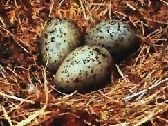
(l) Edge Aware Diffusion

Figure 4: Comparison between nonlinear anisotropic diffusion filtered results on input image (left column) using standard algorithm (middle column) and edge aware modified algorithm (right column). $\lambda=0.002$ and iterations=5 for all tests. For smoothing prior to taking derivatives, $\sigma_{S}=0.5$, and in the case of bilateral filter $\sigma_{R}=55$.

(a) $\lambda=0.0005,i=1$

(b) $\lambda=0.0005,i=2$

(c) $\lambda=0.0005,i=3$

(d) $\lambda=0.0005,i=4$

(e) $\lambda=0.0005,i=5$

(f) $\lambda=0.0105,i=1$

(g) $\lambda=0.0105,i=2$

(h) $\lambda=0.0105,i=3$

(i) $\lambda=0.0105,i=4$

(j) $\lambda=0.0105,i=5$

(k) $\lambda=0.0500,i=1$

(l) $\lambda=0.0500,i=2$

(m) $\lambda=0.0500,i=3$

(n) $\lambda=0.0500,i=4$

(o) $\lambda=0.0500,i=5$

Figure 5: Nonlinear anisotropic diffusion results on Challenge image using standard algorithm.

(a) $\lambda=0.0005,i=1$

(b) $\lambda=0.0005,i=2$

(c) $\lambda=0.0005,i=3$

(d) $\lambda=0.0005,i=4$

(e) $\lambda=0.0005,i=5$

(f) $\lambda=0.0105,i=1$

(g) $\lambda=0.0105,i=2$

(h) $\lambda=0.0105,i=3$

(i) $\lambda=0.0105,i=4$

(j) $\lambda=0.0105,i=5$

(k) $\lambda=0.0500,i=1$

(l) $\lambda=0.0500,i=2$

(m) $\lambda=0.0500,i=3$

(n) $\lambda=0.0500,i=4$

(o) $\lambda=0.0500,i=5$

Figure 6: Proposed edge aware nonlinear anisotropic diffusion results on Challenge image. $\sigma_{R}=55$ for the bilateral preconditioning in all cases.

7 Edge Aware Modifications for
the Bilateral Filter

Consider the 4-connected image graph where pixels are nodes and edges are weighted by the Euclidean distance between pixel colors. Then there exists a shortest path on the graph between any two pixels, and the length of this path is a representation of the combined spatial and range distance between the pixels which takes into account any discontinuities between them.

A traditional bilateral filter uses a spatial distance weight multiplied by a color dissimilarity weight. We propose to replace this bilateral weighting of range and distance treated separately by a single weighting of the shortest path distance on the image graph. This gracefully combines the two types of distances while properly accounting for edge awareness.

If the shortest path distance between pixels $p$ and $s$ is denoted by $d(p,s)$, then the modified bilateral filter can be written as

$$J_{s}=\frac{1}{k}\sum_{p\in\Omega}g(d(p,s))I_{p}$$ (7.1)

Writing the filter in this way suggests some other interesting filters, as well. For example, consider using the maximum edge distance instead of the sum of edge distances as the input to the Gaussian for weighting. Such a filter would eliminate gradients in the source image, while preserving solid colored regions, which might have interesting applications for image segmentation.

7.1 Performance Analysis of Edge Aware
Bilateral Filter

The time complexity of processing an image with the regular bilateral filter is $O(nd)$, where $n$ is the number of pixels and $d$ is the number of pixels defined in the (square) local neighborhood. Note that $d=4i^{2}$ in order to have a range of influence of $i$, so it is significantly more expensive than diffusion, which has complexity $O(ni)$ (for single processing architectures). In a massively parallel architecture, the bilateral filter could be done in $O(d)=O(i^{2})$ time and $O(1)$ communication, whereas diffusion would take $O(i)$ time and $O(i)$ communication.

Determining the path distance from a pixel $p$ to each neighbor $q\in N_{p}$ is an instance of the single-source shortest-paths problem [5]. It can be computed efficiently with Dijkstra’s algorithm [4] in $O(m\log n)$ time [5], for a graph with $n$ nodes and $m$ edges. Using the 4-connected image graph, each node contributes $\leq 2$ edges (eg, the edge above and to the left), so the total number of edges will be $\leq 2d$ (note that $|N_{p}|\approx d$). Thus, the time complexity for solving the single-source shortest-paths problem on a 4-connected image graph is $O(d\log d)$. Computing the bilateral weighted average would take $O(d)$ time already, so this is only an additional factor of $O(\log d)$.

Because of the special circumstances of this problem, some optimizations can be made such that the average case performance is significantly better than the worst case performance. First, it should be noted that the spatial range (which determines the size of $d$) is much less important, because there is no mathematical reason to induce an arbitrary cutoff on the range of influence. Rather, it is more intuitive to specify the range in terms of total path length.

If path length is used to specify the range of influence, then it is only necessary to compute the distance to pixels $q\in N_{p}$ if $d(p,q)<\tau_{R}$, where $\tau_{R}$ is a cutoff based on the range standard deviation $\sigma_{R}$. In these experiments, $\tau_{R}=3\sigma_{R}$. Because paths are found in increasing order using Dijkstra’s algorithm [4], this means that computation can terminate as soon as a path having length $>\tau_{R}$ is found.

In real images which do not usually contain large regions where each pixel has exactly the same intensity, there will only be a constant number of pixels that can be reached from $p$ without exceeding the maximum path cost $\tau_{R}$ regardless of spatial bandwidth. Therefore, the average case time complexity is $\lim_{d\to\infty}O(d\log d)=O(1)$. However, to protect the efficiency from suffering from a very high constant in homogeneous regions, a spatial cutoff should still be used in addition to $\tau_{R}$.

7.2 Experimental Results of Edge Aware Bilateral Filter

The original bilateral filter and the edge aware version are compared on a few test images in Fig. 7. A large spatial bandwidth is used specifically to highlight the limitations of the bilateral filter.

All of the images filtered with the standard bilateral filter exhibit a loss of saturation. In the Froud and Egg tests, this creates a somewhat surrealistic looking effect, because foreground colors are blended with background colors. In the Paris test, this is particularly noticeable in the flowers which acquire an orange hue. In the Eggs image, the color of the straw noticeably bleeds into the eggs. The bilateral filter does a fairly good job on the Nest image (due to the extremely simple histogram), but there is still some visible cloudy gray effects in the sky to the right and left of the nest (as well as desaturation of the sky).

In contrast, using the edge aware improved version based on shortest path distance, colors maintain their bright saturation in all of the tests in Fig. 7. Note that, in general, even better results could probably have been obtained by using a smaller bandwidth and more iterations (as is done in Fig. 9).

The algorithms are also compared on the Challenge image. In Fig. 8, the original bilateral filter is tested across a range of free parameter values. The free parameters are the usual $\sigma_{R}$ (standard deviation in the range dimension) and $\sigma$ (standard deviation in the spatial dimension). The effects of color cancellation are very prominent across all parameter ranges, and the noisy colored region is never satisfactory smoothed out.

The results using a range of parameters with the edge aware version is shown in Fig. 9. Note that these parameters are completely different from the free parameters of the original bilateral filter – $\sigma_{R}$ is the combined spatial-range parameter which is used on shortest path length. The spatial parameter is essentially irrelevant – we simply use a large value so that all path-lengths go to zero before reaching the boundary. However, we do introduce a new parameter $i$, number of iterations, which can be used to tweak the ‘spatial’ influence somewhat.

(a) Froud

(b) Bilateral

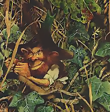
(c) Edge Aware Bilateral

(d) Paris

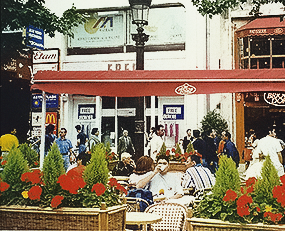
(e) Bilateral

(f) Edge Aware Bilateral

(g) Nest

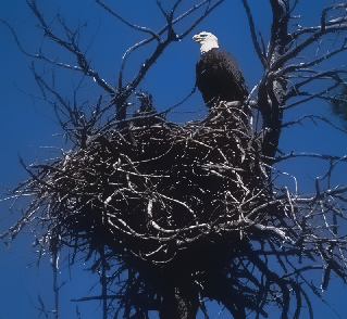
(h) Bilateral

(i) Edge Aware Bilateral

(j) Egg

(k) Bilateral

(l) Edge Aware Bilateral

Figure 7: Comparison between bilateral filtered results on input image (left column) using standard algorithm (middle column) and edge aware modified algorithm (right column). $\sigma_{S}=10$ and $\sigma_{R}=55$ for all tests ($\sigma_{R}$ is used as the combined spatial-range parameter in the edge aware version).

(a) $\sigma_{R}=20$,$\sigma=5$

(b) $\sigma_{R}=35$,$\sigma=5$

(c) $\sigma_{R}=50$,$\sigma=5$

(d) $\sigma_{R}=65$,$\sigma=5$

(e) $\sigma_{R}=80$,$\sigma=5$

(f) $\sigma_{R}=20$,$\sigma=10$

(g) $\sigma_{R}=35$,$\sigma=10$

(h) $\sigma_{R}=50$,$\sigma=10$

(i) $\sigma_{R}=65$,$\sigma=10$

(j) $\sigma_{R}=80$,$\sigma=10$

(k) $\sigma_{R}=20$,$\sigma=15$

(l) $\sigma_{R}=35$,$\sigma=15$

(m) $\sigma_{R}=50$,$\sigma=15$

(n) $\sigma_{R}=65$,$\sigma=15$

(o) $\sigma_{R}=80$,$\sigma=15$

Figure 8: Standard bilateral filtered results on Challenge image.

(a)

(b)

(c) $\sigma_{R}=50$,$i=1$

(d) $\sigma_{R}=65$,$i=1$

(e) $\sigma_{R}=80$,$i=1$

(f) $\sigma_{R}=20$,$i=2$

(g) $\sigma_{R}=35$,$i=2$

(h) $\sigma_{R}=50$,$i=2$

(i) $\sigma_{R}=65$,$i=2$

(j) $\sigma_{R}=80$,$i=2$

(k) $\sigma_{R}=20$,$i=3$

(l) $\sigma_{R}=35$,$i=3$

(m) $\sigma_{R}=50$,$i=3$

(n) $\sigma_{R}=65$,$i=3$

(o) $\sigma_{R}=80$,$i=3$

Figure 9: Proposed edge aware bilateral filtered results on Challenge, using $i$ filter iterations and combined spatial-range parameter $\sigma_{R}$.

8 Edge Aware Modifications
for Mean Shift

Because the mean shift filter also uses a bilateral weighted average, the computation of the mean shift vector can be done in an edge aware way by simply adopting the same modification that was proposed for the bilateral filter (5.2). However, we found that this additional computation does not improve the filtering result because the spatial bandwidth is typically small enough that multiple similarly colored distributions are not likely to occur within the support.

The more critical violation of edge awareness that that we wanted to fix occurs when a concave feature causes the mean to shift off of the feature. In order to fix this problem, we propose to compute the spatial component of the mean shift as normal, but to shift to a location that is a compromise between the mean shift vector and the image feature. There are many conceivable ways to accomplish this, and the method we use is by no means optimal, but it works well in all of our tests.

Specifically, we begin by defining the set $S$ to contain all pixels in the image with similar color to the current mean,

$$S=\left\{p\in\Omega:\frac{||I_{p}-s_{i}^{R}||}{h_{r}^{2}}<\tau\right\}$$ (8.1)

Then, if the next arithmetic spatial mean is $\mu$, we shift to the spatial point $\hat{p}$ defined by

$$\hat{p}=\operatorname*{argmin}_{p\in S}(p-\mu)^{2}$$ (8.2)

We found that using $\tau=0.5$ works well in general, and we use this value for all of our experiments.

8.1 Performance Analysis of Edge Aware Mean Shift

Finding the mode for each pixel requires $O(di)$ time, where $d$ is the number of pixels in the local neighborhood (determined by $h_{s}$) and $i$ is the number of iterations. Because the mean shift procedure is guaranteed to converge [3], $i$ is finite (for real images, the average number of iterations is almost always somewhere in the range of $[1.1,1.8]$ using the optimization mentioned below).

One of the optimizations proposed for the mean shift filter by Christoudias et. al [2] is to store the found mode for each pixel that falls on a mean shift path. Then, if another mean shift path falls upon a pixel that was previously on another path, the new mean shift path uses the previously found mode.

This makes the algorithm order-dependent and no longer guarantees that each pixel will be assigned to the correct mode of the kernel density estimate, but they found it to produce very good results about 5-6 times faster (although algorithmic time complexity is unchanged). This optimization is used in our implementation of mean shift as well.

8.2 Experimental Results of Edge Aware Mean Shift

A comparison of the filtered results is shown in Fig. 10. Figs. 11 and 12 show results on the Challenge image using the original and modified algorithms, respectively.

(a) Froud

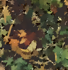
(b) Mean Shift

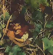
(c) Edge Aware Mean Shift

(d) Paris

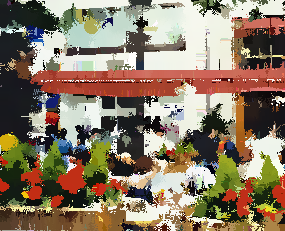
(e) Mean Shift

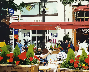
(f) Edge Aware Mean Shift

(g) Nest

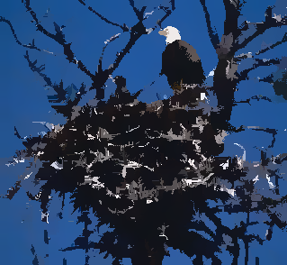
(h) Mean Shift

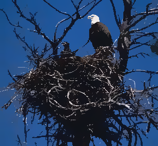
(i) Edge Aware Mean Shift

(j) Egg

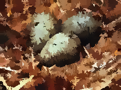
(k) Mean Shift

(l) Edge Aware Mean Shift

Figure 10: Comparison between mean shift filtered results on input image (left column) using standard algorithm (middle column) and edge aware modified algorithm (right column). $h_{s}=11$ and $h_{r}=55$ in all tests.

(a) $h_{s}=3$,$h_{r}=30$

(b) $h_{s}=5$,$h_{r}=30$

(c) $h_{s}=7$,$h_{r}=30$

(d) $h_{s}=9$,$h_{r}=30$

(e) $h_{s}=3$,$h_{r}=60$

(f) $h_{s}=5$,$h_{r}=60$

(g) $h_{s}=7$,$h_{r}=60$

(h) $h_{s}=9$,$h_{r}=60$

(i) $h_{s}=3$,$h_{r}=90$

(j) $h_{s}=5$,$h_{r}=90$

(k) $h_{s}=7$,$h_{r}=90$

(l) $h_{s}=9$,$h_{r}=90$

Figure 11: Standard mean shift filtered result on Challenge test image.

(a) $h_{s}=3$,$h_{r}=30$

(b) $h_{s}=5$,$h_{r}=30$

(c) $h_{s}=7$,$h_{r}=30$

(d) $h_{s}=9$,$h_{r}=30$

(e) $h_{s}=3$,$h_{r}=60$

(f) $h_{s}=5$,$h_{r}=60$

(g) $h_{s}=7$,$h_{r}=60$

(h) $h_{s}=9$,$h_{r}=60$

(i) $h_{s}=3$,$h_{r}=90$

(j) $h_{s}=5$,$h_{r}=90$

(k) $h_{s}=7$,$h_{r}=90$

(l) $h_{s}=9$,$h_{r}=90$

Figure 12: Proposed edge aware mean shift filtered result on Challenge test image.

The most notable difference between the original and edge aware modified filter results shown in Fig. 10 is that the edge aware version significantly cuts down on the ragged edges. A better looking filtered image could have been produced by using a smaller spatial bandwidth, but that changes the scale that is used to find modes in the kernel density estimate. The purpose of this test was to allow larger spatial bandwidths to be used to find large scale modes in homogeneous regions while still preserving fine detail in other regions. The modified filter accomplishes this.

In the Challenge test, the original algorithm creates many unsightly black artifacts (Fig. 11), and also causes some of the white pixels to get assigned into the red block at larger spatial bandwidths. The edge aware version preserves the strong black boundary lines while still clustering the underlying colors according to the kernel density estimate (Fig. 12).

As the scale grows larger, the edge aware version becomes progressively less “edge aware”, and eventually performs blurring across boundaries. A method for preventing this effect was mentioned in Section 8, but it was specifically not used because it disturbs the kernel density estimate too much.

9 Conclusions

Several successful approaches to the discontinuity preserving smoothing problem have been reviewed, illustrating an interesting conceptual dichotomy between viewing it as a global optimization problem vs. a class of algorithms related to diffusion. The global optimization approaches all minimize the same fundamental form using very different methods. Variable conductance diffusion is a direct application of physical diffusion, and anisotropic diffusion is a simple variant of variable conductance diffusion. The bilateral filter is a non-iterative approximation to diffusion, and we showed that the mean shift filter is an iterative generalization of the bilateral filter in higher dimensions.

We showed that edge awareness is a desirable property for unbiased discontinuity preserving smoothing for noise reduction, and demonstrated examples where each of the above algorithms violated the principle of edge awareness resulting in degraded image quality: the diffusion algorithm originally had problems maintaining edges after successive iterations, the bilateral filter had issues with color bleeding and loss of saturation (color cancellation), and the mean shift filter created significant artifacts for non-convex colored regions when using large spatial bandwidths.

Finally, we proposed individual modifications to each algorithm to account for edge awareness and showed how these modifications could be implemented with little or no change in algorithm complexity. After making the changes, visual improvements were easily visible in the smoothed results.

References

- [1] R. T. Chin, C. L. Yeh, “Quantitative evaluation of some edgepreserving noise-smoothing techniques,” CVGIP, 23:67 91, 1983.
- [2] C. M. Christoudias, B. Georgescu, P. Meer, “Synergism in low level vision,” 16th Intl. Conf. on Pattern Recognition, Vol. 4, pp.150-155, 2002.
- [3] D. Comaniciu, P. Meer, “Mean Shift: A Robust Approach Towards Feature Space Analysis,” IEEE Trans. on Pattern Analysis and Machine Int., Vol. 24, No. 5, 2002.
- [4] E. W. Dijkstra, “A Note on two problems in connection with graphs,” Numerische Matematik, Vol. 1, pp.269-271, 1959.
- [5] J. Kleinberg and E. Tardos, Algorithm Design. San Francisco, CA: Addison-Wesley, 2006.
- [6] G. Sapiro, D. Ringach, “Anisotropic diffusion of color images,” Proc. SPIE, Vol. 2657, 1996.
- [7] W. Snyder and H. Qi, Machine Vision. Cambridge, England: Cambridge University Press, 2004.
- [8] C. Tomasi, R. Manduchi, “Bilateral Filtering for Gray and Color Images,” Proc. of the 1998 IEEE Intl. Conf. on Computer Vision, pp. 839-846.
- [9] Y. Han, W. Snyder, G. Bilbro, “Discontinuity Preserving Smoothing of Multivariate MR Images Using Vector Mean Field Annealing,” J. of Mathematical Imaging and Vision, Vol. 9, pp.199-212, 1998.
- [10] D. Scharstein and R. Szeliski, “A taxonomy and evaluation of dense two-frame stereo correspondence algorithms,” Int. Journal of Computer Vision, Vol. 47, pp.7-42, 2002.
- [11] M. Black, A. Rangarajan, “The Outlier Process: Unifying Line Processes and Robust Statistics,” IEEE Conf. on Comp. Vision and Pattern Recognition (CVPR 94), Seattle, WA, June 1994.
- [12] A. Blake, A. Zisserman, Visual Reconstruction., The MIT Press, Cambridge, Massachusetts, 1987.
- [13] P. F. Felzenszwalb, D. P. Huttenlocher, “Efficient Belief Propagation for Early Vision,”Int. Journal of Computer Vision, Vol. 70, No. 1, 2006.
- [14] Y. Boykov, O. Veksler, R. Zabih, “Fast approximate energy minimization via graph cuts,” Pattern Analysis and Machine Intelligence, Vol. 23, Issue 11, pp.1222 - 1239, Nov 2001.
- [15] Y. Boykov, V. Kolmogorov, “An Experimental Comparison of Min-Cut/Max-Flow Algorithms for Energy Minimization in Vision,” IEEE Trans. on PAMI, Vol. 26, No. 9, pp. 1124-1137, 2004.
- [16] D. Greig, B. Porteous, A. Seheult, “Exact maximum a posteriori estimation for binary images,” Journal of the Royal Statistical Society, Series B, Vol. 51, Issue 2, pp.271 279, 1989.
- [17] S. Grossberg, “Neural Dynamics of Brightness Perception: Features, Boundaries, Diffusion, and Resonance,” Perceptino and Psychophysics, 36(5), pp.428-456, 1984.
- [18] N. Nordstrom, “Biased Anisotropic Diffusion – A Unified Regularization and Diffusion Approach to Edge Detection,” Image and Vision Computing, 8(4), pp.318-327, 1990.
- [19] P. Perona, J. Malik, “Scale-Space and Edge Detection using Anisotropic Diffusion,” IEEE Trans. on Patt. Analysis and M. Int (PAMI), 16(4), 1994.
- [20] D. Barash, “Bilateral Filtering and Anisotropic Diffusion: Towards a Unified Viewpoint”, In Third International Conference on ScaleSpace and Morphology, pp.273-280, 2000.
- [21] E. Wasserstrom, “Numerical solutions by the continuition method,” SIAM Review, 15:89–119, 1973.
- [22] J. Zerubia, R. Chellappa, “Mean Field Annealing Using Compound Gauss-Markov Random Fields for Edge Detection and Image Estimation,” IEEE Trans. on Neural Networks, 4(4), 1993.